Dynamical Monte Carlo investigation of spin reversals and nonequilibrium magnetization of single-molecule magnets

Abstract

In this paper, we combine thermal effects with Landau-Zener (LZ) quantum tunneling effects in a dynamical Monte Carlo (DMC) framework to produce satisfactory magnetization curves of single-molecule magnet (SMM) systems. We use the giant spin approximation for SMM spins and consider regular lattices of SMMs with magnetic dipolar interactions (MDI). We calculate spin reversal probabilities from thermal-activated barrier hurdling, direct LZ tunneling, and thermal-assisted LZ tunnelings in the presence of sweeping magnetic fields. We do systematical DMC simulations for Mn₁₂ systems with various temperatures and sweeping rates. Our simulations produce clear step structures in low-temperature magnetization curves, and our results show that the thermally activated barrier hurdling becomes dominating at high temperature near 3K and the thermal-assisted tunnelings play important roles at intermediate temperature. These are consistent with corresponding experimental results on good Mn₁₂ samples (with less disorders) in the presence of little misalignments between the easy axis and applied magnetic fields, and therefore our magnetization curves are satisfactory. Furthermore, our DMC results show that the MDI, with the thermal effects, have important effects on the LZ tunneling processes, but both the MDI and the LZ tunneling give place to the thermal-activated barrier hurdling effect in determining the magnetization curves when the temperature is near 3K. This DMC approach can be applicable to other SMM systems, and could be used to study other properties of SMM systems.

I Introduction

Single-molecule magnet (SMM) systems attract more and more attention because they can be used to make devices for spintronic applications spintr1 ; spintr2 , quantum computing qc , high-density magnetic information storage mem etc ad21 ; bb ; ad22 . Usually, a SMM can be treated as a large spin with strong magnetic anisotropy at low temperature. The most famous and typical is Mn₁₂-ac ([Mn₁₂O₁₂(Ac)₁₆(H₂O)₄]$\cdot$2HAc$\cdot$4H₂O, where HAc=accetic acid), or Mn₁₂ for short Mn12a . It usually has spin $S=10$ and large anisotropy energy, producing a high spin reversal barrier sessoli . Many interesting phenomena have been observed, such as various dynamical magnetism. One of the most intriguing phenomena observed in SMM systems is a step-wise structure in low-temperature magnetization curves mstep1 ; mstep2 ; mstep3 . Great efforts have been made to investigate this phenomenon and related effects add1 ; chio ; Mn12tBuAc ; TB ; Mn4b ; book ; Mn12para1 ; Mn12E . The step-wise structure is attributed to Landau-Zener (LZ) quantum tunneling effect Landau ; Zener . This stimulates intensive study on LZ model and its variants lz1 ; lz2 ; lz3 ; lzepl ; lz4 ; lz5 ; lz6 ; lz7 ; lz8 . Some authors use numeric diagonalization methods numeric1 ; numeric2 to study many-level LZ models to understand the step structure in experimental magnetization curves. However, it is difficult to consider thermal effects in these approaches to obtain satisfactory magnetization curves comparable to experimental results.

In this paper, we shall combine the classical thermal effects with the quantum LZ tunneling effects in a dynamical Monte Carlo (DMC) framework dmc0 ; dmc1 ; gbliu in order to produce satisfactory magnetization curves comparable to experimental results. We consider ideal tetragonal body-centered lattices and use the giant spin approximation for spins of SMMs. We consider magnetic dipolar interactions, but neglect other factors such as defects, disorders, and misalignments between the easy axis and applied magnetic field. We calculate spin reversal probabilities from thermal-activated barrier hurdling, direct LZ tunneling effect, and thermal-assisted LZ tunneling effects in the presence of sweeping magnetic fields, and thereby derive a unified probability expression for any temperature and any sweeping field. Taking the Mn₁₂ as example, we do systematical DMC simulations with various temperatures and sweeping rates. The step structure appears in our simulated low-temperature magnetization curves, and our simulated magnetization curves are semi-quantitatively consistent with corresponding experimental results on those good Mn₁₂ systems (with less disorders) in the presence of little misalignments between the easy axis and applied fields Mn12tBuAc ; TB . Interplays of the LZ tunneling effect, the thermal effects, and the magnetic dipolar interactions are elucidated. These imply that our simple model and DMC method capture the main features of experimental magnetization curves for little misalignments. More detailed results will be presented in the following.

The rest of this paper is organized as follows. In next section we shall define our spin model and describe approximation strategy. In the third section we shall describe our simulation method, present our unified probability formula for the spin reversal from the three spin reversal mechanisms, and give our simulation parameters. In the fourth section we shall present our simulated magnetization curves and some analysis. In the fifth section we shall show the key roles of the dipolar interactions in determining LZ tunneling probabilities. Finally, we shall give our conclusion in the sixth section.

II Spin Model and approximation

Without losing generality, we take typical Mn₁₂ system as our sample in the following. Under giant spin approximation, every Mn₁₂ SMM is represented by a spin $S$=10. Magnetic dipolar interactions are the only inter-SMM interactions, with hyperfine interactions neglected. Mn₁₂ SMMs are arranged to form a body-centered tetragonal lattice with experimental lattice parametersMn12abc . Using a body-centered tetragonal unit cell that consists of two SMMs, we define our lattice as $L_{1}\times L_{2}\times L_{3}$, where $L_{1}$, $L_{2}$, and $L_{3}$ are three positive integers. A longitudinal magnetic field $B_{z}(t)=B_{0}+\nu t$ is applied along the $c$-easy axis of magnetization, where $\nu$ is the field-sweeping rate and $B_{0}$ is the starting magnetic field. The total Hamiltonian of this system can be expressed as

$$\hat{H}=\sum_{i}\hat{H}_{i}^{0}+\frac{1}{2}\sum_{i\neq j}\hat{H}_{ij}^{\rm di}~{},$$ (1)

where $\hat{H}_{i}^{0}$ is the single-body part for the $i$-th single SMM, and $\hat{H}_{ij}^{\rm di}$ describes the magnetic dipolar interaction between the $i$-th and $j$-th SMM. The factor $1/2$ before the sum sign is due to the double counting in the summation. $\hat{H}_{i}^{0}$ is given by

$$\hat{H}_{i}^{0}= -D(\hat{S}_{i}^{z})^{2}+E[(\hat{S}_{i}^{x})^{2}-(\hat{S}_{i}^{y})^{2}]$$ (2)

$$+B_{4}^{0}\hat{O}_{4}^{0}+B_{4}^{4}\hat{O}_{4}^{4}+g\mu_{B}B_{z}\hat{S}_{i}^{z}~{},$$

where $\hat{\mathbf{S}}_{i}\equiv(\hat{S}_{i}^{x},\hat{S}_{i}^{y},\hat{S}_{i}^{z})$ is the spin vector operator for the $i$-th SMM, $g$ the Landé g-factor (here $g=2$ is used), $\mu_{B}$ the Bohr magneton, $D$, $E$, $B_{4}^{0}$ and $B_{4}^{4}$ are all anisotropic parameters, and $\hat{O}_{4}^{0}$ and $\hat{O}_{4}^{4}$ are both Steven operatorsbook defined by $\hat{O}_{4}^{0}=35(\hat{S}_{i}^{z})^{4}-[30S(S+1)-25](\hat{S}_{i}^{z})^{2}+3S^{2}(S+1)^{2}-6S(S+1)$ and $\hat{O}_{4}^{4}=[(\hat{S}_{i}^{+})^{4}+(\hat{S}_{i}^{-})^{4}]/2$. $\hat{H}_{ij}^{\rm di}$ is defined by

$$\hat{H}_{ij}^{\rm di}=\frac{\mu_{0}g^{2}\mu^{2}_{B}}{4\pi r^{3}_{ij}}[\hat{\mathbf{S}}_{i}\cdot\hat{\mathbf{S}}_{j}-\frac{3}{r^{2}_{ij}}(\hat{\mathbf{S}}_{i}\cdot\mathbf{r}_{ij})(\hat{\mathbf{S}}_{j}\cdot\mathbf{r}_{ij})]~{},$$ (3)

where $\mu_{0}$ is the magnetic permeability of vacuum, and $\mathbf{r}_{ij}$ the vector from $i$ to $j$, with $r_{ij}$=$|\mathbf{r}_{ij}|$ being the distance between $i$ and $j$.

For the $i$-th SMM, we treat all the effects from the other SMMs by classical-spin approximation. As a result, we derive the partial Hamiltonian $\hat{H}_{i}$ that acts on the $i$-th SMM:

$$\!\hat{H}_{i} \!\!=\!\! \hat{H}_{i}^{0}+g\mu_{B}\mathbf{B}_{i}^{\rm di}\cdot\hat{\mathbf{S}}_{i}$$ (4)

$$\!\!=\!\! -D(\hat{S}_{i}^{z})^{2}+B_{4}^{0}\hat{O}_{4}^{0}+\hat{H}_{i}^{\rm tr}+g\mu_{B}(B_{z}+B_{iz}^{\rm di})\hat{S}_{i}^{z},$$

where the transverse part $\hat{H}_{i}^{\rm tr}$ is defined as

$$\hat{H}_{i}^{\rm tr}=E[(\hat{S}_{i}^{x})^{2}\!-\!(\hat{S}_{i}^{y})^{2}]+B_{4}^{4}\hat{O}_{4}^{4}+g\mu_{B}(B_{ix}^{\rm di}\hat{S}_{i}^{x}\!+\!B_{iy}^{\rm di}\hat{S}_{i}^{y}).$$ (5)

For the $i$-th SMM, the dipolar interaction of the other SMMs is equivalent to $\mathbf{B}_{i}^{\rm di}\equiv(B_{ix}^{\rm di},B_{iy}^{\rm di},B_{iz}^{\rm di})=\sum_{j(\neq i)}\mathbf{B}_{ji}$, where $\mathbf{B}_{ji}$ is the magnetic dipolar field applied by the $j$-th SMM on the $i$-th SMM. It contributes a magnetic field consisting of longitudinal and transverse parts.

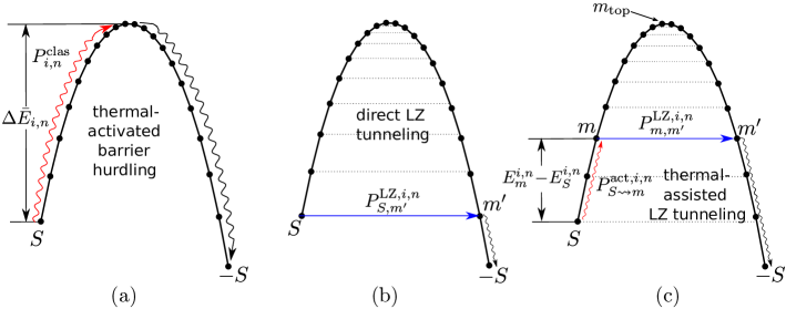
Figure 1: (Color online.) A schematic demonstration of the three spin reversal mechanisms: (a) thermal-activated barrier hurdling, (b) direct LZ tunneling, and (c) thermal-assisted LZ tunneling. The probabilities, energy levels, barrier, and other symbols are defined in the text. The horizontal solid line with arrow in (b) and (c) shows that a pair of energy levels satisfy the resonance tunneling conditions. The horizontal dotted lines in (b) and (c), as guide for eyes, imply that these energy levels do not match.

III Simulation method and parameters

As we show in Fig. 1, there are three main mechanisms related to the reversal of a SMM spin sessoli ; book ; mstep1 ; mstep2 ; mstep3 ; add1 ; lz1 ; lzepl : (a) thermal-activated barrier-hurdling, (b) direct LZ tunneling, and (c) thermal-assisted LZ tunneling. The thermal-activated barrier hurdling dominates at high temperature (if the blocking temperature $T_{B}\sim$3.3K for Mn₁₂ TB is treated as high temperature), the direct LZ tunneling at low temperature, and the thermal-assisted LZ tunneling at intermediate temperature. For any temperature, we consider all the three spin reversal mechanisms simultaneously. For the time scale we are interested, we do not need to treat phonon-related interactions directly, but shall use an effective transition-state theory to calculate the thermal-activated spin-reversal rates. We shall use a DMC method to combine the quantum LZ tunneling effects with the classical thermal effects. Various kinetic Monte Carlo (KMC) methodswitten ; kmc1 ; kmc2 ; lbg99 ; kmc3 , essentially similar to this DMC method, have been used to simulate atomic kinetics during epitaxial growth for many years. On the other hand, MC simulation has been used to study Glauber dynamics of kinetic Ising modelsglauber ; ad23 ; ad24 . We shall present a detailed description of this DMC simulation method in the following.

III.1 Thermal-activated spin reversal probability

We need the thermal-activated energy barrier in order to calculate the thermal-activated spin-reversal rate. When calculating the thermal-activated energy barrier we ignore the small transverse part $\hat{H}_{i}^{\rm tr}$ and use classical approximation for the spin operators. The large spin $S=10$ of Mn₁₂ further supports the approximations. As a result, the energy of the $i$-th SMM can be expressed as

$$\bar{E}_{i}=-D_{2}(S_{i}^{z})^{2}-D_{4}(S_{i}^{z})^{4}+h_{i}S_{i}^{z}~{},$$ (6)

where $S_{i}^{z}$ is the classical variable for the spin operator $\hat{S}_{i}^{z}$, $h_{i}=g\mu_{B}(B_{z}+B_{iz}^{\rm di})$, $D_{2}=D+[30S(S+1)-25]B_{4}^{0}$, and $D_{4}=-35B_{4}^{0}$. Because $h_{i}$ is dependent on time $t$, $\bar{E}_{i}$ changes with $t$.

We define our MC steps by the time points, $t_{n}=\Delta t\cdot n$, where $n$ takes nonnegative integers in sequence. For the $n$-th MC step, we use $\bar{E}_{i,n}$, $h_{i,n}$, and $S_{i,n}^{z}$ to replace $\bar{E}_{i}$, $h_{i}$, and $S_{i}^{z}$. Because each of the spins has two equilibrium orientations along the easy axis, we assume every spin takes either $S$ or $-S$ at each of the times $t_{n}$. Within the $n$-th MC step ($t$: from $t_{n}$ to $t_{n+1}$), we use an angle variable $\theta_{i,n}$ to describe the $i$-th spin’s deviation from its original ($t_{n}$) orientation $S_{i,n}^{\rm eq}$. Naturally, $\theta_{i,n}=0$ corresponds to the original state and $\theta_{i,n}=\pi$ is the reversed state, and then all the other angle values ($0<\theta_{i,n}<\pi$) are treated as transition states. Expressing $S_{i,n}^{z}$ as $S_{i,n}^{\rm eq}\cos\theta_{i,n}$, we usually have a maximum in the curve of $\bar{E}_{i,n}(\cos\theta_{i,n})$ as a function of $\cos\theta_{i,n}$, and the maximum determines the energy barrier for the spin reversal mechanismliying1 ; liying2 ; lbg , as shown in Fig. 1(a). We define $x_{i,n}=\cos\theta_{i,n}$ for convenience. We have $-1\leq x_{i,n}\leq 1$ for actual $\theta_{i,n}$, but $x_{i,n}$ can be extended beyond this region in order to always obtain a formal solution $x_{i,n}^{\rm max}$ for the maximum. $|x_{i,n}^{\rm max}|<1$ implies that there actually exists an energy barrier, and $|x_{i,n}^{\rm max}|\geq 1$ means that there is no barrier for the corresponding process. Under conditions $D_{2}>0$ and $D_{4}>0$, the barrier can be expressed as:

$$\Delta\bar{E}_{i,n}=\left\{\begin{array}[]{lll}\bar{E}_{i,n}(x_{i,n}^{\rm max}),&&|x_{i,n}^{\rm max}|\leq 1\\ \bar{E}_{i,n}(-1)=|2h_{i,n}S_{i,n}^{\rm eq}|,&&x_{i,n}^{\rm max}<-1\\ \bar{E}_{i,n}(1)=0,&&x_{i,n}^{\rm max}>1\end{array}\right.$$ (7)

where $x_{i,n}^{\rm max}$ is defined by

$$x_{i,n}^{\rm max}=\sqrt[3]{-q_{i,n}/2+\sqrt{d_{i,n}}}+\sqrt[3]{-q_{i,n}/2-\sqrt{d_{i,n}}}$$ (8)

and the three parameters are defined by $d_{i,n}=(q_{i,n}/2)^{2}+(p/3)^{3}$, $p=D_{2}/(2D_{4}S^{2})$, and $q_{i,n}=-h_{i,n}S_{i,n}^{\rm eq}/(4D_{4}S^{4})$. These parameters are dependent on the spin configuration and the magnetic field, and then on the time $t_{n}$ (or $n$).

The spin reversal rate within the $n$-th MC step (between $t_{n}$ and $t_{n+1}$) can be expressed as $R_{i,n}=R_{0}\exp(-\Delta\bar{E}_{i,n}/k_{B}T)$ in terms of Arrhenius law ArrheniusLaw2 , where $k_{B}$ is the Boltzmann constant and $R_{0}$ the characteristic attempt frequency. We use $P_{n}(t^{\prime})$ to describe the probability that the $i$-th spin is reversed between $0$ and $t^{\prime}$, where $t^{\prime}$ satisfies the condition $t^{\prime}\leq\Delta t$. It has the initial condition $P_{n}(t^{\prime}=0)=0$ and satisfies the equation $[1-P_{n}(t^{\prime})]\cdot R_{n}(t^{\prime})dt^{\prime}=P_{n}(t^{\prime}+dt^{\prime})-P_{n}(t^{\prime})$, or

$$[1-P_{n}(t^{\prime})]R_{n}(t^{\prime})=\frac{d}{dt^{\prime}}P_{n}(t^{\prime})$$ (9)

where $R_{n}(t^{\prime})$, the reversal rate at $t^{\prime}$, is taken as the rate $R_{i,n}$, independent of $t^{\prime}$ within the region [0,$\Delta t$]. Solving the equation, we obtain the probability $P^{\rm clas}_{i,n}$ defined as $P_{n}(t^{\prime}=\Delta t)$ for a classical thermal-activated reversal of the $i$-th spin within the $n$-th MC step:

$$P^{\rm clas}_{i,n}=1-\exp(-\Delta t\cdot R_{i,n}).$$ (10)

For $\Delta t\ll 1/R_{i,n}$, Eq. (10) reduces to $P^{\rm clas}_{i,n}=\Delta t\cdot R_{i,n}$. The probability expression defined in Eq. (10) is reasonable because $P^{\rm clas}_{i,n}$ will not exceed unity even when $\Delta t$ is very large with respect to $1/R_{i,n}$.

III.2 LZ-tunneling related spin reversal probabilities

When temperature is lower than $T_{B}$, LZ tunneling begins to contribute to spin reversal. We begin with the effective quantum single-spin Hamiltonian (4) with (5). All the effects of other spins are included in the magnetic dipolar field $\mathbf{B}_{i}^{\rm di}$ (depending on the time $t$) and are depending on the magnetic field and the current spin configuration. For the $n$-th MC step, if the transverse term $\hat{H}_{i}^{\rm tr}$ is removed, Hamiltonian Eq. (4) is diagonal and has $2S+1$ energy levels, $E_{m}^{i,n}$, where $m$ can take any of $S,S-1,\cdots,-(S-1),-S$. If using the continuous time variable $t$, we can express the energy levels as $E_{m}^{i}(t)$ (with $m$ from $S$ to -$S$) and derive their crossing fields [at which $E_{m}^{i}(t)=E_{m^{\prime}}^{i}(t)$]:

$$B_{m,m^{\prime}}=\frac{(m+m^{\prime})[D_{2}+D_{4}(m^{2}+m^{\prime 2})]}{g\mu_{B}}.$$ (11)

The transverse term $\hat{H}_{i}^{\rm tr}$ will modify the energy levels $E_{m}^{i,n}$, but the $2S+1$ energy levels of Hamiltonian (4) with (5), $\tilde{E}_{m}^{i,n}$, can be still labelled by $m=S,S-1,\cdots,-(S-1),-S$. Actually, the difference between $E_{m}^{i,n}$ and $\tilde{E}_{m}^{i,n}$ is small. Due to the existence of the transverse part $\hat{H}_{i}^{\rm tr}$, there will be an avoided level crossing between $\tilde{E}_{m}^{i,n}$ and $\tilde{E}_{m^{\prime}}^{i,n}$ for the $n$-th MC step when the effective field $B_{z}+B_{iz}^{\rm di}$ equals $B^{i,n}_{m,m^{\prime}}$, with $m$ and $m^{\prime}$ taking values among $S,S-1,\cdots,-(S-1),-S$. The set of all the $B^{i,n}_{m,m^{\prime}}$ values are the effective field conditions for the avoided-level-crossings. If $E_{m}^{i,n}$ equals $E_{m^{\prime}}^{i,n}$, $B^{i,n}_{m,m^{\prime}}$ is approximately equivalent to the crossing field (equaling $B_{m,m^{\prime}}$). The allowed $(m,m^{\prime})$ pairs are shown in Fig. 2. This means that when $B_{z}$ is swept to a right $B_{m,m^{\prime}}^{i,n}-B_{iz}^{\rm di}$ value, a quantum tunneling occurs between the $m$ and $m^{\prime}$ states. The tunneling can be well described using LZ tunnelinggbliu ; Mn4b ; numeric1 ; numeric2 . The nonadiabatic LZ tunneling probability $P^{{\rm LZ},i,n}_{m,m^{\prime}}$ is given byLandau ; Zener

$$P^{{\rm LZ},i,n}_{m,m^{\prime}}=1-\exp\Bigg{[}-\frac{\pi(\Delta_{m,m^{\prime}}^{i,n})^{2}}{2\hbar g\mu_{B}|m-m^{\prime}|\nu}\Bigg{]}~{},$$ (12)

where the tunnel splitting $\Delta^{i,n}_{m,m^{\prime}}$ is the energy gap at the avoided crossing of states $m$ and $m^{\prime}$. $B^{i,n}_{m,m^{\prime}}$ and $\Delta^{i,n}_{m,m^{\prime}}$ can be calculated by diagonalizing Eq. (4). If the dipolar field is neglected, $B^{i,n}_{m,m^{\prime}}$, $\Delta^{i,n}_{m,m^{\prime}}$, and $P^{{\rm LZ},i,n}_{m,m^{\prime}}$ reduce to $B^{0}_{m,m^{\prime}}$, $\Delta^{0}_{m,m^{\prime}}$, and $P^{0}_{m,m^{\prime}}$, those of corresponding isolated SMMs, respectively.

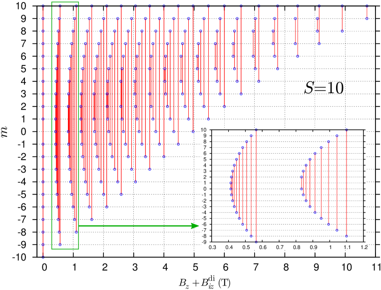
Figure 2: (Color online.) A schematic demonstration for the conditions of the $i$-th spin that Landau-Zener tunnelings can happen. $m$ labels the spin $z$ component, from -10 to 10, and $B_{z}+B_{iz}^{\rm di}$ is the effective magnetic field. A hollow circle indicates one of the allowed $m$ values. The two circles ($m$ and $m^{\prime}$) connected with one vertical line means that a LZ tunneling condition is satisfied between the two states at the corresponding effective field $B^{i,n}_{m,m^{\prime}}$ within the $n$-th MC step. There is at most one LZ tunneling at any nonzero value of the effective field, but every $m$ state can tunnel to the -$m$ state when the effective field is zero. The inset amplifies the part between 0.3 and 1.2 T.

At the beginning of field sweeping, we let all the spins have $m=S$. If $T\!\ll\!T_{B}$, thermal activations are frozen, and LZ tunnelings only occur at the avoided crossings $(S,m^{\prime})$, where $m^{\prime}$ takes one of $-S,-S+1,\cdots,S-1$. This is the direct tunneling shown in Fig. 1(b), and the LZ tunneling probability is given by

$$P^{\rm dLZ}_{i,n}=P_{S,m^{\prime}}^{{\rm dir},i,n}=P_{S,m^{\prime}}^{{\rm LZ},i,n}.$$ (13)

It is nonzero only when the condition $E_{S}^{i,n}=E_{m^{\prime}}^{i,n}$ is satisfied. When the temperature is in the intermediate region $0\ll T<T_{B}$, the thermal-assisted tunneling plays an important role. This process can be represented by $S\rightsquigarrow m\rightarrow m^{\prime}$ as shown in Fig. 1(c), in which $S$ and $m$ states lie on one side of the thermal barrier and $m^{\prime}$ and $-S$ states on the other side. The first process $S\rightsquigarrow m$ means that a spin is thermally activated from $S$ to $m$ state with the probability $P_{S\rightsquigarrow m}^{\text{act},i,n}$, which is given by $P_{S\rightsquigarrow m}^{\text{act},i,n}=1-\exp(-\Delta t\cdot R^{\text{act}}_{i,n})$, where $R^{\text{act}}_{i,n}$ is given by $R_{0}\exp[-(E_{m}^{i,n}-E_{S}^{i,n})/k_{B}T]$. The second process $m\rightarrow m^{\prime}$ is the LZ tunneling from $m$ to $m^{\prime}$, with the probability defined in Eq. (12). Therefore, the reversal probability of thermal-assisted LZ tunneling through $m$ is given by

$$P^{\rm taLZ}_{i,n,m}=P_{S\rightsquigarrow m\rightarrow m^{\prime}}^{\text{ass},i,n}=P_{S\rightsquigarrow m}^{\text{act},i,n}P_{m,m^{\prime}}^{{\rm LZ},i,n}.$$ (14)

It is nonzero only when the condition $E_{m}^{i,n}=E_{m^{\prime}}^{i,n}$ is satisfied.

It must be pointed out that $m^{\prime}$ in $P_{S,m^{\prime}}^{{\rm dir},i,n}$ and $P_{S\rightsquigarrow m\rightarrow m^{\prime}}^{\text{ass},i,n}$ is determined by $E_{m^{\prime}}^{i,n}=E_{S}^{i,n}$ and $E_{m^{\prime}}^{i,n}=E_{m}^{i,n}$, respectively, as is shown in Figs. 1(b) and 1(c). If the energy-level condition is satisfied, the probability is larger than zero; or else the probability is equivalent to zero. Therefore, the subscript $m^{\prime}$ in $P_{S,m^{\prime}}^{{\rm dir},i,n}$ and $P_{S\rightsquigarrow m\rightarrow m^{\prime}}^{\text{ass},i,n}$ can be removed, as we have done in $P^{\rm dLZ}_{i,n}$ and $P^{\rm taLZ}_{i,n,m}$.

III.3 Unified spin reversal probability for MC simulation

Generally speaking, every one of the three spin reversal mechanisms takes action at any given temperature. Actually the LZ tunneling effect dominates at low temperatures and the thermal effects become more important at higher temperatures. For the $n$-th MC step, the probability for the thermal-activated barrier-hurdling reversal of the $i$-th spin is given by $P^{\rm clas}_{i,n}$ defined in Eq. (10) [see Fig. 1(a)], that for the direct LZ tunneling effect equals $P^{\rm dLZ}_{i,n}$ defined in Eq. (13) [see Fig. 1(b)], and that for the thermal-assisted LZ tunneling effects through the $m$ state is given by $P^{\rm taLZ}_{i,n,m}$ defined in Eq. (14) [see Fig. 1(c)]. Here the partial probabilities from the three mechanisms are considered independent of each other. Therefore, we can derive the total probability $P_{i,n}^{\rm tot}$ for the reversal of the $i$-th spin within the $n$-th MC step:

$$P_{i,n}^{\rm tot}=1-(1-P_{i,n}^{\rm clas})(1-P^{\rm dLZ}_{i,n})\!\!\prod_{m_{\rm top}<m<S}\!\!(1-P^{\rm taLZ}_{i,n,m}),$$ (15)

where $m_{\rm top}$, depending on the effective field, is determined by the highest level $E^{i,n}_{m_{\rm top}}$ among the $2S$ energy levels, $E^{i,n}_{m}$ ($-S\leq m<S$), as we show in Fig. 1(c).

It must be pointed out that $P_{i,n}^{\rm clas}$ is always larger than zero, but the LZ-tunneling related probabilities, $P^{\rm dLZ}_{i,n}$ and $P^{\rm taLZ}_{i,n,m}$, are nonzero only at some special values of the effective field. As is shown in Fig. 2, there is at most one LZ-tunneling channel, from either direct or thermal-assisted LZ effect, for a given nonzero value of the effective field. As a result, when the effective field is nonzero, we have at most one nonzero value from either $P^{\rm dLZ}_{i,n}$ or one of $P^{\rm taLZ}_{i,n,m}$ ($m_{\rm top}<m<S$). It is only at the zero value of the effective field that both $P^{\rm dLZ}_{i,n}$ and $P^{\rm taLZ}_{i,n,m}$ ($0<m<S$) ($m_{\rm top}=0$) can be larger than zero so that we can have the direct LZ tunneling and all the thermal-assisted LZ-tunneling channels simultaneously. In our simulations, the processes that a reversed spin is reversed again are also considered, but the probabilities are tiny.

III.4 Simulation parameters

We use experimental lattice constants, $a=b=17.1668\,\text{\AA}$ and $c=12.2545\,\text{\AA}$, and experimental anisotropy parameters, $D/k_{B}=0.66$ K, $B_{4}^{0}/k_{B}=-3.2\times 10^{-5}$ K, and $B_{4}^{4}/k_{B}=6\times 10^{-5}$ K Mn12abc ; Mn12tBuAc ; Mn12para1 . As for the second-order transverse parameter $E$, $E/k_{B}=1.8\times 10^{-3}$ K is taken from the average of experimental values Mn12E . We describe the time by using both continuous variable $t$ and discrete superscript/subscript $n$. In some cases, the sweeping field can be used to describe the time because it is defined by $B_{z}(t)=B_{0}+\nu t$. There is always a nonnegative integer $n$ for any given $t$ value, and there is a $t$ region, [$t_{n},t_{n+1}$], for any given nonnegative $n$. We take $\Delta t=0.1$ ms and $R_{0}=10^{9}$/s, which guarantee the good balance between computational demand and precision.

The dipolar fields $(B_{ix}^{\rm di},B_{iy}^{\rm di},B_{iz}^{\rm di})$ at each SMM are updated whenever any of the SMM spins is reversed. The $\Delta^{i,n}_{m,m^{\prime}}$ values are recalculated whenever any LZ tunneling happens. In the simulations, the field $B_{z}$ is swept from -7 to 7 T in the forward process, and the full magnetization hysteresis loop is obtained simply by using the loop symmetry. Every magnetization curve is calculated by averaging over 100 runs to make statistical errors small enough. The main results presented in the following are simulated and calculated with lattices consisting approximately of $900\sim 1200$ body-centered unit cells or $1800\sim 2400$ spins. We have test our results with lattices consisting approximately of 100 $\sim$ 6000 body-centered unit cells, or 200 $\sim$ 12000 spins.

IV simulated magnetization curves

Presented in Fig. 3 are simulated magnetization curves (with $M$ normalized to the saturated value $M_{S}$) against the applied sweeping field $B_{z}$ for ten different temperatures: 0.1, 0.5, 0.6, 0.8, 1.0, 1.5, 2.0, 2.5, 2.8, and 3.2 K. Here, the lattice dimension is $10\times 10\times 10$ and the field sweeping rate is 0.02 T/s. Each of the curves is calculated by averaging over 100 runs. The curves of 0.1 K and 0.5 K fall in the same curve, which implies that thermal activation is totally frozen when the temperature is below 0.5 K. It can be seen in Fig. 3 that the area enclosed by a magnetization loop decreases with the temperature increasing, becoming nearly zero at 3.2 K (near the blocking temperature 3.3 K of Mn₁₂). There are clear magnetization steps when the temperature is below 2.0 K. They are caused by the LZ quantum tunneling effects. For convenience, we describe a step by using a H-part, a vertex, and a V-part. For an ideal step, the H-part is horizontal and the V-part vertical, but for any actual step in a magnetization curve, the H-part is not horizontal and the V-part not vertical because of the dipolar interaction and thermal effects, and the two parts still meet at the vertex. The vertex is convex toward the up-left direction in the right part of a magnetization loop and toward the down-right direction in the left part. At higher temperatures ($\geq 2.0$K), there is no complete step and there are only some kinks that remind us of some LZ tunnelings. This should be caused mainly by thermal effects.

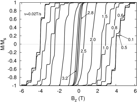
Figure 3: Simulated magnetic hysteresis loops ($M/M_{S}$ vs $B_{z}$) with sweeping rate $\nu=0.02$ T/s for ten temperatures: 0.1, 0.5, 0.6, 0.8, 1.0, 1.5, 2.0, 2.5, 2.8, and 3.2 K (from outside to inside). The lattice dimension is $10\times 10\times 10$. Note that the two curves of 0.1 K and 0.5 K fall in the same curve.

Presented in Fig. 4 are the right parts of the magnetization curves against the applied sweeping field for three temperatures, 0.1, 1.5, and 2.5 K, and with three sweeping rates, 0.002, 0.02, and 0.2 T/s. Here, the lattice dimension is $10\times 10\times 10$. We label a magnetization step by the magnetic field defined by its V-part near its vertex. For $T$=0.1K, only the direct LZ tunnelings change the magnetization, and the magnetization steps from $B_{z}$=2 to 6T in Fig. 4 correspond to $B_{S,m^{\prime}}^{0}$ with $m^{\prime}$ being from -6 to 2 in Table I. For $T$=1.5K, there are clear steps in the lower parts of the three magnetization curves, but their V-parts deviate substantially from the corresponding $B_{S,m^{\prime}}^{0}$ values and the steps are substantially deformed, which show that thermal-assisted LZ tunnelings play an important role. When temperature rises to 2.5K, there is no step structure and only one kink can be seen in the lower part of the magnetization curve in the cases of 0.2T/s and 0.02T/s. This is because the effects of thermal activation become dominating over the LZ tunneling effects. Different sweeping rates lead to substantial changes in the magnetization curves, and the larger the sweeping rate becomes, the larger the hysteresis loops are.

Figure 4: (Color online.) The right parts of simulated magnetization curves of different sweeping rates 0.002 (dot), 0.02 (dash), and 0.2 (solid) T/s for three temperatures 0.1 K, 1.5 K, and 2.5 K, as labelled. The lattice dimension is $10\times 10\times 10$. Each of the visible steps and kinks along a magnetization curve corresponds to one of the magnetic fields at which the direct and thermal assisted LZ tunnelings take place. The thin vertical dotted lines show the positions of $B_{S,m^{\prime}}^{0}$ for $m^{\prime}$=-10,-9,$\cdots$,2.

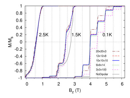
Figure 5: (Color online.) The right parts of simulated magnetization curves for three temperatures with five different lattice dimensions: $20\times 20\times 3$ (dash-dot), $12\times 12\times 8$ (dash), $10\times 10\times 10$ (solid), $9\times 9\times 14$ (dot), and $3\times 3\times 100$ (short-dash). The temperatures are 0.1 K, 1.5 K, and 2.5 K, as labelled. The sweeping rate is 0.02 T/s. For comparison, we also present the results without considering dipolar interaction (thin solid line).

Presented in Fig. 5 are the right parts of simulated hysteresis loops with $\nu$=0.02 T/s at three temperatures for five different lattice dimensions: $20\times 20\times 3$, $12\times 12\times 8$, $10\times 10\times 10$, $9\times 9\times 14$, and $3\times 3\times 100$. The temperatures are 0.1, 1.5, and 2.5 K. For comparison, the simulated results without the dipolar interaction are presented too. For $T$=0.1K, there are clear step structures for all the five lattice shapes. The step height varies with the lattice shape, which can be attributed to the dipolar interaction. If the dipolar interaction is switched off, there are only two steps: one tall step at $B_{z}=4.00$ T and the other very short step at 3.06 T. They correspond to the two transitions from 10 to -2 and -4, respectively. Other transitions from 10 to -4, -6, -8, and -10 have too small probabilities to be seen. When the dipolar interaction is switched on, the transition from 10 to -3 is allowed and the tall step becomes much shorter, resulting in the rich step structures between 3 and 6 T. The steps are caused by the direct LZ tunnelings. When the temperature changes to 1.5K, the hysteresis loops become substantially smaller because of the enhanced thermal effects. In this case, there are deformed step structures in the lower parts of the magnetization curves and there does not exists any clear step structure in the upper parts. The deformed step structures between 1 and 3 T result from the thermally assisted LZ tunnelings. For $T$=2.5K, there does not exist any step structure at all for all the six cases. The effect of the lattice shape is attributed to the long-range property of the dipolar interaction, and can be clearly seen in the magnetization curves only at the low temperatures in the extreme cases of $20\times 20\times 3$ and $3\times 3\times 100$. Actually, there is little visible difference between the magnetization curves of the three lattices: $12\times 12\times 8$, $10\times 10\times 10$, and $9\times 9\times 14$. Visible difference can be found at 0.1K and 1.5K only for the two extreme cases: $20\times 20\times 3$ and $3\times 3\times 100$. If we define a ratio $r=L_{l}/L_{t}$ of longitudinal size to transverse size for $L_{t}\times L_{t}\times L_{l}$, we have $r$=1 for $10\times 10\times 10$, $r$=0.67 for $12\times 12\times 8$, $r$=1.56 for $9\times 9\times 14$, $r$=0.15 for $20\times 20\times 3$, and $r$=33 for $3\times 3\times 100$. Therefore, there is little clear effect of lattice shape as long as the shape parameter $r$ is neither extremely large nor extremely small.

Now we address the statistical errors. We have calculated standard errors $\sigma_{M}$ of the reduced magnetization $M/M_{s}$ as functions of the sweeping field for various temperatures and sweeping rates. Our results show that for a given magnetization curve, the statistical errors are very small ($\sigma_{M}<0.005$) in the region of $B_{z}$ defined by $|M/M_{s}|>0.9$, and reach a maximal value $\sigma^{\rm max}_{M}$ near the point of $B_{z}$ defined by $M/M_{s}=0$. The maximal statistical error $\sigma^{\rm max}_{M}$ is dependent on the temperature and sweeping rate, varying from 0.015 to 0.025 for our simulation parameters. Such statistical errors appear only in a very small region of $B_{z}$. For any magnetization curve as a whole, the statistical errors are small enough to be acceptable.

Here we discuss effects of lattice sizes on simulated results. The above simulated results are based on the lattice dimensions: $20\times 20\times 3$, $12\times 12\times 8$, $10\times 10\times 10$, $9\times 9\times 14$, and $3\times 3\times 100$. They have $900\sim 1200$ body-centered unit cells, or $1800\sim 2400$ spins. To test our results, we have done a series of simulations for different parameters using lattice dimension defined by $L_{t}\times L_{t}\times L_{l}$. In the cases of $T=0.1$K, $\nu=0.2$T/s, and $L_{t}=L_{l}=L$ with $L=5\sim 20$, the largest size effects appear between 4 and 5.5 T for the right parts of the magnetization curves. For the steps at 4T, the $L$-caused change in the magnetization decreases quickly with increasing $L$, becoming very small when $L$ is larger than 9. Therefore, our lattice sizes of the results presented above are large enough to be reliable.

The above simulated results show that the area enclosed by a magnetization hysteresis loop decreases with the temperature increasing and increases with the sweeping rate increasing. This is completely consistent with the temperature and sweeping-rate dependence of the thermal reversal probability and LZ tunneling probabilities. Thermal activation effects dominate at high temperature. The LZ tunneling effects manifest themselves through the steps and kinks along the magnetization curves. However, there is a limit for the hysteresis loops at the low temperature end for a given sweeping rate. These limiting magnetization curves are caused by the minimal reversal probability set by the direct LZ quantum tunneling effect because the thermal activation probability becomes tiny at such low temperatures. With usual shape parameter $r$, these results are consistent with experimental magnetization curves of good Mn₁₂ crystal samples in the presence of little misalignments between the easy axis and applied fields Mn12tBuAc ; TB . In principle, a transverse magnetic field (due to the misalignment of the applied field and the easy axis) can enhance the energy splitting, and as a result will reduce the magnetization loop and smooth some steps Mn12tBuAc ; TB ; Mn12added . These usual (not extreme) shape parameters should reflect real shape factors in experimental samples. The consistence should be satisfactory, especially considering that our theoretical probabilities are calculated under leading order approximation and our model does not include possible defects and disorders in actual materials.

Table 1: Calculated results of $B_{S,m^{\prime}}^{0}$, $\Delta B^{n}_{S,m^{\prime}}$, $P_{S,m^{\prime}}^{0}$, $\langle P^{\rm LZ,n}_{S,m^{\prime}}\rangle$, and $\sigma_{S,m^{\prime}}^{n}$ for the direct LZ tunneling $(S,m^{\prime})$ when the field $B_{z}$ is swept to 3.75 T, where $n$ is determined by the field 3.75 T. $T=0.1$ K, $\nu=0.02$ T/s, and the lattice dimension is $10\times 10\times 10$.

$m^{\prime}$	$B_{S,m^{\prime}}^{0}$(T)	$\Delta B^{n}_{S,m^{\prime}}$(T)	$P_{S,m^{\prime}}^{0}$	$\langle P^{\rm LZ,n}_{S,m^{\prime}}\rangle$	$\sigma_{S,m^{\prime}}^{n}$
-10	0.000000	6.4$\times 10^{-15}$	0.00000	0.00000	0.00000
-9	0.564160	1.6$\times 10^{-6~{}}$	0	0.00000	0.00000
-8	1.099966	3.5$\times 10^{-6~{}}$	0.00000	0.00000	0.00000
-7	1.612415	5.1$\times 10^{-6~{}}$	0	0.00000	0.00000
-6	2.106511	6.7$\times 10^{-6~{}}$	0.00138	0.00138	0.00001
-5	2.587260	7.9$\times 10^{-6~{}}$	0	0.00002	0.00002
-4	3.059671	8.6$\times 10^{-6~{}}$	0.01815	0.01838	0.00320
-3	3.528757	8.6$\times 10^{-6~{}}$	0	0.22194	0.21086
-2	3.999529	7.8$\times 10^{-6~{}}$	1.00000	1.00000	0.00000
-1	4.476997	6.3$\times 10^{-6~{}}$	0	0.53746	0.33455
0	4.966165	3.9$\times 10^{-6~{}}$	1.00000	1.00000	0.00089
1	5.472035	7.4$\times 10^{-7~{}}$	0	0.99975	0.01091
2	5.999604	3.6$\times 10^{-6~{}}$	1.00000	1.00000	0.00000
3	6.553867	8.6$\times 10^{-6~{}}$	0	0.99988	0.00749

V Key roles of dipolar fields

To investigate the effects of dipolar interactions, we divide the dipolar fields within the $n$-th MC step, $(B_{ix,n}^{\rm di},B_{iy,n}^{\rm di},B_{iz,n}^{\rm di})$, into two parts: transverse dipolar field $B_{ix,n}^{\rm di}$ and $B_{iy,n}^{\rm di}$, and longitudinal dipolar field $B_{iz,n}^{\rm di}$. Transverse dipolar field not only modifies $B^{i,n}_{m,m^{\prime}}$, but also affects $\Delta^{i,n}_{m,m^{\prime}}$ and $P^{\rm LZ,i,n}_{m,m^{\prime}}$. In contrast, longitudinal dipolar field affects neither $\Delta^{i,n}_{m,m^{\prime}}$ nor $P^{\rm LZ,i,n}_{m,m^{\prime}}$, but shifts $B^{i,n}_{m,m^{\prime}}$ by $-B_{iz,n}^{\rm di}$. This means that LZ tunnelings actually occur at the field $B^{i,n}_{m,m^{\prime}}-B_{iz,n}^{\rm di}$, not $B^{i,n}_{m,m^{\prime}}$. This shift has two effects. First, it broadens the LZ transition and deforms the steps in magnetization curves. Second, the quick changing of $B_{iz,n}^{\rm di}$ results in that the value $B^{i,n}_{m,m^{\prime}}$ can be missed by the effective field $B_{z}+B_{iz,n}^{\rm di}$, and therefore the actual percentage of the reversed spins due to the LZ tunneling effect with respect to the total spins is smaller than the LZ probability $P^{\rm LZ,i,n}_{m,m^{\prime}}$ given in Eq. (12). This means that the dipolar interaction hinders both the direct LZ tunneling process and the thermal assisted LZ tunneling processes.

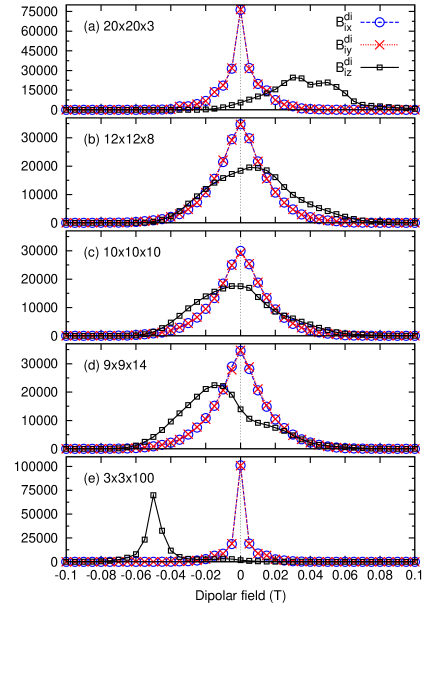
Figure 6: (Color online.) Distributions of dipolar fields $B_{ix}^{\rm di}$ (dashed line + circle), $B_{iy}^{\rm di}$ (dotted line + cross), and $B_{iz}^{\rm di}$ (solid line + square) for the five lattice dimensions $20\times 20\times 3$ (a), $12\times 12\times 8$ (b), $10\times 10\times 10$ (c), $9\times 9\times 14$ (e), and $3\times 3\times 100$ (e) when the field $B_{z}$ is swept to 3.75 T. The temperature $T$ is 0.1 K and the sweeping rate $\nu$ equals 0.02 T/s.

Without transverse dipolar field, $B_{m,m^{\prime}}^{i,n}$ becomes $B_{m,m^{\prime}}^{0}$, and $P^{\rm LZ,i,n}_{S,m^{\prime}}$ equals 0 for odd $m^{\prime}$ values because transverse dipolar field is the only transverse term of odd order in Hamiltonian Eq. (4). Without longitudinal dipolar field, the V-parts of steps remain vertical and the percentage of the reversed spins due to LZ tunneling is strictly equivalent to the LZ probability $P^{\rm LZ,i,n}_{S,m^{\prime}}$ at low temperatures. These are shown by the thin solid line for 0.1K in Fig. 5. In Table I we also present the average value ($\Delta B^{n}_{S,m^{\prime}}$=$\langle|B^{n}_{S,m^{\prime}}-B_{S,m^{\prime}}^{0}|\rangle$) of dipolar-field fluctuations with respect to $B_{S,m^{\prime}}^{0}$, the dipolar-field-free LZ probability $P^{0}_{S,m^{\prime}}$, and the average value $\langle P^{\rm LZ,n}_{S,m^{\prime}}\rangle$ and the corresponding standard error $\sigma_{S,m^{\prime}}^{n}$ of $P^{\rm LZ,i,n}_{S,m^{\prime}}$ for the avoided crossing positions of $S$ and $m^{\prime}$, where $m^{\prime}$ varies from -10 to 3 and the averaging $\langle X^{n}\rangle$ of $X^{i,n}$ is calculated over all the spins and all the runs within the $n$-th MC step. It should be pointed out that the $\Delta B^{n}_{S,m^{\prime}}$ values, although very important to LZ tunnelings, are very small, as shown in Table I. It is transverse dipolar field that make $\Delta B^{n}_{S,m^{\prime}}$ nonzero and make $P^{\rm LZ,i,n}_{S,m^{\prime}}$ ($m^{\prime}$=-5, -3, -1, 1, 3) change from 0 to nonzero, even nearly reach 1 in the cases $m^{\prime}=1$ and 3.

In order to elucidate the magnitude and distribution of the dipolar fields, we address the time-dependent distributions of SMMs that have dipolar fields $(B_{ix}^{\rm di},B_{iy}^{\rm di},B_{iz}^{\rm di})$ (here the continuous time variable is implied), or in short the distributions of $B_{ix}^{\rm di}$, $B_{iy}^{\rm di}$, and $B_{iz}^{\rm di}$, in the following. In Fig. 6 we compare the results from five different lattice dimensions: $20\times 20\times 3$, $12\times 12\times 8$, $10\times 10\times 10$, $9\times 9\times 14$, and $3\times 3\times 100$. Here the time is when the field $B_{z}$ is swept to 3.75 T, the temperature $T$ is 0.1 K, and the sweeping rate $\nu$ equals 0.02 T/s. For all the five lattices, our results show that the distribution of $B_{ix}^{\rm di}$ always is approximately equivalent to that of $B_{iy}^{\rm di}$ and they are both symmetrical and peaked at zero. The peak is sharper for the extremely slab-like $20\times 20\times 3$ lattice and extremely rod-like $3\times 3\times 100$ lattice. The peak of the $B_{iz}^{\rm di}$ distribution is wider than that of both $B_{ix}^{\rm di}$ and $B_{iy}^{\rm di}$. It shifts substantially away from zero when the lattice shape is either extremely slab-like or extremely rod-like. The leftward shift of the $B_{iz}^{\rm di}$ peak can be attributed to dipolar-interaction-induced ferromagnetic orders in rod-like systems garanin1 ; garanin2 , and the similar rightward shift to dipolar-interaction-induced antiferromagnetic orders in slab-like systems. Because dipolar interactions are the only inter-SMM interactions in our model, the differences of distributions between the the five lattices are caused by the dipolar fields, or dipolar interactions in essence.

VI conclusion

In summary, we have combined the thermal effects with the LZ quantum tunneling effects in a DMC framework by using the giant spin approximation for spins of SMMs and considering magnetic dipolar interactions for comparison with experimental results. We consider ideal lattices of SMMs consistent with experimental ones and assume that there are no defects and axis-misalignments therein. We calculate spin reversal probabilities from thermal-activated barrier hurdling, direct LZ tunneling effect, and thermal-assisted LZ tunneling effects in the presence of sweeping magnetic fields. Taking the parameters of experimental Mn₁₂ crystals, we do systematical DMC simulations with various temperatures and sweeping rates. Our results show that the step structures can be clearly seen in the low-temperature magnetization curves, the thermally activated barrier hurdling becomes dominating at high temperature near 3K, and the thermal-assisted tunneling effects play important roles at the intermediate temperature. These are consistent with corresponding experimental results on good Mn₁₂ samples (with less disorders) in the presence of little misalignments between the easy axis and applied fields Mn12tBuAc ; TB , and therefore our magnetization curves are satisfactory.

Furthermore, our DMC results show that the magnetic dipolar interactions, with the thermal effects, have important effects on the LZ magnetization tunneling effects. Their longitudinal parts can partially break the resonance conditions of the LZ tunnelings and their transverse parts can modify the tunneling probabilities. They can clearly manifest themselves when the SMM crystal is extremely rod-like or slab-like. However, both the magnetic dipolar interactions and the LZ tunneling effects have little effects on the magnetization curves when the temperature is near 3K. This DMC approach can be applicable to other SMM systems, and could be used to study other properties of SMM systems.

- (1) A. R. Rocha, V. M. García-suárez, S. W. Bailey, C. J. Lambert, J. Ferrer, and S. Sanvito, Nature Mater. 4, 335 (2005).
- (2) L. Bogani and W. Wernsdorfer, Nature Mater. 7, 179 (2008).
- (3) M. N. Leuenberger and D. Loss, Nature 410, 789 (2001).
- (4) M. Mannini, F. Pineider, P. Sainctavit, C. Danieli, E. Otero, C. Sciancalepore, A. M. Talarico, M.-A. Arrio, A. Cornia, D. Gatteschi, and R. Sessoli, Nature Mater. 8, 194 (2009).
- (5) C. Timm and F. Elste, Phys. Rev. B 73, 235304 (2006).
- (6) S. J. Koh, Nanoscale Res. Lett. 2, 519 (2007).
- (7) S. Barraza-Lopez, K. Park, V. Garcia-Suarez, and J. Ferrer, Phys. Rev. Lett. 102, 246801 (2009).
- (8) T. Lis, Acta Crystallogr., Sect. B 36, 2042 (1980).
- (9) R. Sessoli, D. Gatteschi, A. Caneschi, and M. A. Novak, Nature 365, 141 (1993).
- (10) L. Thomas, F. Lionti, R. Ballou, D. Gatteschi, R. Sessoli, and B. Barbara, Nature 383, 145 (1996).
- (11) J. R. Friedman, M. P. Sarachik, J. Tejada, and R. Ziolo, Phys. Rev. Lett. 76, 3830 (1996).
- (12) J. R. Friedman, M. P. Sarachik, J. Tejada, J. Maciejewski, and R. Ziolo, J. Appl. Phys. 79, 6031 (1996).
- (13) D. A. Garanin and E. M. Chudnovsky, hys. Rev. B 56, 11102 (1997).
- (14) I. Chiorescu, R. Giraud, A. G. M. Jansen, A. Caneschi, and B. Barbara, Phys. Rev. Lett. 85, 4807 (2000).
- (15) W. Wernsdorfer, M. Murugesu, and G. Christou, Phys. Rev. Lett. 96, 057208 (2006).
- (16) B. Barbara, L. Thomas, F. Lionti, I. Chiorescu, and A. Sulpice, J. Magn. Magn. Mater. 200, 167 (1999).
- (17) W. Wernsdorfer, S. Bhaduri, A. Vinslava, and G. Christou, Phys. Rev. B 72, 214429 (2005).
- (18) D. Gatteschi, R. Sessoli, and J. Villain, Molecular nanomagnets, Oxford University Press, New York 2006.
- (19) A. L. Barra, D. Gatteschi, and R. Sessoli, Phys. Rev. B 56, 8192 (1997).
- (20) A. Cornia, R. Sessoli, L. Sorace, D. Gatteschi, A. L. Barra, and C. Daiguebonne, Phys. Rev. Lett. 89, 257201 (2002).
- (21) L. Landau, Phys. Z. Sowjetunion 2, 46 (1932).
- (22) C. Zener, Proc. R. Soc. London, Ser. A 137, 696 (1932).
- (23) H. De Raedt, S. Miyashita, K. Saito, D. Garcia-Pablos, and N. Garcia, Phys. Rev. B 56, 11761 (1997).
- (24) Q. Niu and M. G. Raizen, Phys. Rev. Lett. 80, 3491 (1998).
- (25) N. V. Vitanov and K.-A. Suominen, Phys. Rev. A 59, 4580 (1999).
- (26) W. Wernsdorfer, R. Sessoli, A. Caneschi, D. Gatteschi, and A. Cornia, Europhys. Lett. 50, 552 (2000).
- (27) V. L. Pokrovsky and N. A. Sinitsyn, Phys. Rev. B 65, 153105 (2002).
- (28) Z.-D. Chen, J.-Q. Liang, and S.-Q. Shen, Phys. Rev. B 66, 092401 (2002).
- (29) M. Jona-Lasinio, O. Morsch, M. Cristiani, N. Malossi, J. H. Muller, E. Courtade, M. Anderlini, and E. Arimondo, Phys. Rev. Lett. 91, 230406 (2003).
- (30) Y.-C. Su and R. B. Tao, Phys. Rev. B 68, 024431 (2003).
- (31) C. Wittig, J. Phys. Chem. B 109, 8428 (2005).
- (32) E. Rastelli and A. Tassi, Phys. Rev. B 64, 064410 (2001).
- (33) P. Földi, M. G. Benedict, J. M. Pereira, Jr., and F. M. Peeters, Phys. Rev. B 75, 104430 (2007).
- (34) H. C. Kang and W. H. Weinberg, J. Chem. Phys. 90, 2824 (1989).
- (35) K. A. Fichthorn and W. H. Weinberg, J. Chem. Phys. 95, 1090 (1991).
- (36) G.-B. Liu and B.-G. Liu, Appl. Phys. Lett. 95, 183110 (2009).
- (37) A. Cornia, A. C. Fabretti, R. Sessoli, L. Sorace, D. Gatteschi, A.-L. Barra, C. Daiguebonned, and T. Roisnele, Acta Crystallogr., Sect. C 58, m371 (2002).
- (38) T. A. Witten and L. M. Sander, Phys. Rev. Lett. 47, 1400 (1981).
- (39) M. C. Bartelt and J. W. Evans, Phys. Rev. B 46, 12675 (1992).
- (40) C. Ratsch, P. Smilauer, A. Zangwill, and D. D. Vvedensky, Surf. Sci. 329, L599 (1995).
- (41) B.-G. Liu, J. Wu, E. G. Wang, and Z.Y. Zhang, Phys. Rev. Lett. 83, 1195 (1999).
- (42) J. W. Evans, P. A. Thiel, and M. C. Bartelt, Surf. Sci. Rep. 61, 1 (2006).
- (43) R. J. Glauber, J. Math. Phys. (N.Y.) 4, 294 (1963).
- (44) G. Korniss, J. White, P. A. Rikvold, and M. A. Novotny, Phys. Rev. E 63, 016120 (2000).
- (45) K. Park, P. A. Rikvold, G. M. Buendia, and M. A. Novotny, Phys. Rev. Lett. 92, 015701 (2004).
- (46) Y. Li and B.-G. Liu, Phys. Rev. Lett. 96, 217201 (2006).
- (47) Y. Li and B.-G. Liu, Phys. Rev. B 73, 174418 (2006).
- (48) B.-G. Liu, K.-C. Zhang, and Y. Li, Front. Phys. China 2, 424 (2007).
- (49) R. D. Kirby, J. X. Shen, R. J. Hardy, and D. J. Sellmyer, Phys. Rev. B 49, 10810 (1994).
- (50) W. Wernsdorfer, N. E. Chakov, and G. Christou, 70, 132413 (2004).
- (51) D. A. Garanin and E. M. Chudnovsky, Phys. Rev. B 78, 174425 (2008).
- (52) D. A. Garanin, Phys. Rev. B 80, 014406 (2009).