Abstract

Background

Empirical substitution matrices represent the average tendencies of substitutions over various protein families by sacrificing gene-level resolution. We develop a codon-based model, in which mutational tendencies of codon, a genetic code, and the strength of selective constraints against amino acid replacements can be tailored to a given gene. First, selective constraints averaged over proteins are estimated by maximizing the likelihood of each 1-PAM matrix of empirical amino acid (JTT, WAG, and LG) and codon (KHG) substitution matrices. Then, selective constraints specific to given proteins are approximated as a linear function of those estimated from the empirical substitution matrices.

Results

Akaike information criterion (AIC) values indicate that a model allowing multiple nucleotide changes fits the empirical substitution matrices significantly better. Also, the ML estimates of transition-transversion bias obtained from these empirical matrices are not so large as previously estimated. The selective constraints are characteristic of proteins rather than species. However, their relative strengths among amino acid pairs can be approximated not to depend very much on protein families but amino acid pairs, because the present model, in which selective constraints are approximated to be a linear function of those estimated from the JTT/WAG/LG/KHG matrices, can provide a good fit to other empirical substitution matrices including cpREV for chloroplast proteins and mtREV for vertebrate mitochondrial proteins.

Conclusions/Significance

The present codon-based model with the ML estimates of selective constraints and with adjustable mutation rates of nucleotide would be useful as a simple substitution model in ML and Bayesian inferences of molecular phylogenetic trees, and enables us to obtain biologically meaningful information at both nucleotide and amino acid levels from codon and protein sequences.

Introduction

Any method for inferring molecular phylogeny is implicitly or explicitly based on the evolutionary mechanism of nucleotide or amino acid substitutions, and the reliability of phylogenetic analyses strongly depends on models assumed for the substitution processes of nucleotide and amino acid. Mutational events occur at the individual nucleotide level, but selective pressure primarily operates at the amino acid level. Thus, a codon-based model of amino acid substitutions has a potential to be preferable to both mononucleotide substitution models [1, 2, 3] and amino acid substitution models [4, 5, 6, 7, 8, 9, 10, 11, 12], because it can take into account both mutational tendencies at the nucleotide level and selective pressure on amino acid replacements as well as the knowledge of a genetic code. Schneider et al. [13] and Kosiol et al. [14] empirically estimated a codon substitution matrix from a large number of coding sequence alignments. However, the tendencies of substitutions differ among nuclear, mitochondrial [6], and chloroplast genes [8]. Delport et al. [15, 16] pointed out that empirical substitution matrices represent the average tendencies of substitutions over various protein families by sacrificing gene-level resolution. A mechanistic codon substitution model, in which one can change a genetic code, and adjust mutational tendencies at the codon level and selectional preferences on amino acid replacements, is potentially more superior than empirical codon substitution matrices.

A main difference between the current mechanistic codon substitution models [17, 18, 19, 7, 20, 21, 22, 23, 24, 15, 16] resides in the estimation of selective constraints against amino acid replacements. (1) In [19, 20, 22], the difference between nonsynonymous and synonymous substitution rates was taken into account but the amino acid dependences of selective constraints were not taken into account; i.e., single selective constraints. (2) In [17, 18, 7], selective constraints against amino acid replacements were evaluated from physico-chemical properties of amino acids. (3) In [21, 23, 24], codon exchangeabilities for nonsynonymous changes were evaluated from those in empirical amino acid substitution matrices. (4) In [15, 16], selective constraints were grouped, and the number of groups and the strength of selective constraint of each group were optimized for a given protein phylogeny. The fourth method has the highest resolution of selective constraints employing as many substitution groups as necessary. However, it seems to be a very computer-intensive calculation [16]. Here, we try to estimate selective constraint for each type of amino acid replacement by maximizing the likelihood of individual empirical substitution matrices. Unlike the present method, in the previous methods of this third category codon exchangeabilities for nonsynonymous changes were assumed to be proportional to the corresponding amino acid exchangeability [23], or a codon substitution matrix was restricted to yield amino acid exchangeabilities equal to empirically-derived ones [21]. The empirical substitution matrices fitted are 1-PAM amino acid substitution frequency matrices, the JTT matrix [5], the WAG matrix [10], and the LG matrix [11], evaluated from relatively large data of nuclear-encoded proteins, the mtREV matrix [6] from vertebrate mitochondrial proteins, and the cpREV matrix [8] from chloroplast-encoded proteins, and also a 1-PAM codon substitution frequency matrix (KHG) [14]. In the following, these empirical substitution frequency matrices corresponding to 1 PAM will be simply referred to by their common acronyms, JTT, WAG, LG, KHG, mtREV, and cpREV.

In most of the reversible Markov models for codon substitutions, instantaneous rates for codon substitutions that require multiple nucleotide changes were assumed to be equal to $0$. [17, 18, 19, 15]. However, in all empirical substitution matrices unnegligible amounts of rates are assigned to amino acid replacements that require multiple nucleotide changes. Variations in substitution rates or time intervals would yield significant amounts of probabilities for the multi-step substitutions. Alternative explanation is that the significant fraction of these substitutions occurred with multiple nucleotide changes. Thus, both of them are taken into account in the present work. It is assumed that substitution rates are distributed with a $\Gamma$ distribution. The use of $\Gamma$ distribution for rate variation has been attempted in many studies [25, 26]. Multiple nucleotide changes are assumed to occur in the same order of time as single nucleotide changes do.

Interdependence of nucleotide substitutions at three codon positions [7] and also spanning codon boundaries [20] have been pointed out. Evidences for a high frequency, which is the order of 0.1 per site per billion years, of double-nucleotide substitutions were found in diverse organisms by Averof et al. [27], although there is a report [28] indicating a low rate of double-nucleotide mutations in primates. Bazykin et al. [29] pointed out a possibility of successive single compensatory substitutions for multiple nucleotide changes. Recently, many codon models relaxing mathematical assumptions in a more sophisticated way than the models of Goldman and Yang [18] and Muse and Gaut [19] are devised to study and to detect evidence of positive selection in codon evolutionary processes; see Anisimova and Kosiol [30] for a review.

In the Singlet-Doublet-Triplet (SDT) mutation model [20], single-nucleotide, doublet and triplet mutations spanning codon boundaries are taken into account, but double nucleotide mutations at the first and the third positions in a codon were not taken into account. The dependences of selective constraints on amino acid pairs were not taken into account. In the present model, it is assumed that nucleotide mutations occur independently at each codon position and so any double nucleotide mutation occurs as frequently as doublet mutations. The codon substitution rate matrix of KHG [14] indicates that some types of double nucleotide mutations at the first and the third positions frequently occur.

Close relationships between selective constraints on amino acids and physico-chemical properties of amino acids and protein structures have been pointed out [4, 31, 32, 17, 9, 33, 34]. We suppose that the relative strengths of selective constraints among amino acid pairs do not strongly depend on species, organelles, and even protein families but amino acid pairs. Then, we examine the performance of the present codon-based model, in which selective constraints are approximated to be a linear function of those estimated from JTT, WAG, LG, or KHG, in respect of how well other empirical substitution matrices including cpREV and mtREV can be fitted by adjusting parameters such as mutational tendencies and the strength of selective constraints. It is shown that these maximum likelihood (ML) estimators of the selective constraints perform better than any physico-chemical estimation. It is also indicated that the present model yields good values of Akaike information criterion (AIC) for a phylogenetic tree of mitochondrial coding sequences in comparison with the codon model almost equivalent to mtREV. If the present model is applied to the ML inference of phylogenetic trees, it will allow us to estimate mutational tendencies at the nucleotide level, which are specific to each species and organelle, such as transition-transversion bias and the ratio of nonsynonymous to synonymous rate. One of the interesting results revealed by the present model is that the ML estimators of transition to transversion bias calculated from the empirical substitution matrices are not so large as previously estimated. Also, AIC values indicate that a model allowing multiple nucleotide changes fits the empirical substitution matrices and the phylogeny of vertebrate mitochondrial proteins significantly better.

The present codon-based model with the new estimates for selective constraints on amino acids is useful as a simple evolutionary model for phylogenetic estimation, and also useful to generate log-odds for codon substitutions in protein-coding sequences with any genetic code.

Methods

A mechanistic codon substitution model with multiple nucleotide changes

In early codon substitution models [17, 18], the probabilities of multiple nucleotide replacements in the infinitesimal time difference $\Delta t$ were completely neglected by assuming them to be $O(\Delta t^{2})$, when the probabilities of single nucleotide replacements are taken to be $O(\Delta t)$. In other words, the instantaneous mutation rate $M_{\mu\nu}$ from codon $\mu$ to $\nu$ was assumed to be equal to zero for codon pairs requiring multiple nucleotide replacements. However, multiple nucleotide mutations may not be neglected in real protein evolution [35, 7, 27, 20, 29, 14]. Here, multiple nucleotide changes are assumed to occur with the same order of time as single nucleotide changes occur, but unlike the SDT model [20] a mutation process is simplified in such a way that mutations independently occur at each position of a codon. Thus, the mutation rate matrix for a codon is defined here as

$$M_{\mu\nu} \equiv \prod_{i=1}^{3}[\delta_{\mu_{i}\nu_{i}}+(1-\delta_{\mu_{i}\nu_{i}})(B_{i})_{\mu_{i}\nu_{i}}]\mbox{ for }\mu\neq\nu$$ (1)

where $B_{i}$ is a mutation rate matrix between the four types of nucleotides at the $i$th codon position, $\delta_{\mu_{i}\nu_{i}}$ is the Kronecker’s $\delta$, and the index $\mu_{i}$ means the $i$th nucleotide in the codon $\mu$; $\mu=(\mu_{1},\mu_{2},\mu_{3})$ where $\mu_{i}\in\mbox{\{ a, t, c, g \} }$. Assuming that the rate matrix $B_{i}$ satisfies the detailed balance condition, it is represented as

$$(B_{i})_{\mu_{i}\nu_{i}} = (m_{i})_{\mu_{i}\nu_{i}}f_{i,\nu_{i}}^{{\mbox{\scriptsize mut}}}\hskip 10.00002pt\mbox{ for }i=1,2,3$$ (2)

$$(m_{i})_{\mu_{i}\nu_{i}} = (m_{i})_{\nu_{i}\mu_{i}}$$ (3)

$$f^{{\mbox{\scriptsize mut}}}_{\nu=(\nu_{1},\nu_{2},\nu_{3})} = f_{1,\nu_{1}}^{{\mbox{\scriptsize mut}}}f_{2,\nu_{2}}^{{\mbox{\scriptsize mut}}}f_{3,\nu_{3}}^{{\mbox{\scriptsize mut}}}$$ (4)

where $f_{i,\nu_{i}}^{{\mbox{\scriptsize mut}}}$ is the equilibrium composition of nucleotide $\nu_{i}$ at the $i$th codon position, and $(m_{i})_{\mu_{i}\nu_{i}}$ is the exchangeability between nucleotides $\mu_{i}$ and $\nu_{i}$ at the $i$th codon position. As a result of the detailed balance condition assumed for the $B_{i}$, the $M$ also satisfies the detailed balance condition;

$$f_{\mu}^{{\mbox{\scriptsize mut}}}M_{\mu\nu} = f_{\nu}^{{\mbox{\scriptsize mut}}}M_{\nu\mu}$$ (5)

The instantaneous substitution rate $R_{\mu\nu}$ from codon $\mu$ to $\nu$ can be represented as the product of the mutation rate $M_{\mu\nu}$ and the average rate of fixation $F_{\mu\nu}$, which is defined to be the average fixation probability multiplied by the chromosomal population size, for mutations from codon $\mu$ to $\nu$ under selection pressure; $R_{\mu\nu}\propto\;M_{\mu\nu}F_{\mu\nu}\mbox{ for }\mu\neq\nu$. Let us assume that the $R$ also satisfies the detailed balance condition; that is,

$$f_{\mu}R_{\mu\nu} = f_{\nu}R_{\nu\mu}$$ (6)

where $f_{\mu}$ is the equilibrium codon composition of the substitution rate matrix $R$. The detailed balance condition Eq. 6 for the $R$ is equivalent with a condition that $R_{\mu\nu}$ can be expressed to be a product of the $(\mu,\nu)$ element of a symmetric matrix and the equilibrium composition $f_{\nu}$. Similarly, the detailed balance condition Eq. 5 for the $M$ is equivalent with a condition that the matrix whose ($\mu,\nu$) element is equal to $M_{\mu\nu}/f_{\nu}^{{\mbox{\scriptsize mut}}}$ is symmetric. Thus, the detailed balance conditions for the $M$ and the $R$ require that the average fixation rate $F_{\mu\nu}$ must be represented as the product of the two terms, $f_{\nu}/f_{\nu}^{{\mbox{\scriptsize mut}}}$ and $e^{w_{\mu\nu}}$, where $w_{\mu\nu}=w_{\nu\mu}$; $F_{\mu\nu}=(f_{\nu}/f_{\nu}^{{\mbox{\scriptsize mut}}})e^{w_{\mu\nu}}\;\mbox{ for }\mu\neq\nu$. Then, the codon substitution rate $R_{\mu\nu}$ can be represented as

$$R_{\mu\nu} = C_{{\mbox{\scriptsize onst}}}\;M_{\mu\nu}\frac{f_{\nu}}{f_{\nu}^{{\mbox{\scriptsize mut}}}}e^{w_{\mu\nu}}\;\mbox{ for }\mu\neq\nu$$ (7)

where $C_{{\mbox{\scriptsize onst}}}$ is an arbitrary scaling constant. By taking the frequencies of stop codons to be zero, the probability flow from any codon to a termination codon and its inverse flow are set to zero. The unit of time is chosen by determining the arbitrary scaling constant $C_{{\mbox{\scriptsize onst}}}$ in Eq. 7 in such a way that the total rate of the rate matrix $R$ is equal to one;

$$-\sum_{\mu}f_{\mu}R_{\mu\mu} = 1$$ (8)

Therefore, only the relative values among $M_{\mu\nu}$ are meaningful. The frequency-dependent term $f_{\nu}/f_{\nu}^{{\mbox{\scriptsize mut}}}$ represents the effects of selection pressures at the DNA level as well as at the amino acid level, which change the codon frequency from the mutational equilibrium frequency $f_{\nu}^{{\mbox{\scriptsize mut}}}$ to the frequency $f_{\nu}$ specific to a gene. The fixation rate is obviously equal to 0 for lethal mutations and 1 for neutral mutations. Here, we approximate the average quantity $e^{w_{\mu\nu}}$ over mutants to be independent of codon frequencies. The quantity $e^{w_{\mu\nu}}$ is the same as the one called the rate of acceptance by Miyata et al. [32]. We assume that selection pressure against codon replacements principally appears on an amino acid sequence encoded by a nucleotide sequence; $w_{\mu\nu}$ for the codon pair $(\mu,\nu)$ is equal to the selective constraint $w_{ab}$ for the encoded amino acid pair $(a,b)$.

$$e^{w_{\mu\nu}} \equiv \left\{\begin{array}[]{l}\sum_{a}\sum_{b\in\mbox{\{ amino acids \} }}C_{\mu a}C_{\nu b}e^{w_{ab}}\\ \ \hskip 20.00003pt\mbox{for }\hskip 10.00002pt\mu,\nu\notin\mbox{\{ stop codons \} and }\mu\neq\nu\\ 0\hskip 20.00003pt\mbox{for }\hskip 10.00002pt\mu\mbox{ or }\nu\in\mbox{\{ stop codons \} and }\mu\neq\nu\end{array}\right.$$ (12)

where $C_{\mu a}$ is a genetic code table and takes the value one if codon $\mu$ encodes amino acid $a$, otherwise zero. At the amino acid level, there should be no selection pressure against synonymous mutations. Thus, the $w_{ab}$ satisfies

$$w_{ab} = w_{ba}\hskip 10.00002pt,\hskip 10.00002ptw_{aa}=0$$ (13)

The matrix $w$ will be directly estimated by maximizing the likelihood of an empirical substitution matrix, or it will be evaluated for a specific protein family as a linear function of such an estimate of $w_{ab}$;

$$w_{ab} \equiv \beta w^{{\mbox{\scriptsize estimate}}}_{ab}+w_{0}(1-\delta_{ab})$$ (14)

In Eq. 14, $\delta_{ab}$ is the Kronecker’s $\delta$, and $w^{{\mbox{\scriptsize estimate}}}_{ab}$ means the estimate of $w_{ab}$, which is either a physico-chemical estimate or a ML estimate calculated from a specific substitution matrix, and satisfies Eq. 13. The parameter $\beta$, which is non-negative, adjusts the strength of selective constraints for a protein family. The parameter $w_{0}$ controls the ratio of nonsynonymous to synonymous substitution rate, but it will be ineffective and may be assumed to be equal to 0 if amino acid sequences rather than codon sequences are analyzed.

Then, the substitution probability matrix $S(t)$ at time t in a time-homogeneous Markov process can be calculated as

$$S(t)=\exp(Rt)$$ (15)

Because the rate matrix $R$ satisfies the detailed balance condition, the $S(t)$ also satisfies it. Therefore, a substitution process is modeled as a reversible Markov process. The $S(t)$ and the $R$ that satisfy the detailed balance condition can be easily diagonalized with real eigenvalues and eigenvectors [17]; the eigenvalues of $R$ are the same as those of a symmetric matrix whose $(\mu,\nu)$ element is equal to $(f_{\mu}/f_{\nu})^{1/2}R_{\mu\nu}$.

If multiple nucleotide changes were completely ignored, then Eq. 1 would be simplified as $M_{\mu\nu}=((1-\delta_{\mu_{1}\nu_{1}})(B_{1})_{\mu_{1}\nu_{1}}\delta_{\mu_{2}\nu_{2}}\delta_{\mu_{3}\nu_{3}})+(\delta_{\mu_{1}\nu_{1}}(1-\delta_{\mu_{2}\nu_{2}})(B_{2})_{\mu_{2}\nu_{2}}\delta_{\mu_{3}\nu_{3}})+(\delta_{\mu_{1}\nu_{1}}\delta_{\mu_{2}\nu_{2}}(1-\delta_{\mu_{3}\nu_{3}})(B_{3})_{\mu_{3}\nu_{3}})$, whose formulation for a codon mutation rate matrix with Eq. 2 is essentially the same as the one proposed by Muse and Gault [19]. Here, it should be noted that $(B_{i})_{\mu_{i}\nu_{i}}$ in Eq. 2 is defined to be proportional to the equilibrium nucleotide composition $f^{{\mbox{\scriptsize mut}}}_{i,\nu_{i}}$. Alternatively, one may define $M_{\mu\nu}$ as $M_{\mu\nu}=\prod_{i=1}^{3}[\delta_{\mu_{i}\nu_{i}}+(1-\delta_{\mu_{i}\nu_{i}})(m_{i})_{\mu_{i}\nu_{i}}]f^{{\mbox{\scriptsize mut}}}_{\nu}$ in the same way as Miyazawa and Jernigan [17] and others [18, 7] defined it to be proportional explicitly to the composition of the base triplet, $f^{{\mbox{\scriptsize mut}}}_{\nu}$. This alternative definition with Eqs. 7 and 8 is equivalent to Eqs. 1 and 2 with $f_{\nu_{i}}^{{\mbox{\scriptsize mut}}}=0.25$, and thus it is a special case in the present formulation; see [36] for justifications of this alternative definition.

In the present analyses, we assume for simplicity that $(m_{i})_{\mu_{i}\nu_{i}}$ and $f_{i,\nu_{i}}^{{\mbox{\scriptsize mut}}}$ do not depend on codon position $i$; that is, $(m_{i})_{\xi\eta}=m_{\xi\eta}$ and $f_{i,\xi}^{{\mbox{\scriptsize mut}}}=f_{\xi}^{{\mbox{\scriptsize mut}}}$, where $\xi,\eta\in\{a,t,c,g\}$. This assumption is reasonable because mutational tendencies may not depend on a nucleotide position in a codon. Let us define $m_{[tc][ag]}$ to represent the average of the exchangeabilities of the transversion type, $m_{ta}$, $m_{tg}$, $m_{ca}$, and $m_{cg}$, and likewise $m_{tc|ag}$ to represent the average of the exchangeabilities of the transition type, $m_{tc}$ and $m_{ag}$. We use the ratios $\{m_{\xi\eta}/m_{[tc][ag]}\}$ as parameters for exchangeabilities, and $m_{[tc][ag]}$ to represent the ratio of the exchangeability of double nucleotide change to that of single nucleotide change and also the ratio of the exchangeability of triple nucleotide change to that of double nucleotide change; note that the exchangeabilities of single, double, and triple nucleotide changes are of $O(m_{[tc][ag]}),O(m_{[tc][ag]}^{2})$, and $O(m_{[tc][ag]}^{3})$ in Eq. 1, respectively, and that Eq. 8 must be satisfied. Then, multiple nucleotide changes in a codon can be completely neglected by making the parameter $m_{[tc][ag]}$ approach zero with keeping $\{m_{\xi\eta}/m_{[tc][ag]}\}$ constant in Eq. 8. Also, it is noted that double nucleotide changes at the first and the third positions in a codon are assumed to occur as frequently as doublet changes.

Empirical substitution matrices used for model fitting

Maximum likelihood (ML) values are calculated for each 1-PAM substitution frequency matrix, which corresponds to the time duration of 1 amino acid substitution per 100 amino acids, of the JTT [5], the WAG [10], the LG [11], the cpREV [8], and the mtREV [6] amino acid substitution matrices, and of the KHG codon substitution matrix [14]. We have arbitrarily chosen the transition matrices of 1-PAM, whose time interval is long enough for the significant number of substitutions to occur and also too short for multi-step substitutions to cover multiple nucleotide changes. JTT is an accepted point mutation matrix compiled from the pairs of closely related proteins encoded in nuclear DNA. WAG, LG, cpREV, and mtREV are amino acid substitution matrices estimated by maximizing the likelihood of a given set of optimum phylogenetic trees. The KHG matrix used is the one named ECMunrest in the supplement of their paper, for which multiple nucleotide changes are allowed. JTT, WAG, LG, and KHG were all calculated from nuclear-encoded proteins, although JTT was calculated by a different method from the others. The matrices of cpREV and mtREV were calculated from proteins encoded in chloroplast DNA, and in vertebrate mitochondrial DNA, respectively. It should be noted here that a non-universal genetic code is used in the mitochondrial DNA.

Average of a transition matrix over time or over rate

In the present study, model parameters are estimated by maximizing the likelihood of each 1-PAM substitution frequency matrix of JTT, WAG, LG, cpREV, mtREV, and KHG. In the case of JTT, the pairs of closely related sequences were used to count substitutions and the transition matrix was calculated by completely neglecting multiple substitutions at a site in a parsimony method. Thus, JTT should be considered to consist of substitutions that occurred in various time intervals (various branch lengths). The substitution rate matrices of WAG, LG, mtREV, cpREV and KHG were estimated by the ML method for a given set of protein phylogenetic trees. Each site of protein families may have evolved with a different rate. As a result, these substitution matrices may be regarded as an average over different substitution rates. Here we assume that evolutionary time intervals or substitution rates for each substitution matrix are distributed in a $\Gamma$ distribution. There have been many attempts [25, 26] of using a $\Gamma$ distribution for rate variation.

If the substitution rate matrix $R$ is assumed to vary only by a scalar factor, the mean of a substitution matrix irrespective of over-time and over-rate will be calculated as

$$\langle S\rangle(\tau,\sigma)\equiv\int_{0}^{\infty}S(t)\Gamma(t;\tau,\sigma)dt$$ (16)

$$= \int_{0}^{\infty}\frac{1}{\Gamma(\tau)}\exp\{-(I-\sigma R)\frac{t}{\sigma}\}(\frac{t}{\sigma})^{\tau-1}\frac{dt}{\sigma}=[(I-\sigma R)^{-1}]^{\tau}$$

where $\Gamma(t;\tau,\sigma)$ is the probability density function of a $\Gamma$ distribution with a scale parameter $\sigma$ and a shape parameter $\tau$, $\Gamma(\tau)$ is the $\Gamma$ function, and $I$ is the identity matrix. The mean and the variance of the $\Gamma$ distribution $\Gamma(t;\tau,\sigma)$ are equal to $\tau\sigma$ and $\tau\sigma^{2}$, respectively. Here we should recall that the rate matrix $R$ is normalized such that the total rate per unit time is equal to one; see Eq. 8.

Evaluation of the log-likelihood of an empirical substitution matrix

The log-likelihood of the empirical frequency, $A_{\kappa\lambda}=Nf^{{\mbox{\scriptsize obs}}}_{\kappa}S^{{\mbox{\scriptsize obs}}}_{\kappa\lambda}$, of substitutions from $\kappa$ to $\lambda$ in the present model can be calculated as

$$\ell(\mbox{\boldmath{$\theta$}}) = N\sum_{\kappa}\sum_{\lambda}f^{{\mbox{\scriptsize obs}}}_{\kappa}S^{{\mbox{\scriptsize obs}}}_{\kappa\lambda}\log(f_{\kappa}\langle S\rangle(\tau,\sigma)_{\kappa\lambda})$$ (17)

where $\kappa$ and $\lambda$ mean one of the amino acid types for amino acid substitution matrices or one of the codon types for codon substitution matrices, $S^{{\mbox{\scriptsize obs}}}$ is an observed transition probability matrix corresponding to the accepted point mutation matrix $A$, $f^{{\mbox{\scriptsize obs}}}_{\kappa}$ is the observed composition of amino acid or codon $\kappa$, and $N$ is the total number of amino acid or codon sites compared to count substitutions. The observed composition $f^{{\mbox{\scriptsize obs}}}_{\kappa}$ is assumed to be the equilibrium composition of $S^{{\mbox{\scriptsize obs}}}$. $\theta$ is a set of parameters and $\hat{\mbox{\boldmath{$\theta$}}}=\arg\max_{\mbox{\boldmath{$\theta$}}}\ell(\mbox{\boldmath{$\theta$}})$ is a set of the maximum likelihood (ML) estimators. Similarly, the estimate $\hat{I}_{{\mbox{\scriptsize KL}}}$ of the Kullback-Leibler (K-L) information by replacing the real distribution to the observed frequency distribution is calculated as

$$\hat{I}_{{\mbox{\scriptsize KL}}}(\mbox{\boldmath{$\theta$}})$$ (18)

$$= \sum_{\kappa}\sum_{\lambda}f^{{\mbox{\scriptsize obs}}}_{\kappa}S^{{\mbox{\scriptsize obs}}}_{\kappa\lambda}[\log(f^{{\mbox{\scriptsize obs}}}_{\kappa}S^{{\mbox{\scriptsize obs}}}_{\kappa\lambda})-\log(f_{\kappa}\langle S\rangle(\tau,\sigma)_{\kappa\lambda})]$$

$$= -\ell(\mbox{\boldmath{$\theta$}})/N+\sum_{\kappa}\sum_{\lambda}f^{{\mbox{\scriptsize obs}}}_{\kappa}S^{{\mbox{\scriptsize obs}}}_{\kappa\lambda}\log(f^{{\mbox{\scriptsize obs}}}_{\kappa}S^{{\mbox{\scriptsize obs}}}_{\kappa\lambda})$$ (19)

Maximum log-likelihood $\ell(\hat{\mbox{\boldmath{$\theta$}}})$ corresponds to the minimum of the estimate of K-L information, $\hat{I}_{{\mbox{\scriptsize KL}}}(\hat{\mbox{\boldmath{$\theta$}}})$.

The transition probability, $S(t)_{ab}$, between amino acids $a$ and $b$ and the composition, $f_{a}$, of amino acid $a$ are related to those for codons as follows.

$$f_{a}S(t)_{ab} \equiv \sum_{\mu}\sum_{\nu}C_{\mu a}f_{\mu}S(t)_{\mu\nu}C_{\nu b}$$ (20)

$$f_{a} \equiv \sum_{\mu}C_{\mu a}f_{\mu}$$ (21)

The goodness of a model and the significance of parameters can be indicated by Akaike Information Criterion (AIC). The AIC value is defined as

AIC (22)

$$\equiv -2\ell(\hat{\mbox{\boldmath{$\theta$}}})+2\cdot(\mbox{number of adjustable parameters})$$

$$\Delta\mbox{AIC}$$ (23)

$$\equiv \mbox{AIC}+2N\sum_{\kappa}\sum_{\lambda}f^{{\mbox{\scriptsize obs}}}_{\kappa}S^{{\mbox{\scriptsize obs}}}_{\kappa\lambda}\log(f^{{\mbox{\scriptsize obs}}}_{\kappa}S^{{\mbox{\scriptsize obs}}}_{\kappa\lambda})$$

$$= 2N\hat{I}_{{\mbox{\scriptsize KL}}}(\hat{\mbox{\boldmath{$\theta$}}})+2\cdot(\mbox{number of adjustable parameters})$$ (24)

For convenience, $\Delta\mbox{AIC}$, which is equal to a constant value added to the AIC value, is also defined above. The AIC and $\Delta\mbox{AIC}$ always take a non-negative value. Models with smaller AIC and $\Delta\mbox{AIC}$ can be considered to be more appropriate [37].

Parameters in the present model are $\beta$, $m_{\xi\eta}$, $f_{\eta}^{{\mbox{\scriptsize mut}}}$, $f_{\eta}$, $\tau$, and $\sigma$. Assuming that the observed process of substitutions is in the stationary state, the estimates of the equilibrium codon and the equilibrium amino acid compositions, $\hat{f}_{\mu}$ and $\hat{f}_{a}$, are taken to be the observed composition of the codon and of the amino acid:

$$\hat{f}_{\mu} = f^{{\mbox{\scriptsize obs}}}_{\mu}\;,\hskip 20.00003pt\hat{f}_{a}=f^{{\mbox{\scriptsize obs}}}_{a}$$ (25)

In the case of amino acid sequences, for which their coding sequences are not available, codon compositions may be parameterized by

$$\hat{f}_{\mu} = \frac{\sum_{a}C_{\mu a}\hat{f}_{a}f_{\mu}^{{\mbox{\scriptsize usage}}}}{\sum_{a}C_{\mu a}\sum_{\nu}C_{\nu a}f_{\nu}^{{\mbox{\scriptsize usage}}}}$$ (26)

$$f^{{\mbox{\scriptsize usage}}}_{\nu=(\nu_{1},\nu_{2},\nu_{3})} = f_{\nu_{1}}^{{\mbox{\scriptsize usage}}}f_{\nu_{2}}^{{\mbox{\scriptsize usage}}}f_{\nu_{3}}^{{\mbox{\scriptsize usage}}}$$ (27)

In the present analyses, this parameterization is used for the equilibrium codon compositions in amino acid sequences.

Then, the shape parameter $\tau$ of a $\Gamma$ distribution for variations in mutation rates or evolutionary time intervals for observed codon or amino acid substitutions is estimated by equating the ratio of the expected number of substitutions in the model to its observed value.

$$\sum_{\kappa}\hat{f}_{\kappa}\langle S\rangle(\hat{\tau},\sigma)_{\kappa\kappa} = \sum_{\kappa}f^{{\mbox{\scriptsize obs}}}_{\kappa}S^{{\mbox{\scriptsize obs}}}_{\kappa\kappa}$$ (28)

Other parameters $\beta$, $m_{\xi\eta}$, $f_{\eta}^{{\mbox{\scriptsize mut}}}$, $f^{{\mbox{\scriptsize usage}}}_{\eta}$, and $\sigma$ are evaluated as ML estimators or fixed to a proper value. The observed transition matrix $S^{{\mbox{\scriptsize obs}}}_{\kappa\lambda}$ corresponding to 1-PAM is used here; PAM means accepted point mutations per 100 amino acids.

$$\sum_{a}f^{{\mbox{\scriptsize obs}}}_{a}S^{{\mbox{\scriptsize obs}}}_{aa} = 0.99$$ (29)

The total number of site comparisons ($N$) for each empirical substitution matrix

In the case of JTT, 59190 accepted point mutations found in 16130 protein sequences were used to build a substitution probability matrix of 1-PAM [5]. Thus, the total number $N$ of amino acid comparisons for JTT is assumed to be equal to $N=59190/0.01$. On the other hand, a phylogenetic tree for cpREV is based on $9957$ amino acid sites of 45 proteins encoded in chloroplast DNAs of 9 species [8], and the one for mtREV is based on $3357$ amino acid sites of the complete mitochondrial DNA from 20 vertebrate species (3 individuals from human) [6]. Thus, the total number of site comparisons $N$ for them may be approximated to be equal to the number of amino acid sites multiplied by the number of branches in the phylogenetic tree used to evaluate the transition matrices; that is, $N\approx 9957\cdot(2\cdot 10-3)=169269$ for cpREV, and $N\approx 3357\cdot(2\cdot 22-3)=137637$ for mtREV. The BRKALN database consisting of 50867 sites and 895132 residues was used to estimate WAG. Thus, $N\approx 895132\cdot 2-50867\cdot 3=1637663$ is used for WAG [10, 11]. To evaluate LG, 3412 of 3912 alignments consisting of 49637 sequences, 599692 sites, and 6697813 residues are used [11]. Therefore, $N\approx(6697813\cdot 2-599692\cdot 3)\cdot 3412/3912=$ $10114373$ is assumed for LG. These crude estimates of $N$ are used to evaluate the AICs of JTT, WAG, LG, cpREV and mtREV.

In the case of KHG, which was estimated by maximizing a likelihood of a set of phylogenetic trees of coding sequences of 7332 nuclear protein families taken from Pandit database [38], the total numbers of residues and sites are not written in Kosiol et al. [14], so that an AIC value is not given for KHG in the following.

Results

Models, each of which includes a different number of parameters and is a special case of models including more parameters, are fitted by a maximum likelihood method to each of the 1-PAM amino acid substitution frequency matrices, JTT [5], WAG [10], and LG [11] for proteins encoded in nuclear DNA, cpREV [8] for chloroplast DNA, and mtREV [6] for mitochondrial DNA. Also, the models are fitted to the 1-PAM codon substitution frequency matrix of KHG [14] for nuclear DNA. The selective constraints $w_{ab}$ are either directly estimated by ML or evaluated from a known estimate $w^{{\mbox{\scriptsize estimate}}}_{ab}$ by Eq. 14 that includes two parameters $\beta$ and $w_{0}$. The parameter $w_{0}$ is fixed here to $0$ for amino acid substitution matrices because the likelihood of an amino acid substitution matrix does not strongly depend on $w_{0}$; codon substitution data are required to reliably estimate the value of $w_{0}$, which significantly affects the ratio of nonsynonymous to synonymous substitution rate. Each model is named to indicate either the method to estimate $w_{ab}$ or the name of $w_{ab}^{{\mbox{\scriptsize estimate}}}$ with a suffix meaning the number of ML parameters. Each model is briefly described in Table 1. The Nelder-Mead Simplex algorithm has been used for the maximization of likelihoods.

The effects of selective constraints

First, the No-Constraints models, in which selective constraints do not depend on amino acid pairs, $\beta=0$ in Eq. 14, were examined to see how well nucleotide mutation rates, codon frequencies and a genetic code can explain the observed frequencies of amino acid substitutions in JTT, WAG, cpREV, and mtREV; the No-Constraints models disallowing multiple nucleotide changes are equivalent to mononucleotide substitution models, because $w_{0}=0$ is used here. The $\Delta\mbox{AIC}$ value and the ML estimates for each parameter set are listed in Table 2 and Table S1, respectively. Please refer to Supporting Information, Text S1, for details. These No-Constraints models serve as a reference to measure how selection models can improve the likelihoods. Then, we examine various estimations of selective constraints on amino acids based on the physico-chemical distances of amino acids evaluated by Grantham [31] and by Miyata et al. [32] and mean energy increments due to an amino acid substitution. These models are called Grantham, Miyata, and Energy-Increment-based (EI) models, respectively. Please refer to Supporting Information, Text S1, for the definition of the mean energy increment and for the details of each model. The $\Delta\mbox{AIC}$ values and the ML estimates for these models with various sets of parameters are also listed in Table 2, and Tables S2 and S3, respectively. Comparisons of $\Delta\mbox{AIC}$ values between the models in Table 2 indicate that the selective constraints on amino acids representing conservative selection against amino acid substitutions significantly improve the $\Delta\mbox{AIC}$ values of all substitution matrices. It is also indicated that the Miyata’s physico-chemical distance performs better in all parameter sets than the Grantham’s distance, This result is consistent with that of Yang et al. [7] for mitochondrial proteins. The present physico-chemical evaluation of selective constraints (EI models) fits JTT and WAG even better than the Miyata’s distance scale, although the performances of both the methods are almost same for cpREV and mtREV. One of the important facts in these results is that allowing multiple nucleotide changes in a codon significantly improve the AIC irrespective of the estimations of selective constraints; compare the $\Delta\mbox{AIC}$ values between the Grantham-10 and the Grantham-11, between the Miyata-10 and the Miyata-11, and between the EI-10 and the EI-11.

The effects of multiple nucleotide changes on ML estimations

In principle, all parameters $\{w_{ab}\}$ for selective constraints can be optimized in the case of codon sequences. In the case of protein sequences, all 190 non-diagonal elements of $w$ in addition to the parameters for mutational tendencies at the nucleotide level and others cannot simultaneously be optimized; the number of freedoms in a general reversible model for an amino acid transition matrix is equal to 209.

In order to see how well amino acid substitution matrices can be explained with the assumption of successive single nucleotide substitutions, let us optimize $w_{ab}$ corresponding to single-step amino acid pairs by assuming that only single nucleotide mutations are possible, i.e., by $m_{[tc][ag]}\rightarrow 0$ with $m_{\xi\eta}/m_{[tc][ag]}=\mbox{constant}$ in Eq. 8. The number of $w_{ab}$ for the single-step amino acid pairs is equal to 75 in the case of the universal genetic code. All 75 $w_{ab}$ for the single-step amino acid pairs have been optimized for each of JTT and WAG together with the nucleotide exchangeabilities $\{m_{\xi\eta}\}$, the equilibrium nucleotide composition $\{f^{{\mbox{\scriptsize mut}}}_{\xi}\}$, the codon usage parameters $\{f^{{\mbox{\scriptsize usage}}}_{\xi}\}$ and the scale parameter $\sigma$; the total number of the parameters is equal to 87 in addition to the 19 amino acid frequencies and the shape parameter $\tau$. This maximum likelihood model to estimate the matrix $w$ is called ML with a suffix meaning the number of ML parameters; see Table 1. The ML estimates of these parameters except $\hat{w}_{ab}$ for the ML-87 are listed in Table 3 for JTT and WAG.

In the lowest rows of this table, the ratio of the total nucleotide substitution rate per codon to the codon substitution rate, which represents the average number of nucleotide changes for substituting a codon, the ratio of the total transition to the total transversion rate per codon, and the ratio of nonsynonymous to synonymous substitution rate per codon are listed for the models. The sum of the total transition and the total transversion rates per codon is equal to the total nucleotide substitution rate per codon. The lowest three rows list their values in the case of $\sigma\rightarrow 0$ and $w_{ab}=0$, and the second lowest three rows for the case of $\sigma\rightarrow 0$. Thus, the differences of their values between the lowest and second lowest three rows represent the effects of selective constraints on amino acids ($w_{ab}$), and those between the second lowest and the third lowest three rows describe the effects of rate/time variations on the substitution matrix. If codon substitutions proceed by successive single nucleotide changes, i.e., $m_{[tc][ag]}\rightarrow 0$, then the ratio of the total nucleotide to the codon substitution rate will be equal to 1 in the case of $\sigma\rightarrow 0$.

Here it should be noticed that the nonsynonymous and the synonymous substitution rates are defined not to be rate per site but simply rate per codon. The sum of the nonsynonymous and the synonymous substitution rates is equal to the codon substitution rate. The ratio of the nonsynonymous to the synonymous substitution rate per codon does not corresponds to the ratio of nonsynonymous to synonymous substitutions per site, $K_{A}/K_{S}$ [39], but the ratio of nonsynonymous to synonymous substitutions per codon, $M_{A}/M_{S}$ [39]. The ratio ($N_{A}/N_{S}$ [39]) of the effective number of nonsynonymous sites to that of synonymous sites per codon corresponds to the ratio of nonsynonymous to synonymous rate in the case of no selective constraints ($w_{ab}=0$). In the present models, $K_{A}/K_{S}$ indicating the effects of selection on amino acid replacements corresponds to the nonsynonymous to synonymous substitution rate ratio in the case of $\sigma\rightarrow 0$ divided by that in the case of $w_{ab}=0$ and $\sigma\rightarrow 0$. Table 3 indicates that selection on amino acids is conservative, because the ratio of nonsynonymous to synonymous rate per codon is much smaller in the case of $\sigma\rightarrow 0$ than in the case of $w_{ab}=0$ and $\sigma\rightarrow 0$.

As expected, the AIC value drastically decreases from that of the EI-14 in both cases of JTT and WAG, indicating that the introduction of many parameters may be still appropriate. However, there are large discrepancies between the observed transition matrix and the one estimated by the ML-87. Let us see the discrepancies between them in terms of log-odds.

A log-odds matrix introduced by Dayhoff et al. [4] is one of the representations of amino acid substitution propensities. The $(\kappa,\lambda)$ element of the log-odds matrix is defined to be the logarithm of odds to find an amino acid pair $(\kappa,\lambda)$ in comparison with random sequences. The odds $O_{\kappa\lambda}$ is equal to the $(\kappa,\lambda)$ element of transition matrix divided by the amino acid composition $f_{\lambda}$.

$$O(S(t))_{\kappa\lambda} \equiv S(t)_{\kappa\lambda}/f_{\lambda}$$ (30)

$$\mbox{log-}O(S(t))_{\kappa\lambda} \equiv \frac{10}{\log 10}\log O(S(t))_{\kappa\lambda}$$ (31)

The proportional constant in Eq. 31 is the one originally used by Dayhoff et al. [4].

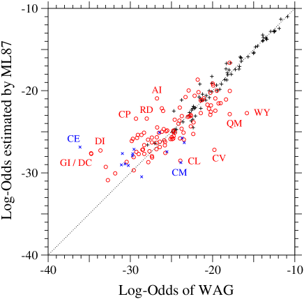
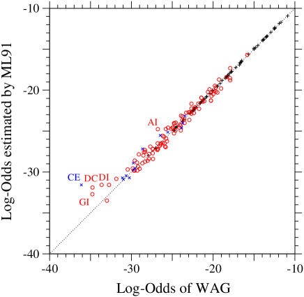
Figure S1: The ML-87 and the ML-91 models fitted to WAG. Each element log-$O(\langle S\rangle(\hat{\tau},\hat{\sigma}))_{ab}$ of the log-odds matrices of (A) the ML-87 and (B) the ML-91 models fitted to the 1-PAM WAG matrix is plotted against the log-odds log-$O(S^{{\mbox{\scriptsize WAG}}}(\mbox{1 PAM}))_{ab}$ calculated from WAG. Plus, circle, and cross marks show the log-odds values for one-, two-, and three-step amino acid pairs, respectively. The dotted line in each figure shows the line of equal values between the ordinate and the abscissa.

In Fig. 1, the log-odds $\mbox{log-}O(\langle S\rangle(t))_{ab}$ corresponding to the 1 PAM transition matrix of the ML-87 model fitted to JTT are plotted against those calculated from JTT. Plus, circle and cross marks show the log-odds for one-, two-, and three-step amino acid pairs, respectively. Although the estimated values of log-odds for one-step amino acid pairs are almost exactly equal to those of the JTT matrix, there are still large discrepancies between the log-odds values for two- and three-step amino acid pairs, indicating a non-stepwise manner of codon substitutions. Similar discrepancies are also found in Fig. S1 for WAG.

We have examined how the AIC is improved by enabling multiple nucleotide changes in a codon. The selective constraints $\{w_{ab}\}$ for multiple nucleotide changes are classified into 6 groups according to the amounts of discrepancies between the observed and the estimated values of the log-odds as shown in Fig. 1. Then, the ML estimates of 94 parameters including 7 additional parameters, $w_{ab}$ for the 6 groups of multiple nucleotide changes and the parameter $m_{[tc][ag]}$ for the rate of multiple nucleotide change, are calculated. This model is called ML-94. Also, the values of $\{w_{ab}\}$ for multi-step amino acid pairs are calculated by maximizing the likelihood with fixing the values of all other parameters including $w_{ab}$ for the single-step amino acid pairs; this model is called here ML-94+ by appending the ”+” mark. It should be noted that these values of $\hat{w}_{ab}$ for the multi-step amino acid pairs in the ML-94+ are not ML estimates at all. The ML estimates $\hat{w}_{ab}$ for single-step amino acid pairs, the classification of multi-step amino acid pairs into the 6 groups, and the ML estimates for those categories of $w_{ab}$ are provided in Supporting Information, Data S1. As shown in Table 3, the ML estimates of $m_{\xi\eta}$, $f^{{\mbox{\scriptsize mut}}}_{\xi}$, and $f^{{\mbox{\scriptsize usage}}}_{\eta}$ for the ML-87 model are very different from those for the ML-94, and some of them for the ML-87 seem to be unrealistic. For example, $\hat{m}_{ta}/\hat{m}_{[tc][ag]}$ is evaluated to be smaller than $0.1$. Also, the small value of $\hat{f}^{{\mbox{\scriptsize usage}}}_{t+a}$ indicates the extremely biased usage of codons. The ML estimate $\hat{\sigma}$ of a $\Gamma$ distribution is too large. These parameters are forced in the ML-87 to take such values to reduce the discrepancies between the observed and the estimated counts for multi-step amino acid pairs. In the ML-94 model, the ML estimators of these parameters take more reasonable values. However, it may also yield unreasonable estimates for codon usage parameters, $\{f^{{\mbox{\scriptsize usage}}}_{\xi}\}$; for example, $\hat{f}^{{\mbox{\scriptsize usage}}}_{t+a}=0.221$ in the ML-94 for WAG, and $\hat{f}^{{\mbox{\scriptsize usage}}}_{c}=0.249\cdot\hat{f}^{{\mbox{\scriptsize usage}}}_{c+g}=0.14$ in the ML-94 for LG. Thus, the ML-91 model with $f^{{\mbox{\scriptsize usage}}}_{\xi}=0.25$, which means equal codon usage, may be better than the ML-94. The ML-91 model was applied for JTT, WAG, and LG, and the ML estimates for them in the ML-91 are also listed in Table 3.

The ML estimators $\hat{m}_{\xi\eta}$, $\hat{f}^{{\mbox{\scriptsize mut}}}_{\xi}$, and $\hat{\sigma}$ show a similar tendency between the ML-91 models for all the amino acid substitution matrices, i.e., JTT, WAG, and LG. The parameter $m_{[tc][ag]}$ for multiple nucleotide changes and the scale parameter $\sigma$ for rate variation are both significant for all the matrices. The values of $\hat{m}_{tc|ag}/\hat{m}_{[tc][ag]}>1$ for JTT, WAG, and LG indicate that the mean exchangeability of the transition type is larger than that of the transversion type in all the matrices.

As shown in Fig. 1 for JTT and in Fig. S1 for WAG, the large discrepancies of the log-odds for the multi-step amino acid pairs disappear in the ML-91, in which multiple nucleotide changes are taken into account. The AIC values of JTT and WAG are significantly improved by enabling multiple nucleotide changes in the ML-91. This fact confirms that multiple nucleotide changes are statistically significant and should be taken into account to build a codon substitution model.

ML estimation for the KHG codon substitution matrix

If a codon substitution matrix is used for model fitting with the assumption of multiple nucleotide changes, all 190 parameters of selective constraints $\{w_{ab}\}$ will be able to be optimized. The ML-200 model has been fitted to the 1-PAM codon substitution frequency matrix of KHG, which was empirically estimated without any restriction on multiple nucleotide changes [14].

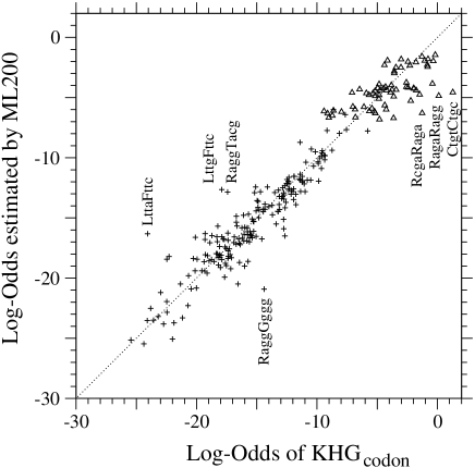
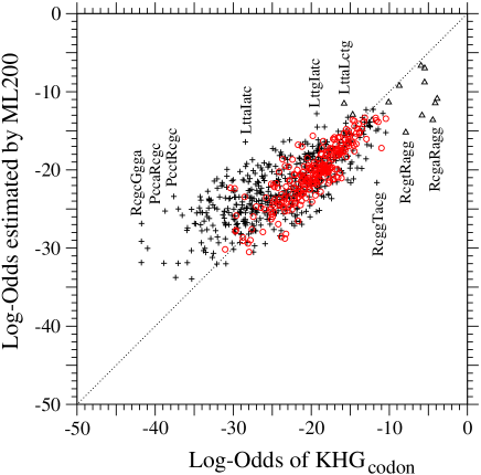
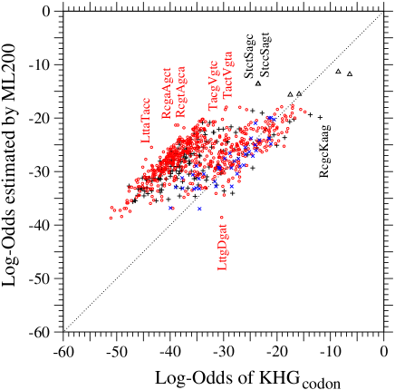
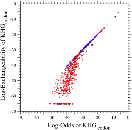
C                                                                                                                                                D

Figure 2: The ML-200 model fitted to KHG. Each element log-$O(\langle S\rangle(\hat{\tau},\hat{\sigma}))_{\mu\nu}$ of the log-odds matrix corresponding to (A) single, (B) double, and (C) triple nucleotide changes in the ML-200 model fitted to the 1-PAM KHG codon substitution matrix is plotted against the log-odds log-$O(S^{{\mbox{\scriptsize KHG}}}(\mbox{1 PAM}))_{\mu\nu}$ calculated from KHG. In (D), codon log-exchangeabilities of the 1-PAM KHG codon substitution matrix corresponding to triple nucleotide changes are plotted against the log-odds log-$O(S^{{\mbox{\scriptsize KHG}}}(\mbox{1 PAM}))_{\mu\nu}$ calculated from KHG. The log-exchangeability of the 1-PAM KHG is defined as $(10/\log 10)\log[R^{{\mbox{\scriptsize KHG}}}_{\mu\nu}\cdot t_{{\mbox{\scriptsize 1-PAM}}}/f_{\nu}]$. Upper triangle, plus, circle, and cross marks show the log-odds values for synonymous pairs and one-, two-, and three-step amino acid pairs, respectively. Log-exchangeabilities for the codon pairs whose instantaneous rates are estimated to be $0$ in KHG are shown to be about $-65$ in this figure. The dotted line in each figure shows the line of equal values between the ordinate and the abscissa.

The log-odds values for the codon pairs requiring single, double, and triple nucleotide changes are shown in Figs. 2A, 2B, and 2C, respectively. In these figures, upper triangle, plus, circle, and cross marks show the log-odds values for synonymous pairs and one-, two-, and three-step amino acid pairs, respectively. The dotted line shows the line of values where the observed and the estimated values of log-odds are equal to each other. The log-odds of the codon pairs requiring single/double/triple nucleotide changes for one/two/three-step amino acid pairs respectively tend to fall along the dotted line in comparison with the log-odds of the other codon pairs. In other words, the log-odds of the codon pairs for which any nucleotide change is accompanied by an amino acid change are correctly estimated. On the other hand, the estimated log-odds values do not well agree with the observed ones for synonymous codon pairs shown by the upper triangles. These estimated log-odds can be adjusted only by changing nucleotide mutation rates, i.e., $m_{\xi\eta}$ and $f^{{\mbox{\scriptsize mut}}}_{\xi}$. Thus, the approximations of the independence and of no difference of nucleotide exchangeabilities between nucleotide positions may be limited; see Eq. 1.

The codon pairs, whose log-odds values are less than $-30$ and which require more nucleotide changes than the least nucleotide changes required for the corresponding amino acid pair, tend to be located in the upper region than in the lower region of the dotted line; see plus marks in Fig. 2B and plus and circle marks in Fig. 2C. Such a tendency is more clear in Fig. 2C, in which plus and circle marks corresponding to one- and two-step amino acid pairs are mostly located far from and almost in parallel to the dotted line. The estimated values of the log-odds for these one- and two-step amino acid pairs are greater by 10 – 15 than the observed values.

In Fig. 2D, the log-exchangeabilities of the codon pairs requiring triple nucleotide changes in the 1-PAM KHG matrix are plotted against their log-odds of the 1-PAM KHG matrix. The log-exchangeability is defined here to be $(10/\log 10)\log[R^{{\mbox{\scriptsize KHG}}}_{\mu\nu}\cdot t_{{\mbox{\scriptsize 1-PAM}}}/f_{\nu}]$. The log-exchangeabilities of the codon pairs corresponding to three-step amino acid pairs are all nearly equal to their log-odds. The smallest log-exchangeabilities of these codon pairs reach almost $-40$. However, there are many codon pairs whose log-exchangeabilities are smaller than $-40$, and all of them correspond to one- or two-step amino acid pairs. The log-exchangeabilities of these codon pairs are significantly smaller than their log-odds, indicating that almost all substitutions of these codon pairs were estimated in KHG not to occur by triple nucleotide changes but rather by successive single or double nucleotide changes.

In the present model, codon exchangeabilities are approximated by the product of nucleotide exchangeabilities; see Eq. 1 for the exact expression. Therefore, all codon exchangeabilities for triple nucleotide changes are in the same order of magnitude, and specific codon pairs cannot be significantly less exchangeable. Thus, the present approximation for codon exchangeabilities may have a limitation, unless those exchangeabilities of KHG are underestimated. Estimation of the exchangeabilities for those codon pairs, which require more nucleotide changes than the least nucleotide changes required for the corresponding amino acid pair, may be less reliable than for the others.

The ML estimates $\hat{m}_{\xi\eta}$, $\hat{f}^{{\mbox{\scriptsize mut}}}_{\xi}$ and $\hat{\sigma}$ for KHG are listed in Table 3. The scale parameter $\sigma$ of the $\Gamma$ distribution is estimated to be $0.0$ for KHG, meaning that variations in rates need not be taken into account for KHG. There is a different tendency in the $\{\hat{m}_{\xi\eta}\}$ between KHG and the amino acid substitution matrices. One remarkable difference between them is that the parameter $m_{tc|ag}/m_{[tc][ag]}$ for transition-transversion bias is estimated to be greater than one in the ML-91 for JTT, WAG, and LG but to be less than one in the ML-200 for KHG. This estimation of transition to transversion bias for KHG results from a fact that the ratio of the total transition to the total transversion substitution rate is actually equal to $0.765$ in KHG, although this fact is contrary to the common understanding of transition-transversion bias. Because selective constraints on amino acids more favor transitions than transversions, transition-transversion bias in nucleotide mutation rates for KHG must be much less than $0.765$. Actually the ratio of the total transition to the total transversion mutation rate is estimated to be 0.427; see Table 3.

Comparison of ML estimates $\hat{w}_{ab}$ among the present models

In Table 4, the correlation coefficients of $\hat{w}_{ab}$ between the present models are listed. The lower half of the table lists those for single-step amino acid pairs, and the upper half lists those for multi-step amino acid pairs by excluding the amino acid pairs that belong to the least exchangeable class at least in one of the models. Each model name of JTT/WAG/LG-ML91+ and KHG-ML200 means the empirical substitution matrix and the method used to estimate selective constraints, $w_{ab}$. In the following, these ML estimates of $w_{ab}$ will be specified as $\hat{w}_{ab}^{{\mbox{\scriptsize JTT/WAG/LG-ML91+}}}$ and $\hat{w}_{ab}^{{\mbox{\scriptsize KHG-ML200}}}$. In the EI method, selective constraints are approximated by a linear function of the energy increment due to an amino acid substitution, $\Delta\hat{\varepsilon}^{{\mbox{\scriptsize c}}}_{ab}+\Delta\hat{\varepsilon}^{{\mbox{\scriptsize v}}}_{ab}$, which is defined by Eqs. S1-4, S1-5, and S1-6 in Supporting Information, Text S1; therefore, $\hat{w}_{ab}^{{\mbox{\scriptsize EI}}}\equiv-(\Delta\hat{\varepsilon}^{{\mbox{\scriptsize c}}}_{ab}+\Delta\hat{\varepsilon}^{{\mbox{\scriptsize v}}}_{ab})$.

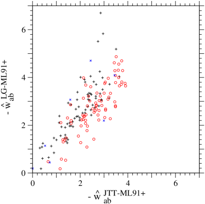
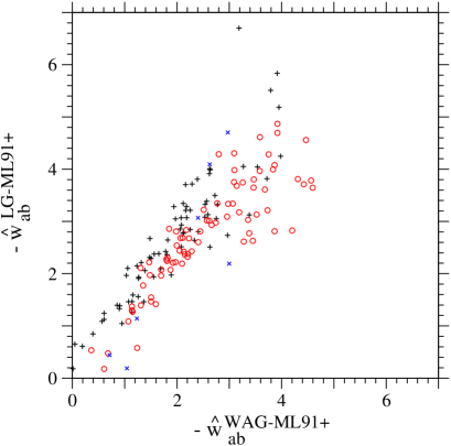
C                                                                                                                                          D

     

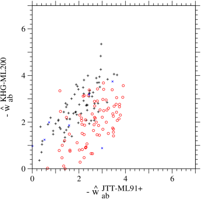
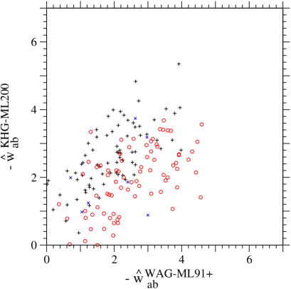
E                                                                                                                                          F

     

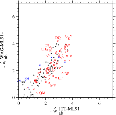
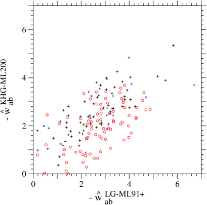
Figure S2: Comparison between various estimates of selective constraint for each amino acid pair The ML estimates of selective constraint on substitutions of each amino acid pair are compared between the models fitted to various empirical substitution matrices. The estimates $\hat{w}_{ab}$ for multi-step amino acid pairs that belong to the least exchangeable class at least in one of the models are not shown. Plus, circle, and cross marks show the values for one-, two-, and three-step amino acid pairs, respectively.

The correlations of the ML estimates $\{\hat{w}_{ab}\}$ between the JTT-ML91+, the WAG-ML91+, and the LG-ML91+ are very strong even for the multi-step amino acid pairs. Comparisons of the ML estimates of selective constraints between various models are shown in Fig. S2. The $\{\hat{w}_{ab}^{{\mbox{\scriptsize KHG-ML200}}}\}$ estimated from the KHG codon substitution matrix are less correlated with $\{\hat{w}_{ab}^{{\mbox{\scriptsize JTT/WAG/LG-ML91+}}}\}$ from the other amino acid substitution matrices, especially less for the multi-step amino acid pairs. The ML estimates $\{-\hat{w}_{ab}\}$ for the multi-step amino acid pairs are relatively smaller in the KHG-ML200 than in the JTT/WAG/LG-ML91+ models; see Fig. S2.

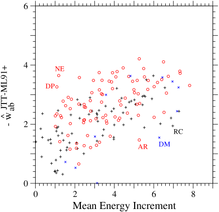
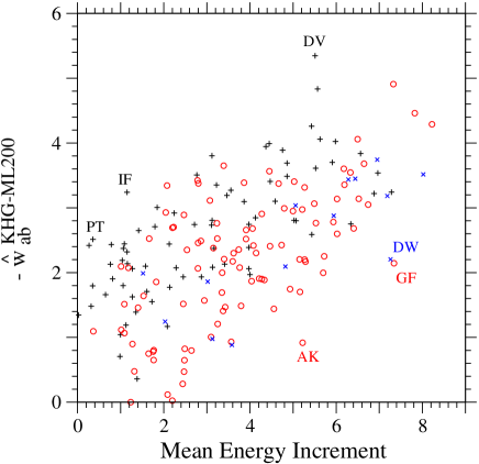
Figure 3: Selective constraint for each amino acid pair estimated from JTT and from KHG. The ML estimate, (A) $-\hat{w}^{{\mbox{\scriptsize JTT-ML91+}}}_{ab}$ in the ML-91+ model fitted to the 1-PAM JTT amino acid substitution matrix and (B) $-\hat{w}^{{\mbox{\scriptsize KHG-ML200}}}_{ab}$ in the ML-200 model fitted to the 1-PAM KHG codon substitution matrix, for each amino acid pair is plotted against the mean energy increment due to an amino acid substitution, ($\Delta\hat{\varepsilon}^{{\mbox{\scriptsize c}}}_{ab}+\Delta\hat{\varepsilon}^{{\mbox{\scriptsize v}}}_{ab}$) defined by Eqs. S1-4, S1-5, and S1-6 in Supporting Information, Text S1. In (A), the estimates $\hat{w}_{ab}$ for the least exchangeable class of multi-step amino acid pairs are not shown. Plus, circle, and cross marks show the values for one-, two-, and three-step amino acid pairs, respectively.

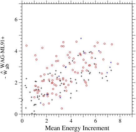
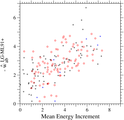
Figure S3: Selective constraint for each amino acid pair estimated from WAG and from LG. The ML estimate, $-\hat{w}^{{\mbox{\scriptsize WAG-ML91+}}}_{ab}$ in (A) and $-\hat{w}^{{\mbox{\scriptsize LG-ML91+}}}_{ab}$ in (B), of selective constraint on substitutions of each amino acid pair in the ML-91+ models fitted to the 1-PAM matrices of WAG and LG is plotted against the mean energy increment due to an amino acid substitution, ($\Delta\hat{\varepsilon}^{{\mbox{\scriptsize c}}}_{ab}+\Delta\hat{\varepsilon}^{{\mbox{\scriptsize v}}}_{ab}$) defined by Eqs. S1-4, S1-5, and S1-6. The estimates $\hat{w}_{ab}$ for the least exchangeable class of multi-step amino acid pairs are not shown. Plus, circle, and cross marks show the values for one-, two-, and three-step amino acid pairs, respectively.

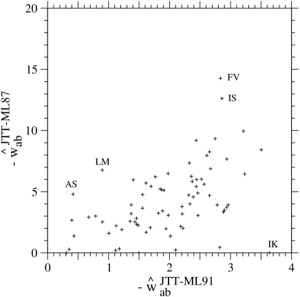
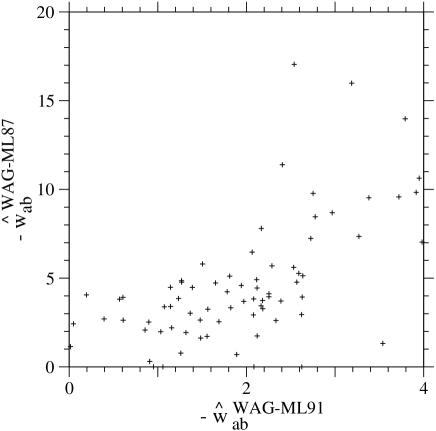
Figure S4: Comparison of the ML estimates of selective constraint for each amino acid pair between the ML-87 and the ML-91 models. The ML estimate of selective constraint for each single step amino acid pair in the ML-87 model fitted to (A) the 1-PAM JTT matrix or (B) the 1-PAM WAG matrix is plotted against that in the ML-91 model.

The correlations of $\{\hat{w}_{ab}\}$ between the EI and others are not as good as those between the other estimates, but they are significant especially between the EI and the KHG-ML200 even for the multi-step amino acid pairs. In Fig. 3A, the ML estimates $\{-\hat{w}_{ab}^{{\mbox{\scriptsize JTT-ML91+}}}\}$ in the JTT-ML91+ are plotted against the energy increments $\{-\hat{w}_{ab}^{{\mbox{\scriptsize EI}}}\}$ due to an amino acid substitution; the least exchangeable category of multi-step amino acid pairs are not shown in this figure. Similar plots for the WAG-ML91+ and for the LG-ML91+ are shown in Fig. S3. The ML estimates $\{-\hat{w}_{ab}^{{\mbox{\scriptsize KHG-ML200}}}\}$ for all amino acid pairs in the KHG-ML200 are plotted against the energy increments $\{-\hat{w}_{ab}^{{\mbox{\scriptsize EI}}}\}$ in Fig. 3B. No drastic difference in the correlation between these two quantities is found among one-, two-, and three-step amino acid pairs. The correlations of $\{\hat{w}_{ab}\}$ between the EI and the other models are better for the ML-91 than for the ML-87; the correlation coefficient between them for the single step amino acid pairs is equal to $0.19$ for the JTT-ML87 but $0.66$ for the JTT-ML91 and $0.30$ for the WAG-ML87 but $0.68$ for the WAG-ML91. The ML estimates $\{-\hat{w}_{ab}\}$ for the single step amino acid pairs are compared between the ML-87 and the ML-91 models in Fig. S4.

In the next section, we will examine whether the differences among these estimates of $w_{ab}$ are significant in representing selective constraints on amino acids.

Performance of the ML estimates $\{\hat{w}_{ab}\}$ and the characteristics of nucleotide mutations estimated

The present model for codon substitutions is designed to separate selective pressures at the amino acid level from mutational events at the nucleotide level. Both unequal usage of degenerate codons and different rates of transition and transversion are characteristic of a genetic system specific to each species and each organelle. On the other hand, the relative strengths of selective constraints on amino acids would be far less specific to each species and each protein than each type of amino acid, although the mean strength of the selective constraints is specific to each protein family. Thus, we tried to approximate selective constraints ($w_{ab}$) for empirical substitution matrices including cpREV and mtREV by a linear function of those ($\hat{w}_{ab}$) estimated from each of JTT, WAG, LG, and KHG; $\hat{w}_{ab}^{{\mbox{\scriptsize JTT/WAG/LG-ML91+}}}$ and $\hat{w}_{ab}^{{\mbox{\scriptsize KHG-ML200}}}$ are used as $w^{\mbox{estimate}}_{ab}$ in Eq. 14. We call these models JTT/WAG/LG-ML91+ or KHG-ML200, which mean the empirical substitution matrix and the model used to estimate $w^{\mbox{estimate}}_{ab}$, with a suffix meaning the number of ML parameters; see Table 1.

In Table 5, the ML values for these models with the various sets of parameters are listed for all empirical substitution matrices. The ML estimates in the JTT/WAG/LG-ML91+-11 and the KHG-ML200-11 models are listed in Tables 6, 7, and 8. The JTT-ML91+-0, the WAG-ML91+-0 and the LG-ML91+-0 models are the codon-based models corresponding to the JTT-F, the WAG-F and the LG-F amino-acid-based model, respectively, in which the JTT, the WAG and the LG rate matrices with an adjustment for the equilibrium frequencies of amino acids are used as a substitution rate matrix, because all 11 parameters of $m_{\xi\eta}$, $f^{{\mbox{\scriptsize mut}}}_{\xi}$, and $\sigma$ are fixed to the values of their ML estimators in the ML-91+ for JTT, WAG, and LG; $\beta=1$ and $w_{0}=0$ are assumed, However, a critical difference is that a genetic code cannot be taken into account in the JTT/WAG/LG-F but in the JTT/WAG/LG-ML94+-0. This difference between both models can been clearly seen in the present models applied to mtREV, because a non-universal genetic code is used in the vertebrate mitochondrial DNA. The $\Delta$AIC is improved from $435.6$ in the JTT-F to $426.0$ in the JTT-ML91+-0. This indicates an advantage of the present mechanistic model to the empirical amino acid substitution model.

The AIC values of the JTT/WAG/LG-ML91+-0 are better for all the four matrices (JTT, WAG, cpREV, and mtREV) than those of the physico-chemical method EI-11; compare Tables 2 and 5. The AIC values of the KHG-200-0 are better for all except for JTT than those of the EI-11. The AIC values of all the models are drastically improved for all the matrices by optimizing the 11 parameters; see Table 5. It is noteworthy that all the models of the JTT-ML91+-11, the LG-ML91+-11, and the KHG-ML200-11 yield a better AIC value for WAG than the ML-87 model does, rejecting the null hypothesis of no multiple nucleotide change again; see Tables 3 and 5. Thus, the ML estimates $\hat{w}^{{\mbox{\scriptsize JTT/WAG/LG-ML91+}}}$ and $\hat{w}^{{\mbox{\scriptsize KHG-ML200}}}$ sufficiently represent selective constraints on amino acid substitutions.

In addition, Table 5 indicates which parameters are the most effective for improving AIC. As well as the EI models, the JTT/WAG/LG-ML91+-7, in which the parameters $m_{\xi\eta}$ are fixed to the ML estimates for JTT/WAG/LG with a certain ratio of transition to transversion exchangeability, can improve the AIC up to the similar degree to the AIC values of the JTT/WAG/LG-ML91+-11, respectively. In other words, the parameters $\{f^{{\mbox{\scriptsize mut}}}_{\xi}\}$ are very effective to improve the AIC in comparison with the parameters $\{m_{\xi\eta}\}$.

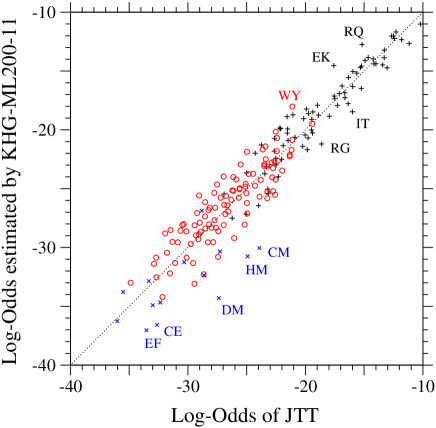
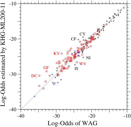
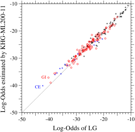
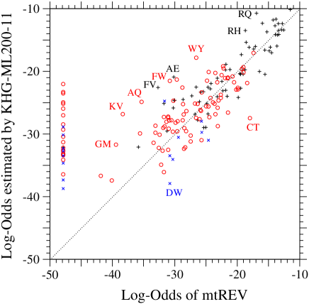
C                                                                                                                                                D

Figure 4: The KHG-ML200-11 model fitted to each of JTT, WAG, LG, and mtREV. Each element log-$O(\langle S\rangle(\hat{\tau},\hat{\sigma}))_{ab}$ of the log-odds matrices of the KHG-ML200-11 model fitted to the 1-PAM matrices of (A) JTT, (B) WAG, (C) LG, and (D) mtREV is plotted against the log-odds log-$O(S^{{\mbox{\scriptsize LG}}}(\mbox{1 PAM}))_{ab}$ calculated from the corresponding empirical substitution matrices. Plus, circle, and cross marks show the log-odds values for one-, two-, and three-step amino acid pairs, respectively. The dotted line in each figure shows the line of equal values between the ordinate and the abscissa. The log-odds elements of mtREV whose values are smaller than about $-47.8$ are all assumed to be $-47.8$; see the original paper [6].

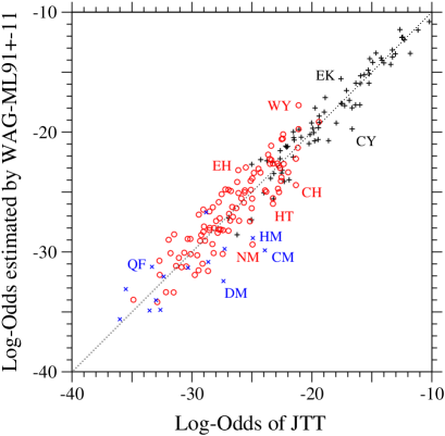
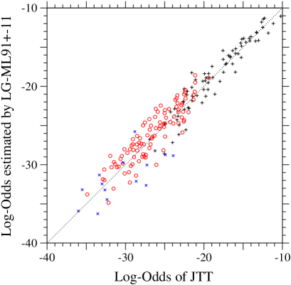
C                                                                                                                                          D

     

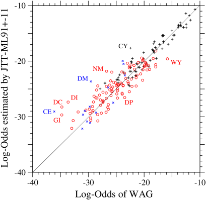
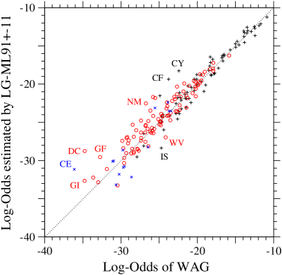
E                                                                                                                                          F

     

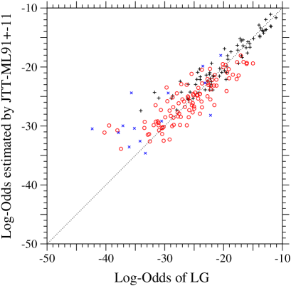
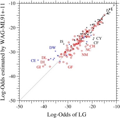
Figure S5: Models fitted to each of JTT, WAG, and LG. Each element log-$O(\langle S\rangle(\hat{\tau},\hat{\sigma}))_{ab}$ of the log-odds matrix of the model fitted to each empirical substitution matrix is plotted against the log-odds log-$O(S^{{\mbox{\scriptsize obs}}}(\mbox{1 PAM}))_{ab}$ calculated from the corresponding empirical substitution matrix. Plus, circle, and cross marks show the log-odds values for one-, two-, and three-step amino acid pairs, respectively. The dotted line in each figure shows the line of equal values between the ordinate and the abscissa.

The log-odds values of amino acid pairs estimated by the KHG-ML200-11 are plotted against their empirical values for the 1-PAM amino acid substitution matrices of JTT, WAG, LG, and mtREV in Fig. 4. Similar plots are shown in Figs. S5 – S10. The comparisons of Fig. 1 and Fig. S1 for the ML-87 model with Fig. 4 and Fig. S5 clearly indicate the good qualities of the ML estimators $\hat{w}_{ab}^{{\mbox{\scriptsize KHG-ML200}}}$ and $\hat{w}_{ab}^{{\mbox{\scriptsize JTT/WAG/LG-ML91+}}}$. Relatively large disagreements between empirical and estimated log-odds exist for cpREV and mtREV in comparison with those for JTT, WAG, LG, and the KHG-derived amino acid substitution matrix (KHGaa); see Fig. 4 and Figs. S5 – S7. It is unknown whether the disagreements shown in these figures represent meaningful features in the amino acid substitutions in the chloroplast DNA and the mitochondrial DNA or result from the relatively small size of sequence data used for cpREV and mtREV. However, the large disagreements in the region of low log-odds values may be artifacts, because cpREV and mtREV tend to include relatively large errors in this region, especially for mtREV; the log-odds values for mtREV whose values are smaller than about $-47.8$ are all assumed to be $-47.8$; see the original paper [6].

The ML estimates of $1/\beta$ listed in Tables 6, 7, and 8 indicate that the strength of selective constraints on amino acids is strong in the order of LG, WAG, and JTT. The strength of selective constraints is also shown by the change of the ratio of nonsynonymous to synonymous rate per codon between the two cases without and with selective constraints, i.e., the cases of $w_{ab}=0$ and $\sigma\rightarrow 0$, and $\sigma\rightarrow 0$. As already noted, the ratio of these values between the two cases represents the strength of selective constraints. In the KHG-ML200-11, these ratios are equal to $0.293/5.23=0.056$, $0.577/5.35=0.11$, and $0.499/3.71=0.13$ for LG, WAG, and JTT, respectively, meaning that the selective constraints of LG are strongest; it should be noted that this order agrees with the increasing order of $1/\hat{\beta}$.

Tables 6 and 7 indicate that the selective constraints $\hat{w}^{{\mbox{\scriptsize KHG-ML200}}}$ estimated from the KHG codon substitution matrix tend to estimate the contribution of multiple nucleotide changes ($m_{[tc][ag]}$) to be smaller, the ratio of transition to transversion exchangeability ($m_{tc|ag}/m_{[tc][ag]}$) to be smaller, $m_{ta}/m_{[tc][ag]}$ to be larger, and variations in substitution rates ($\sigma$) to be less than the $\hat{w}^{{\mbox{\scriptsize JTT/WAG/LG-ML91+}}}$ from the amino acid substitution matrices. Table 8 shows that the same characteristic differences will be observed if the JTT/WAG/LG-ML91+-11 models are fitted to the codon substitution matrix of KHG instead of its derived amino acid substitution matrix. Tables 6, 7, and 8 also show that the ratio of transition to transversion exchangeability ($m_{tc|ag}/m_{[tc][ag]}$) tends to be estimated to be smaller in the order of the LG-ML91+, the WAG-ML91+, the JTT-ML91+, and the KHG-ML200. The $m_{tc|ag}/m_{[tc][ag]}$ is estimated by the ML-91 or the ML-200 model to be smaller in the order of LG, WAG, JTT, and KHG; see Table 3. The present ML estimates $\{\hat{w}_{ab}\}$ for selective constraints on amino acids seem to reflect the characteristics of respective substitution matrices to which the models are fitted. It remains to be analyzed which estimation is better among the JTT/WAG/LG-ML91+ and the KHG-ML200 and how better it is. Irrespective of which estimation of the selection constraints is better, the ML estimates $\hat{m}_{tc|ag}/\hat{m}_{[tc][ag]}$ indicate that the transition to transversion bias is not so strong as previously estimated.

One of the interesting facts is that the ratio of the total transition to the total transversion rate per codon will be estimated to be much larger if multiple nucleotide changes are neglected; $\hat{m}_{tc|ag}/\hat{m}_{[tc][ag]}$ (and the ratio of the total transition to the total transversion rate for $\sigma\rightarrow 0$) are estimated for the mtREV to be 2.15 (3.32) in the JTT-ML91+-10 but 2.01 (2.52) in the JTT-ML91+-11, 4.27 (4.13) in the WAG-ML91+-10 but 3.43 (2.73) in the WAG-ML91+-11, 4.57 (4.74) in the LG-ML91+-10 but 3.82 (3.31) in the LG-ML91+-11, and 1.81 (2.58) in the KHG-ML200-10 but 1.64 (1.96) in the KHG-ML200-11. The same tendency is observed for JTT, WAG, cpREV, and mtREV irrespective of the matrices, and for the EI, the Miyata, and the Grantham models irrespective of the models.

In the case of mtREV, not only the transition-transversion exchangeability bias ($\hat{m}_{tc|ag}/\hat{m}_{[tc][ag]}$) but also the ratio of the total transition to the total transversion rate per codon is larger in the JTT/WAG/LG-ML91+-11 than in the JTT/WAG/LG-ML91+-0, and in the KHG-ML200-11 than in the KHG-ML200-0. Also, the JTT/WAG/LG-ML91+-11 and the KHG-ML200-11 models estimate $\hat{m}_{tc|ag}/\hat{m}_{[tc][ag]}$ and the ratio of the total transition to the total transversion rate to be larger for mtREV than for JTT, WAG, and cpREV. These results are consistent with a well-known fact that transition to transversion bias is larger in mitochondrial DNA than in nuclear DNA.

Discussion

Halpern and Bruno [40] considered a codon-substitution model in which site-specific selection is taken into account in terms of residue frequencies. If site-specific codon frequencies are explicitly taken into account in the present model, the substitution rate $R_{\mu\nu}$ will be regarded as the average of the site-specific rate $R^{i}_{\mu\nu}$ over sites $i$. According to Eq. 7, the site-specific rate is defined as the product of site-independent mutation rate $M_{\mu\nu}$ and site-dependent fixation probability, $(f^{i}_{\nu}/f^{{\mbox{\scriptsize mut}}}_{\nu})e^{w^{*}_{\mu\nu}}$.

$$R^{i}_{\mu\nu} = C_{{\mbox{\scriptsize onst}}}M_{\mu\nu}\frac{f^{i}_{\nu}}{f^{{\mbox{\scriptsize mut}}}_{\nu}}e^{w^{*}_{\mu\nu}}\;\mbox{ for }\mu\neq\nu$$ (32)

Here the site-dependency of the fixation probability is taken into account only in terms of codon frequencies. Then, the average of the site-specific rate over sites is calculated as follows.

$$R_{\mu\nu} \equiv C_{{\mbox{\scriptsize onst}}}\frac{\sum_{i}f^{i}_{\mu}R^{i}_{\mu\nu}}{\sum_{i}f^{i}_{\mu}}=C_{{\mbox{\scriptsize onst}}}M_{\mu\nu}\frac{f_{\nu}}{f^{{\mbox{\scriptsize mut}}}_{\nu}}e^{w_{\mu\nu}}\;\mbox{ for }\mu\neq\nu$$ (33)

$$e^{w_{\mu\nu}} \equiv e^{w^{*}_{\mu\nu}}\frac{\sum_{i}f^{i}_{\mu}f^{i}_{\nu}\sum_{j}1}{\sum_{i}f^{i}_{\mu}\sum_{j}f^{j}_{\nu}}$$ (34)

where $f_{\nu}$ is the average of $f^{i}_{\nu}$ over sites. Thus, the $w_{\mu\nu}$ defined here includes the effects of site-specific selection in terms of codon frequencies.

In the model of Halpern and Bruno [40], the term of $e^{w^{*}_{\mu\nu}}$ was not distinguished from and merged with the mutation rate $M_{\mu\nu}$; that is, $e^{w^{*}_{\mu\nu}}=\mbox{constant}$ for $\mu\neq\nu$ was assumed, Yang and Nielsen [22] considered mutation-selection models of codon substitutions and estimated selective strengths on codon usage. In their models, selection pressures that deviate codon frequencies from the equilibrium codon frequencies at the mutational level were explicitly taken into account, and selective constraints on amino acids are assumed to be constant over amino acid pairs; that is, $e^{w_{ab}}=\mbox{constant}$ for $a\neq b$ was assumed. However, the site-specific selection was not considered; that is, $f_{\mu}^{i}=f_{\mu}$. In other words, unlike the present model, selection was taken into account principally in terms of codon or residue frequencies in both the models. Also. multiple nucleotide changes were not taken into account. Halpern and Bruno [40] developed their model for distance calculation. As pointed out by Yang and Nielsen [22], taking account of site-specific codon frequencies is not practical for real data analysis due to the use of too many parameters. Instead, the use of $w_{\mu\nu}$ is more practical. The present results show that the ML values of the JTT/WAG/cpREV/mtREV amino acid substitution matrices are too small in the No-Constraints models in which $w_{ab}=0$ is assumed, and they can be improved by taking account of the term of the selective constraints $e^{w_{\mu\nu}}$. Also, it is indicated that selective constraints on amino acids strongly depend on the type of amino acid.

In some previous models [17, 18, 7], amino acid substitutions were assumed to proceed in a stepwise manner by successive single nucleotide changes in a codon. The empirical amino acid substitution matrices of JTT, WAG, LG, cpREV, and mtREV, and the codon substitution matrix KHG all include many substitutions between amino acid or codon pairs requiring multiple nucleotide changes. Significance of multiple nucleotide substitutions was pointed out [7, 20, 27, 29, 14]. There are two possible mechanisms to yield substitutions between such multi-step amino acid pairs even for a short time interval. One is variations in substitution rates or time intervals. Another is multiple nucleotide changes in a codon. Here, the assumption of multiple nucleotide changes has been directly introduced into a codon-based substitution model together with the use of a $\Gamma$ distribution for variations in substitution rates and time intervals, and the effectiveness of the assumption has been examined.

In the models using any physico-chemical evaluation of selective constraints, the significance of multiple nucleotide changes has been indicated; see Tables 2 and 3. The ML-87 models fitted to JTT and WAG, in which the selective constraints $\{w_{ab}\}$ for all single-step amino acid pairs are optimized by maximizing the likelihood with the assumptions of no multiple nucleotide change for codon substitutions and of variations in substitution rates, reveal that large discrepancies between the observed and the estimated log-odds values remain for multi-step amino acid pairs; see Fig. 1. When multiple nucleotide changes are taken into account in the model ML-91, these discrepancies disappear and the AIC values significantly decrease, indicating the significance of multiple nucleotide changes in codon substitutions; see Fig. 1, Fig. S1, and Table 3.

Evidence for multiple nucleotide changes was found by Averof et al. [27], and the frequency of multiple nucleotide changes was evaluated [20]. On the other hand, a possibility for successive single compensatory substitutions was pointed out by Bazykin et al. [29]. As pointed out by Kosiol et al. [14], the high exchangeabilities of the double nucleotide changes, Rcgt $\leftrightarrow$ Ragg and Rcgt $\leftrightarrow$ Raga, in KHG may result from successive single compensatory substitutions. On the other hand, a selection on synonymous substitutions is necessary for compensatory substitutions to cause the higher exchangeability of Rcga $\leftrightarrow$ Ragg than estimated, because the most probable paths of single nucleotide changes between Rcga and Ragg are Rcga $\leftrightarrow$ Raga $\leftrightarrow$ Ragg and Rcga $\leftrightarrow$ Rcgg $\leftrightarrow$ Ragg both of which do not accompany any amino acid change; see Fig. 2. Whatever causes multiple nucleotide changes, the present scheme for codon substitutions could be applied to phylogenetic analyses of protein-coding sequences, because the underlying time scale in the present substitution model is much longer than that of positive selection for successive single compensatory substitutions.

The models JTT/WAG/LG-ML91+-0 and KHG-ML200-0, in which parameters are taken to be equal to the ML estimates for JTT/WAG/LG in the ML-91+ model and the ML estimates for KHG in the ML-200 model, are codon-based models corresponding to the JTT/WAG/LG/KHG-F model, respectively. The model ML-91+ can almost perfectly reproduce JTT, WAG, and LG. The model ML-200 for the KHG codon substitution matrix can well reproduce the codon substitution probabilities for the codon pairs for which any nucleotide change is accompanied by an amino acid change, although the exchangeabilities of the other codon pairs are over-estimated for KHG. This means that the JTT/WAG/LG-ML91+-0 and the KHG-ML200-0 models can be used as a simple substitution model without any loss of information instead of the empirical substitution matrices of the JTT/WAG/LG/KHG in maximum likelihood and Bayesian inferences of phylogenetic trees of amino acid and codon sequences, respectively. Although the empirical substitution matrices represent the average tendencies of substitutions over proteins and species and may lack gene-level resolution [15, 16], the present mechanistic codon model has adjustable parameters for nucleotide mutation and for the strength of selective constraints, which can be tailored to specific genes. It is possible to optimize the selective constraints $\{w_{ab}\}$ for each gene. However, such a method [12, 15, 16] is far more computer-intensive than the present method. The present methods, JTT/WAG/LG-ML91+-$n$ using $\hat{w}^{{\mbox{\scriptsize JTT/WAG/LG-ML91+}}}$ and the KHG-ML200-$n$ with the $\hat{w}^{{\mbox{\scriptsize KHG-ML200}}}$, provide alternative models for amino acid/codon substitutions with a small number of ML parameters in the probabilistic inference of phylogenetic trees. The number of ML parameters specific to the present model is at most 6 exchangeabilities and 3 equilibrium frequencies for nucleotide mutations, and 2 parameters for selective constraints. Thus, the present model requires the same order of cpu time as the nucleotide substitution model (GTR) does. In other codon models [21, 23], exchangeabilities between amino acids are taken to be equal to their values in empirical amino acid substitution matrices. However, in the present codon model, amino acid and codon exchangeabilities vary according to nucleotide mutation rates and the strength of selective constraints.

The parameters $m_{\xi\eta}$, $f_{\xi}$, and $\sigma$ are differently estimated by the KHG-ML200-$n$ and the JTT/WAG/LG-ML91+-$n$ using different $\hat{w}$; see Tables 6, 7, and 8. The $\hat{w}^{{\mbox{\scriptsize KHG-ML200}}}$ yields a smaller rate of multiple nucleotide changes, a smaller $\sigma$, a smaller ratio of transition to transversion exchangeability, and a smaller ratio of nonsynonymous to synonymous rate per codon than the $\hat{w}^{{\mbox{\scriptsize JTT/WAG/LG-ML91+}}}$ does. Whichever estimation is better, the present ML estimators $\hat{m}_{tc|ag}/\hat{m}_{[tc][ag]}$ for transition-transversion bias strongly indicate that the transition-transversion bias is not so large as previously estimated. An excess of transitional over transversional substitutions was shown in the DNA sequences of metazoa, and has been assumed to be universal. However, Keller et al. [41] found a counter example to the transition-transversion bias from grasshopper pseudogenes. The present ML estimate of the ratio of transition to transversion exchangeability for the KHG codon substitution matrix is rather less than 1.0, i.e., $\hat{m}_{tc|ag}/\hat{m}_{[tc][ag]}=0.843$ in the ML-200 model, which corresponds to the overall rate bias of transitions over transversions, $0.427$. Even for the amino acid substitution matrices JTT, WAG, and LG, the ML-91 model estimates $m_{tc|ag}/m_{[tc][ag]}$ to be less than $1.9$, making the overall rate bias of transitions over transversions less than $1.0$; see Table 3. It should be noted that the ratio of transition to transversion exchangeability tends to be overestimated if no multiple nucleotide change is allowed; see Tables S2 and S3. Thus, the present results indicate that transition-transversion bias is not a solid assumption. On the other hand, the present results indicate that transition-transversion bias is stronger in mitochondrial DNA than in nuclear DNA in accordance with previous understanding; see Tables 6 and 7.

The ML estimates $\{\hat{w}^{{\mbox{\scriptsize JTT/WAG/LG-ML91+}}}_{ab}\}$ and $\{\hat{w}^{{\mbox{\scriptsize KHG-ML200}}}_{ab}\}$ significantly correlate with each other and also with the mean energy increments due to an amino acid replacement. However, the JTT/WAG/LG-ML91+-$n$ and KHG-ML200-$n$ models fit substitution data significantly better than the EI-$n$ model; see Tables 2 and 5. This fact indicates that the differences between the physico-chemical estimates and the ML estimates $\{\hat{w}_{ab}\}$ for selective pressure at the amino acid level reflect the actual tendency of selective constraints for respective types of amino acid pairs in protein evolution. Eq. 34 indicates that the $w$ is modulated by site-specific codon frequencies and differentiated from the site-independent constraints, $w^{*}$, which may be more similar to the physico-chemical estimates than the $w$. The selective constraints estimated here may be used as a base line to detect evidence of positive selection. Models [20, 22] in which the dependences of selective constraints on amino acid pairs are not taken into account may be improved by introducing them. On the other hand, it still remains to be examined whether or not the JTT/WAG/LG-ML91+-$n$ and the KHG-ML200-$n$ perform comparably with cpREV for the maximum likelihood inferences of phylogenetic trees of chloroplast proteins and with mtREV for those of mitochondrial proteins. Also, it should be examined which performs better.

A preliminary calculation has been pursued to examine the performance of the present substitution models in the ML inference of a phylogenetic tree. Log-likelihoods of the present models and the codon models corresponding to the mtREV-F, the JTT-F, the WAG-F, and the LG-F are calculated and listed in Table 9 for a phylogenetic tree [6] of the concatenated sequences of 12 protein-coding sequences encoded on the same strand of mitochondrial DNA from 20 vertebrate species with 2 races from human. The phylogenetic tree and the proteins used are those which Adachi and Hasegawa [6] used to estimate mtREV; the Japanese mtDNA was not used because it couldn’t be found in the GenBank database. The coding sequences of each protein were aligned with codon score matrices by the ClustalW2 [42], and then concatenated. Their likelihoods on the phylogenetic tree were calculated by the Phyml [43]. Both the programs have been modified for the analysis of coding sequences. Log-odds calculated by the KHG-ML200-11 fitted to mtREV were used as the codon score matrices. Positions with gaps are included for the calculation of the likelihoods. The codon substitution matrices corresponding to mtREV, JTT, WAG, LG, and the KHG-derived amino acid substitution matrix (KHGaa) are calculated in such a way that codon exchangeabilities for nonsynonymous codon pairs are taken to be equal to $\exp w_{0}$ multiplied by the exchangeability of the corresponding amino acid pair and those for synonymous codon pairs are assumed to be all equal to the mean amino acid exchangeability. In all models, the parameter $w_{0}$ in Eq. 14 was optimized even for the No-Constraints models, and codon frequencies were taken to be equal to those in coding sequences. The substitution matrices, JTT, WAG, LG, and KHG were estimated from nuclear DNA, which use a different genetic code from vertebrate mtDNA. On the other hand, mtREV was estimated by a maximum likelihood method from the almost same set of the protein sequences encoded in mtDNA. Thus, it is expected that the log-likelihood values of the mtDNA phylogenetic tree for the models, KHGaa-1-F, LG-1-F, WAG-1F, and JTT-1-F are worse than that for the mtREV-1-F. An important thing is that the codon models with the selective constraints estimated from nuclear DNA or by the physico-chemical method yield a much smaller value of AIC than the mtREV-1-F. One of the effective parameters is $w_{0}$ that directly controls the ratio of nonsynonymous to synonymous substitution rate. It also improves the likelihood to explicitly take account of rate variations over sites. The discrete approximation [44] of the $\Gamma$ distribution with 4 categories was used to represent rate variations over sites in the models named with the suffix ”dG4”; the shape parameter $\alpha$ is a ML parameter. An interesting and reasonable fact is that averaging substitution matrices over rate becomes unnecessary, i.e., $\hat{\sigma}=0.0$, in the case that rate variations over sites are explicitly taken into account; in the Yang’s model [26, 44], the likelihood of a phylogenetic tree of each site is averaged over rate. Also, all the present codon-based models estimate $\hat{m}_{[tc][ag]}>0.1$, which indicates the significance of multiple nucleotide changes. The present results strongly indicate that the tendencies of nucleotide mutations and codon usage are characteristic of a genetic system specific to each species and oranelle, but the amino acid dependences of selective constraints are more specifc to each type of amino acid than each species, organelle, and protein family. Full evaluation will be provided in a succeeding paper.

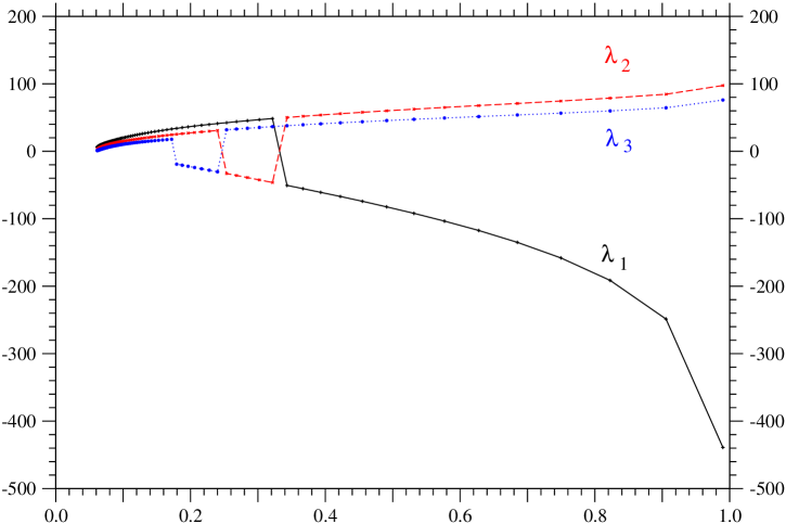
B

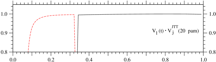
C

D

Figure S11: Temporal changes of the eigenvalues and the eigenvectors of the log-odds matrix log-$O(\langle S\rangle(t))$ calculated by the ML-91+ model fitted to JTT as a function of sequence identity. In (A), the solid, the broken, and the dotted lines show the temporal changes of the first ($\lambda_{1}$), the second ($\lambda_{2}$), and the third ($\lambda_{3}$) principal eigenvalues, respectively. The inner products of the eigenvectors with the eigenvectors of the JTT 20-PAM log-odds matrix, $\mbox{\boldmath{$V$}}_{i}(t)\cdot\mbox{\boldmath{$V$}}_{j}^{{\mbox{\scriptsize JTT}}}(\mbox{20-PAM})$, are shown in (B) for the first principal eigenvector ($i=1$), in (C) for the second principal eigenvector ($i=2$), and in (D) for the third principal eigenvector ($i=3$), by solid lines for $j=1$, by broken lines for $j=2$, and by dotted lines for $j=3$.

One may question whether the whole evolutionary process of protein-coding sequences can be approximated by a reversible Markov process or not. Kinjo and Nishikawa [45] reported that the log-odds matrices constructed for 18 different levels of sequence identities from structure-based protein alignments have a characteristic dependence on time in the principal components of their eigenspectra. Although they did not explicitly mention, this type of temporal process peculiar to the log-odd matrix in protein evolution is fully encoded in the transition matrices of JTT, WAG, LG, and KHG. In Fig. S11, it is shown that this characteristic dependence of log-odds on time can be reproduced by the transition matrix based on the present reversible Markov model fitted to JTT; see Supporting Information, Text S1, for details. This fact supports the appropriateness of the present Markov model for codon substitutions. The present codon-based model can be used to generate log-odds for codon substitutions as well as amino acid substitutions. Such a log-odds matrix of codon substitutions would be useful to allow us to align nucleotide sequences at the codon level rather than the amino acid level, increasing the quality of sequence alignments.

As a result, the present model would enable us to obtain more biologically meaningful information at both nucleotide and amino acid levels from codon sequences and even from protein sequences, because this is a codon-based model.

A                                                                                                                                                B

     

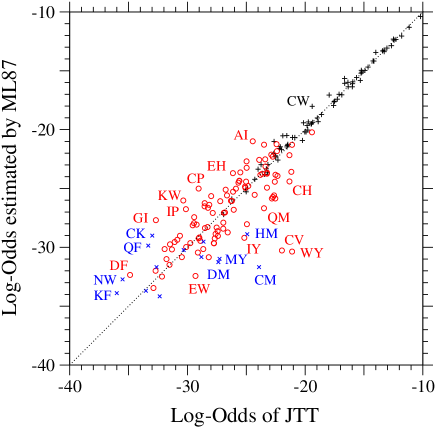
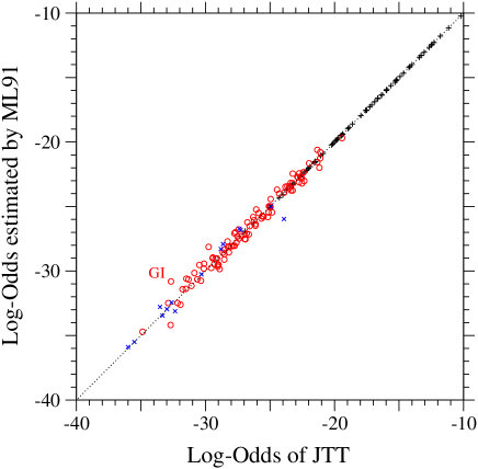
Figure 1: The ML-87 and the ML-91 models fitted to JTT. Each element log-$O(\langle S\rangle(\hat{\tau},\hat{\sigma}))_{ab}$ of the log-odds matrices of (A) the ML-87 and (B) the ML-91 models fitted to the 1-PAM JTT matrix is plotted against the log-odds log-$O(S^{{\mbox{\scriptsize JTT}}}(\mbox{1 PAM}))_{ab}$ calculated from JTT. Plus, circle, and cross marks show the log-odds values for the types of substitutions requiring single, double and triple nucleotide changes, respectively. The dotted line in each figure shows the line of equal values between the ordinate and the abscissa.

A                                                                                                                                                B

     

     

A                                                                                                                                                B

     

A                                                                                                                                                B

     

     

Table 1: Brief description of models.

Model name	Description
No-Constraints-$n$	No amino acid dependences of selective constraints; $\beta=0$. The suffix $n$ means the number of ML parameters.
EI-$n$	$\hat{w}_{ab}^{{\mbox{\scriptsize estimate}}}\equiv\Delta\hat{\varepsilon}^{{\mbox{\scriptsize c}}}_{ab}+\Delta\hat{\varepsilon}^{{\mbox{\scriptsize v}}}_{ab}$ based on the Energy-Increment-based (EI) method, which is described in Supporting Information, Text S1, is used to estimate $w_{ab}$ in Eq. 14. The suffix $n$ means the number of ML parameters.
Miyata-$n$	The amino acid pair distance $d_{ab}$ estimated by Miyata et al. [32] is used as $w_{ab}^{{\mbox{\scriptsize estimate}}}=-d_{ab}$ to estimate $w_{ab}$ in Eq. 14. The suffix $n$ means the number of ML parameters.
Grantham-$n$	The amino acid distance $d_{ab}$ estimated by Grantham [31] is used as $w_{ab}^{{\mbox{\scriptsize estimate}}}=-d_{ab}$ to estimate $w_{ab}$ in Eq. 14. The suffix $n$ means the number of ML parameters.
ML-$n$	Selective constraints $\{w_{ab}\}$ are estimated by maximizing the likelihood of JTT [5], WAG [10], or LG [11], and called $\{w_{ab}^{{\mbox{\scriptsize JTT/WAG/LG-ML}}n}\}$. The suffix $n$ means the number of ML parameters. In the ML-87, multiple nucleotide changes are disallowed, and $\{w_{ab}\}$ for all 75 single-step amino acid pairs are estimated. In the ML-91 and the ML-94, multiple nucleotide changes are allowed, and $\{w_{ab}\}$ for all 75 single-step amino acid pairs and for 6 groups of multiple-step amino acid pairs are estimated. In the ML-91, equal codon usage is assumed. In the ML-200 for codon substitution matrices, $\{w_{ab}\}$ for all 190 amino acid pairs are estimated.
ML-$n+$	First, the ML-$n$ is used to estimate parameters, and then $\{w_{ab}\}$ for all multiple-step amino acid pairs are estimated by maximizing the likelihood with fixing all other parameters to the values estimated by the ML-$n$.
JTT-ML91-$n$, WAG-ML91-$n$, LG-ML91-$n$	Selective constraints $\{w_{ab}^{{\mbox{\scriptsize JTT/WAG/LG-ML91}}}\}$ estimated by maximizing the likelihood of JTT/WAG/LG [5, 10, 11] in the ML-91 model are used as $\{w_{ab}^{{\mbox{\scriptsize estimate}}}\}$ in Eq. 14. The suffix $n$ means the number of ML parameters.
JTT-ML91+-$n$, WAG-ML91+-$n$, LG-ML91+-$n$	Selective constraints $\{w_{ab}^{{\mbox{\scriptsize JTT/WAG/LG-ML91+}}}\}$ estimated by maximizing the likelihood of JTT/WAG/LG [5, 10, 11] in the ML-91+ model are used as $\{w_{ab}^{{\mbox{\scriptsize estimate}}}\}$ in Eq. 14. The suffix $n$ means the number of ML parameters. The JTT/WAG/ LG-ML91+-0 models correspond to the JTT/WAG/LG-F models, respectively.
KHG-ML200-$n$	Selective constraints $\{w_{ab}^{{\mbox{\scriptsize KHG-ML200}}}\}$ estimated by maximizing the likelihood of the KHG codon substitution matrix [14] in the ML-200 model are used as $\{w_{ab}^{{\mbox{\scriptsize estimate}}}\}$ in Eq. 14. The suffix $n$ means the number of ML parameters. The KHG-ML200-0 models correspond to the KHG-F model.

Table 2: $\Delta$AIC values of the present models without and with the selective constraints on amino acids, which are based on mean energy increments due to an amino acid substitution (EI), the Miyata’s and the Grantham’s physico-chemical distances, for the 1-PAM amino acid substitution matrices of JTT, WAG, cpREV, and mtREV.

		$\Delta\mbox{AIC}\ ^{a}$
Model	#parameters	JTT	WAG	cpREV	mtREV
	(id no. b)
No-Constraints-
1	21($\beta=0$, 3)	86428.1	37917.6	3478.0	2644.1
10	30($\beta=0$, 2-10,14)	24595.6	7719.1	904.5	901.0
13	33($\beta=0$, 2-14)	22913.6	7141.5	874.9	798.8
EI-
2	22(1,3)	77337.9	35058.8	3186.0	2396.6
2G	22(1,14)	24197.7	5571.6	974.0	1066.8
3	23(1,3,14)	16463.7	4995.0	761.5	776.4
4	24(1-3,14)	15808.7	4443.6	743.0	753.9
8	28(1-7,14)	15715.0	4327.8	722.0	728.2
7	27(1-3,8-10,14)	15081.0	4312.6	650.7	688.7
10	30(1,3-10,14)	15435.7	4801.8	670.7	702.8
10M	30(1-10)	15270.7	4250.4	645.3	674.3
11	31(1-10,14)	14999.0	4202.5	636.0	674.3
10MU	30(1-3,8-14)	13464.3	3959.7	578.9	662.4
12	32(1,3-13)	72316.3	33908.4	2939.7	2215.0
13	33(1,3-14)	13819.7	4554.2	623.6	655.5
13M	33(1-13)	13436.2	3822.4	551.1	623.3
14	34(1-14)	13151.9	3748.0	541.9	614.8
Miyata-
4	24(1-3,14)	16090.1	4938.1	750.3	783.0
7	27(1-3,8-10,14)	15767.2	4715.4	654.5	701.6
10	30(1,3-10,14)	16446.1	5124.9	679.2	708.5
11	31(1-10,14)	15536.8	4429.5	628.4	658.4
13	33(1,3-14)	15058.2	4943.1	656.5	682.3
14	34(1-14)	14338.5	4254.0	603.7	613.6
Grantham-
4	24(1-3,14)	20505.1	5953.7	916.4	887.1
7	27(1-3,8-10,14)	18898.2	5814.0	840.6	832.9
10	30(1,3-10,14)	18744.5	5749.0	805.4	799.8
11	31(1-10,14)	18680.9	5579.7	803.2	796.5
13	33(1,3-14)	16784.9	5512.9	765.0	741.0
14	34(1-14)	16729.7	5477.1	755.0	739.5

^a $\Delta\mbox{AIC}\equiv 2N\hat{I}_{KL}(\hat{\mbox{\boldmath{$\theta$}}})+2\times$ #parameters with $N\simeq 5919000$ for JTT, $N\approx 1637663$ for WAG, $N\approx 169269$ for cpREV, and $N\approx 137637$ for mtREV; see text for details.

^b ML parameters in each model are specified by the parameter id numbers in the parenthesis, and other parameters are fixed at $\mbox{id}_{0}=0$, $\mbox{id}_{1}=\infty$, $\mbox{id}_{2}\rightarrow 0$, $\mbox{id}_{3-7}=1.0$, $\mbox{id}_{8-13}=0.5$, and $\mbox{id}_{14}\rightarrow 0$. Each id number corresponds to the parameter id number listed in Table 3.

Table 3: ML estimates and $\Delta$AIC values of the present models for the 1-PAM amino acid substitution matrices of JTT, WAG, and LG, and the 1-PAM codon substitution matrix of KHG.

		JTT			WAG			LG		KHG
										(codon)
id	parameter	ML–87a	ML–91a	ML–94	ML–87a	ML–91a	ML–94	ML–91a	ML–94	ML–200
no.
0	$-\hat{w}_{0}$	N/A	N/A	N/A	N/A	N/A	N/A	N/A	N/A	N/A
1	$1/\hat{\beta}$	N/A	N/A	N/A	N/A	N/A	N/A	N/A	N/A	N/A
2	$\hat{m}_{[tc][ag]}$	($\rightarrow 0$)	0.637	0.662	($\rightarrow 0$)	1.28	1.29	1.08	1.19	0.939
3	$\hat{m}_{tc|ag}/\hat{m}_{[tc][ag]}$	0.0919	1.57	1.59	0.746	1.70	1.69	1.85	1.81	0.843
4	$\hat{m}_{ag}/\hat{m}_{tc|ag}$	1.77	1.14	1.15	1.98	1.32	1.31	1.23	1.21	0.945
5	$\hat{m}_{ta}/\hat{m}_{[tc][ag]}$	0.0293	0.729	0.730	0.0477	0.791	0.784	0.676	0.682	1.52
6	$\hat{m}_{tg}/\hat{m}_{[tc][ag]}$	3.21	0.940	0.950	3.64	1.04	1.01	1.07	1.07	0.554
7	$\hat{m}_{ca}/\hat{m}_{[tc][ag]}$	0.719	1.19	1.18	0.110	1.23	1.23	1.28	1.25	0.573
8	$\hat{f}^{{\mbox{\scriptsize mut}}}_{t+a}$	0.408	0.459	0.446	0.372	0.367	0.392	0.388	0.403	0.497
9	$\hat{f}^{{\mbox{\scriptsize mut}}}_{t}/\hat{f}^{{\mbox{\scriptsize mut}}}_{t+a}$	0.113	0.501	0.522	0.234	0.587	0.513	0.450	0.439	0.513
10	$\hat{f}^{{\mbox{\scriptsize mut}}}_{c}/\hat{f}^{{\mbox{\scriptsize mut}}}_{c+g}$	0.698	0.429	0.436	0.425	0.479	0.471	0.427	0.383	0.470
11	$\hat{f}^{{\mbox{\scriptsize usage}}}_{t+a}$	0.0682	(0.5)	0.483	0.0669	(0.5)	0.221	(0.5)	0.447	NA
12	$\hat{f}^{{\mbox{\scriptsize usage}}}_{t}/\hat{f}^{{\mbox{\scriptsize usage}}}_{t+a}$	0.461	(0.5)	0.491	0.330	(0.5)	0.429	(0.5)	0.555	NA
13	$\hat{f}^{{\mbox{\scriptsize usage}}}_{c}/\hat{f}^{{\mbox{\scriptsize usage}}}_{c+g}$	0.386	(0.5)	0.558	0.310	(0.5)	0.306	(0.5)	0.249	NA
14	$\hat{\sigma}$	27.3	0.738	0.740	43.3	0.905	0.840	0.415	0.395	$\rightarrow 0$
$\hat{\tau}\hat{\sigma}$		0.334	0.0243	0.0246	0.317	0.0223	0.0207	0.0246	0.0240	0.0240
#parameters		107	111	114	107	111	114	111	114	261
$\hat{I}_{KL}(\hat{\mbox{\boldmath{$\theta$}}})\times 10^{8}\ {}^{b}$		$15695$	638	$613$	$35319$	1903	$1438$	2771	2335	269946
$\Delta\mbox{AIC}\ ^{c}$		2072.0	297.5	300.6	1370.8	284.3	275.1	782.5	700.4	unknown
Ratio of substitution rates
per codon
the total base/codon		1.28	1.35	1.35	1.38	1.53	1.52	1.38	1.39	1.29
										(1.29)d
transition/transversion		0.464	1.08	1.08	0.482	0.932	0.806	1.18	1.20	0.764
										(0.765)d
nonsynonymous/synonymouse		1.13	1.37	1.34	1.57	2.07	2.40	1.05	1.20	0.726
										(0.723)d
Ratio of substitution rates
per codon for $\sigma\rightarrow 0$
total base/codon		1.0	1.22	1.22	1.0	1.38	1.40	1.31	1.33	1.29
transition/transversion		0.101	1.21	1.22	0.647	1.11	0.932	1.31	1.35	0.764
nonsynonymous/synonymouse		0.0644	1.04	1.02	0.138	1.50	1.79	0.853	0.889	0.726
Ratio of substitution rates per
codon for $w_{ab}=0$ and $\sigma\rightarrow 0$
total base/codon		1.0	1.45	1.46	1.0	1.72	1.74	1.67	1.71	1.51
transition/transversion		0.0605	0.829	0.831	0.499	0.933	0.849	0.992	0.981	0.427
nonsynonymous/synonymouse		11.3	5.58	5.74	11.1	8.68	11.1	7.45	8.46	6.81

^a If the value of a parameter is parenthesized, the parameter is not variable but fixed to the value specified.

^b $\hat{I}_{KL}(\hat{\mbox{\boldmath{$\theta$}}})=-(\ell(\hat{\mbox{\boldmath{$\theta$}}})/N+2.98607330)$ for JTT, $-(\ell(\hat{\mbox{\boldmath{$\theta$}}})/N+2.97444860)$ for WAG, $-(\ell(\hat{\mbox{\boldmath{$\theta$}}})/N+2.96853414)$ for LG, and $-(\ell(\hat{\mbox{\boldmath{$\theta$}}})/N+4.19073314)$ for KHG; see text for details.

^c $\Delta\mbox{AIC}\equiv 2N\hat{I}_{KL}(\hat{\mbox{\boldmath{$\theta$}}})+2\times$ #parameters with $N\simeq 5919000$ for JTT, $N\approx 1637663$ for WAG, $N\approx 10114373$ for LG, and the value of $N$ is unknown for KHG; see text for details.

^d The value in the parenthesis corresponds to the one for the KHG codon substitution probability matrix.

^e Note that these ratios are not the ratios of the rates per site but per codon; see text for details.

Table 4: Correlations of $\hat{w}_{ab}$ between various estimates; the lower half shows the correlation coefficients of $\hat{w}_{ab}$ for 75 single-step amino acid pairs and the upper half does those of $\hat{w}_{ab}$ for 86 multi-step amino acid pairs by excluding 29 amino acid pairs of the least exchangeable category in the JTT-ML91, the WAG-ML91 or the LG-ML91.

Model	EI	JTT-ML91+	WAG-ML91+	LG-ML91+	KHG-ML200
EI		0.45	0.51	0.59	0.55	(0.65)a
JTT-ML91+	0.66		0.80	0.80	0.51
WAG-ML91+	0.68	0.87		0.86	0.55
LG-ML91+	0.71	0.82	0.90		0.58
KHG-ML200	0.71	0.77	0.69	0.74

^a The value in the parenthesis is the correlation coefficient for which the $\hat{w}_{ab}$ for all multi-step amino acid pairs are taken into account. The correlation coefficient of $\hat{w}_{ab}$ for all amino acid pairs between the EI and the KHG-ML200 is equal to 0.60.

Table 5: $\Delta$AIC values of the present models with the respective selective constraints on amino acids, $\hat{w}^{{\mbox{\scriptsize JTT-ML91+}}}$, $\hat{w}^{{\mbox{\scriptsize WAG-ML91+}}}$, $\hat{w}^{{\mbox{\scriptsize LG-ML91+}}}$, and $\hat{w}^{{\mbox{\scriptsize KHG-M200}}}$, for the various 1-PAM substitution matrices.

	#parameters	$\Delta\mbox{AIC}\ ^{b}$					$\hat{I}_{KL}(\hat{\mbox{\boldmath{$\theta$}}})\times 10^{8}\ {}^{c}$
Model name	#parameters	JTT	WAG	LG	cpREV	mtREV	KHG	KHG
	(id no. a)						(amino acid)	(codon)
JTT-ML91+-
0	20		2657.5	20807.0	461.7	426.0
1	21(14)		2065.1	20382.6	433.9	424.4
4	24(1-3,14)		1773.7	16148.3	439.2	401.9
7	27(1-3,8-10,14)		1257.8	12330.2	303.4	295.5
11	31(1-10,14)		1152.9	12140.0	291.5	286.5	40931
12	32(0-10,14)							473668
WAG-ML91+-
0	20	9095.4		10537.3	316.2	535.1
1	21(14)	8928.9		9196.3	317.1	532.8
4	24(1-3,14)	6274.9		6354.9	281.4	414.0
7	27(1-3,8-10,14)	3658.3		5294.9	261.6	383.6
11	31(1-10,14)	3299.2		4813.3	259.1	365.1	12789
12	32(0-10,14)							496804
LG-ML91+-
0	20	13669.8	1806.0		487.1	593.4
1	21(14)	12176.2	1188.8		421.4	558.0
4	24(1-3,14)	6325.7	811.6		340.6	391.6
7	27(1-3,8-10,14)	3983.0	636.0		267.0	329.8
11	31(1-10,14)	3878.5	574.7		267.1	314.9	5732
12	32(0-10,14)							436557
KHG-ML200-
0	20	15063.5	953.4	12568.9	403.6	593.6
1	21(14)	15078.6	955.4	12570.9	405.6	595.6
4	24(1-3,14)	6398.0	540.7	5683.3	297.4	399.3
7	27(1-3,8-10,14)	4611.5	533.4	3804.2	259.9	358.0
11	31(1-10,14)	4429.9	518.7	3006.1	251.7	334.1

^a Parameter id numbers in the parenthesis mean ML parameters in each model and other parameters except for $\beta=1$ and $w_{0}=0$ are fixed to the value of the corresponding parameter listed in the column of the ML-91 or the ML-200 in Table 3; each id number corresponds to the parameter id number listed in Table 3.

^b $\Delta\mbox{AIC}\equiv 2N\hat{I}_{KL}(\hat{\mbox{\boldmath{$\theta$}}})+2\times$ #parameters with $N\simeq 5919000$ for JTT, $N\approx 1637663$ for WAG, $N\approx 10114373$ for LG, $N\approx 169269$ for cpREV, and $N\approx 137637$ for mtREV; see text for details.

^c $\hat{I}_{KL}(\hat{\mbox{\boldmath{$\theta$}}})=$ $-(\ell(\hat{\mbox{\boldmath{$\theta$}}})/N+2.97009788)$ for the KHG-derived amino acid substitution probability matrix, and $-(\ell(\hat{\mbox{\boldmath{$\theta$}}})/N+4.19073314)$ for the KHG codon substitution probability matrix; see text for details.

Table 6: ML estimates of the present models with the respective selective constraints for the 1-PAM amino acid substitution matrices of JTT, WAG, and LG.

	JTT			WAG			LG
	WAG- a	LG- a	KHG- a	JTT- a	LG- a	KHG- a	JTT- a	WAG- a	KHG- a
	ML91+-11		ML200-11	ML91+-11		ML200-11	ML91+-11		ML200-11
$-\hat{w}_{0}$	(0.0)	(0.0)	(0.0)	(0.0)	(0.0)	(0.0)	(0.0)	(0.0)	(0.0)
$1/\hat{\beta}$	1.08	1.32	1.07	1.04	1.28	1.01	0.830	0.798	0.757
$\hat{m}_{[tc][ag]}$	0.429	0.304	0.257	1.29	0.921	0.648	1.45	1.543	0.577
$\hat{m}_{tc|ag}/\hat{m}_{[tc][ag]}$	2.36	2.42	1.26	1.19	1.71	0.850	1.16	1.82	0.783
$\hat{m}_{ag}/\hat{m}_{tc|ag}$	1.22	1.16	0.915	1.26	1.27	1.00	1.20	1.26	0.869
$\hat{m}_{ta}/\hat{m}_{[tc][ag]}$	0.649	0.654	1.32	0.814	0.802	1.54	0.668	0.634	1.59
$\hat{m}_{tg}/\hat{m}_{[tc][ag]}$	1.13	1.01	0.622	0.862	0.947	0.568	0.988	1.20	0.524
$\hat{m}_{ca}/\hat{m}_{[tc][ag]}$	1.18	1.31	0.605	1.27	1.33	0.597	1.24	1.20	0.446
$\hat{f}^{{\mbox{\scriptsize mut}}}_{t+a}$	0.481	0.507	0.578	0.351	0.405	0.512	0.333	0.335	0.534
$\hat{f}^{{\mbox{\scriptsize mut}}}_{t}/\hat{f}^{{\mbox{\scriptsize mut}}}_{t+a}$	0.527	0.488	0.490	0.548	0.527	0.519	0.462	0.518	0.463
$\hat{f}^{{\mbox{\scriptsize mut}}}_{c}/\hat{f}^{{\mbox{\scriptsize mut}}}_{c+g}$	0.429	0.390	0.413	0.461	0.435	0.463	0.455	0.468	0.446
$\hat{\sigma}$	1.09	1.28	0.604	0.893	0.751	$\rightarrow 0$	0.886	0.718	$\rightarrow 0$
$\hat{\tau}\hat{\sigma}$	0.0263	0.0310	0.0363	0.0220	0.0230	0.0275	0.0246	0.0231	0.0444
#parameters	31	31	31	31	31	31	31	31	31
$\hat{I}_{KL}(\hat{\mbox{\boldmath{$\theta$}}})\times 10^{8}\ {}^{b}$	$27346$	$32239$	36897	$33306$	$15653$	13945	$59707$	$23488$	14554
$\Delta\mbox{AIC}\ ^{c}$	3299.2	3878.5	4429.9	1152.9	574.7	518.7	12140.0	4813.3	3006.1
Ratio of substitution
rates per codon
the total base/codon	1.35	1.32	1.19	1.51	1.45	1.19	1.47	1.49	1.12
transition/transversion	1.23	1.25	1.02	0.815	0.959	0.753	0.902	1.08	0.789
non-/synonymousd	1.49	1.17	0.612	2.07	1.59	0.577	1.56	1.60	0.293
For $\sigma\rightarrow 0$
the total base/codon	1.19	1.13	1.09	1.37	1.33	1.19	1.34	1.39	1.12
transition/transversion	1.51	1.57	1.06	0.923	1.10	0.753	1.03	1.29	0.789
non-/synonymousd	1.03	0.755	0.449	1.54	1.19	0.577	1.14	1.20	0.293
For $w_{ab}=0$ and $\sigma\rightarrow 0$
the total base/codon	1.38	1.29	1.18	1.66	1.60	1.38	1.68	1.80	1.34
transition/transversion	1.27	1.28	0.642	0.645	0.926	0.440	0.622	0.989	0.390
non-/synonymousd	4.67	3.99	3.71	8.62	7.02	5.35	8.79	9.49	5.23

^a In all models, equal codon usage ($\hat{f}^{{\mbox{\scriptsize usage}}}_{t}=\hat{f}^{{\mbox{\scriptsize usage}}}_{a}=\hat{f}^{{\mbox{\scriptsize usage}}}_{c}=\hat{f}^{{\mbox{\scriptsize usage}}}_{g}=0.25$) is assumed. If the value of a parameter is parenthesized, the parameter is not variable but fixed to the value specified.

^b $\hat{I}_{KL}(\hat{\mbox{\boldmath{$\theta$}}})=$ $-(\ell(\hat{\mbox{\boldmath{$\theta$}}})/N+2.98607330)$ for JTT, $-(\ell(\hat{\mbox{\boldmath{$\theta$}}})/N+2.97444860)$ for WAG, and $-(\ell(\hat{\mbox{\boldmath{$\theta$}}})/N+2.96853414)$ for LG.

^c $\Delta\mbox{AIC}\equiv 2N\hat{I}_{KL}(\hat{\mbox{\boldmath{$\theta$}}})+2\times$ #parameters with $N\simeq 5919000$ for JTT, $N\approx 1637663$ for WAG, and $N\approx 10114373$ for LG; see text for details.

^d Note that these ratios are not the ratios of the rates per site but per codon; see text for details.

Table 7: ML estimates of the present models with the respective selective constraints for the 1-PAM amino acid substitution matrices of cpREV and mtREV.

	cpREV				mtREV
	JTT- a	WAG- a	LG- a	KHG- a	JTT- a	WAG- a	LG- a	KHG- a
	ML91+-11			ML200-11	ML91+-11			ML200-11
$-\hat{w}_{0}$	(0.0)	(0.0)	(0.0)	(0.0)	(0.0)	(0.0)	(0.0)	(0.0)
$1/\hat{\beta}$	0.940	0.977	1.18	1.02	0.690	0.845	0.977	0.752
$\hat{m}_{[tc][ag]}$	0.865	0.917	0.611	0.521	0.564	0.524	0.321	0.228
$\hat{m}_{tc|ag}/\hat{m}_{[tc][ag]}$	1.50	2.23	2.353	1.14	2.01	3.43	3.82	1.64
$\hat{m}_{ag}/\hat{m}_{tc|ag}$	1.28	1.30	1.24	0.973	1.06	1.13	1.08	0.752
$\hat{m}_{ta}/\hat{m}_{[tc][ag]}$	0.746	0.705	0.733	1.61	0.681	0.595	0.638	2.00
$\hat{m}_{tg}/\hat{m}_{[tc][ag]}$	1.17	1.37	1.25	0.747	0.792	0.893	0.839	0.411
$\hat{m}_{ca}/\hat{m}_{[tc][ag]}$	1.23	1.17	1.26	0.566	1.65	1.67	1.76	0.623
$\hat{f}^{{\mbox{\scriptsize mut}}}_{t+a}$	0.283	0.306	0.328	0.442	0.262	0.270	0.287	0.426
$\hat{f}^{{\mbox{\scriptsize mut}}}_{t}/\hat{f}^{{\mbox{\scriptsize mut}}}_{t+a}$	0.611	0.654	0.609	0.597	0.601	0.652	0.598	0.631
$\hat{f}^{{\mbox{\scriptsize mut}}}_{c}/\hat{f}^{{\mbox{\scriptsize mut}}}_{c+g}$	0.425	0.446	0.393	0.425	0.349	0.304	0.260	0.332
$\hat{\sigma}$	1.93	1.43	1.75	0.158	3.48	2.18	3.37	2.89
$\hat{\tau}\hat{\sigma}$	0.0325	0.0285	0.0339	0.0288	0.0603	0.0445	0.0653	0.0923
#parameters	31	31	31	31	31	31	31	31
$\hat{I}_{KL}(\hat{\mbox{\boldmath{$\theta$}}})\times 10^{8}\ {}^{b}$	$67803$	$58229$	$60586$	56032	$81541$	$110126$	$91860$	98837
$\Delta\mbox{AIC}\ ^{c}$	291.5	259.1	267.1	251.7	286.5	365.1	314.9	334.1
Ratio of substitution
rates per codon
the total base/codon	1.45	1.46	1.41	1.20	1.36	1.37	1.33	1.23
transition/transversion	1.05	1.20	1.25	1.05	1.44	1.65	1.74	1.45
non-/synonymousd	1.74	1.80	1.38	0.631	0.908	1.04	0.772	0.403
For $\sigma\rightarrow 0$
the total base/codon	1.21	1.26	1.20	1.16	1.11	1.15	1.09	1.05
transition/transversion	1.42	1.66	1.77	1.07	2.52	2.73	3.31	1.96
non-/synonymousd	1.03	1.10	0.794	0.573	0.387	0.515	0.312	0.163
For $w_{ab}=0$ and $\sigma\rightarrow 0$
the total base/codon	1.45	1.55	1.44	1.33	1.31	1.37	1.26	1.16
transition/transversion	0.797	1.20	1.25	0.569	1.06	1.78	1.98	0.883
non-/synonymousd	6.06	6.33	5.14	4.97	3.40	3.09	2.58	3.02

^a In all models, equal codon usage ($\hat{f}^{{\mbox{\scriptsize usage}}}_{t}=\hat{f}^{{\mbox{\scriptsize usage}}}_{a}=\hat{f}^{{\mbox{\scriptsize usage}}}_{c}=\hat{f}^{{\mbox{\scriptsize usage}}}_{g}=0.25$) is assumed. If the value of a parameter is parenthesized, the parameter is not variable but fixed to the value specified.

^b $\hat{I}_{KL}(\hat{\mbox{\boldmath{$\theta$}}})=$ $-(\ell(\hat{\mbox{\boldmath{$\theta$}}})/N+2.95801048)$ for cpREV, and $-(\ell(\hat{\mbox{\boldmath{$\theta$}}})/N+2.85313622)$ for mtREV; see text for details.

^c $\Delta\mbox{AIC}\equiv 2N\hat{I}_{KL}(\hat{\mbox{\boldmath{$\theta$}}})+2\times$ #parameters with $N\approx 169269$ for cpREV, and $N\approx 137637$ for mtREV; see text for details.

^d Note that these ratios are not the ratios of the rates per site but per codon; see text for details.

Table 8: ML estimates of the present models with the respective selective constraints for the 1-PAM KHG-derived amino acid and KHG codon substitution matrices.

	KHG (amino acid)			KHG (codon)
	JTT- a	WAG- a	LG- a	JTT- a	WAG- a	LG- a
	ML91+-11			ML91+-12
$-\hat{w}_{0}$	(0.0)	(0.0)	(0.0)	1.29	1.50	1.11
$1/\hat{\beta}$	0.952	0.912	1.22	1.72	2.02	1.91
$\hat{m}_{[tc][ag]}$	1.545	1.68	1.33	1.23	1.21	1.15
$\hat{m}_{tc|ag}/\hat{m}_{[tc][ag]}$	1.19	1.73	1.69	0.992	1.07	1.09
$\hat{m}_{ag}/\hat{m}_{tc|ag}$	1.24	1.28	1.22	1.09	1.12	1.10
$\hat{m}_{ta}/\hat{m}_{[tc][ag]}$	0.689	0.682	0.748	1.26	1.25	1.25
$\hat{m}_{tg}/\hat{m}_{[tc][ag]}$	0.855	1.07	0.943	0.646	0.662	0.671
$\hat{m}_{ca}/\hat{m}_{[tc][ag]}$	1.32	1.26	1.31	0.815	0.806	0.813
$\hat{f}^{{\mbox{\scriptsize mut}}}_{t+a}$	0.317	0.334	0.377	0.480	0.484	0.488
$\hat{f}^{{\mbox{\scriptsize mut}}}_{t}/\hat{f}^{{\mbox{\scriptsize mut}}}_{t+a}$	0.533	0.579	0.512	0.499	0.499	0.493
$\hat{f}^{{\mbox{\scriptsize mut}}}_{c}/\hat{f}^{{\mbox{\scriptsize mut}}}_{c+g}$	0.460	0.480	0.441	0.464	0.459	0.459
$\hat{\sigma}$	2.64	2.25	1.30	$\rightarrow 0$	0.0496	$\rightarrow 0$
$\hat{\tau}\hat{\sigma}$	0.0308	0.0286	0.0247	0.0240	0.0247	0.0240
#parameters	31	31	31	32	32	32
$\hat{I}_{KL}(\hat{\mbox{\boldmath{$\theta$}}})\times 10^{8}\ {}^{b}$	40931	12789	5732	473668	496804	436557
Ratio of substitution
rates per codon
the total base/codon	1.64	1.66	1.59	1.29	1.29	1.29
transition/transversion	0.772	0.859	0.891	0.759	0.765	0.767
non-/synonymousc	2.56	2.61	2.03	0.728	0.727	0.724
For $\sigma\rightarrow 0$
the total base/codon	1.39	1.45	1.43	1.29	1.28	1.29
transition/transversion	0.977	1.15	1.08	0.759	0.770	0.767
non-/synonymousc	1.48	1.54	1.36	0.728	0.704	0.724
For $w_{ab}=0$ and $\sigma\rightarrow 0$
the total base/codon	1.71	1.83	1.75	1.65	1.65	1.64
transition/transversion	0.637	0.926	0.892	0.51	0.552	0.561
non-/synonymousc	9.41	10.3	8.86	8.16	8.07	7.77

^a In all models, codon frequencies are taken to be equal to the observed ones. If the value of a parameter is parenthesized, the parameter is not variable but fixed to the value specified.

^b $\hat{I}_{KL}(\hat{\mbox{\boldmath{$\theta$}}})=$ $-(\ell(\hat{\mbox{\boldmath{$\theta$}}})/N+2.97009788)$ for the KHG-derived amino acid substitution probability matrix, and $-(\ell(\hat{\mbox{\boldmath{$\theta$}}})/N+4.19073314)$ for the KHG codon substitution probability matrix; see text for details.

^d Note that these ratios are not the ratios of the rates per site but per codon; see text for details.

Table 9: Log-likelihoods of a phylogenetic tree [6] of the concatenated sequences of 12 protein-coding sequences encoded on the same strand of mitochondrial DNA from 20 vertebrate species with 2 races from human.

Codon Substitution	#pb	$\ell+$	$\mbox{AIC}-$	$\hat{\sigma}$	$\hat{m}_{[tc][ag]}$	$\hat{m}_{tc|ag}/\hat{m}_{[tc][ag]}$
Modela		$116898.6$	$233917.3$
LG-1-Fc	60	$-1293.8$	$2587.6$
KHGaa-1-Fcd	60	$-1293.0$	$2586.1$
WAG-1-Fc	60	$-1108.1$	$2216.1$
JTT-1-Fc	60	$-836.4$	$1672.8$
mtREV-1-Fc	60	$0.0$	$0.0$
No-Constraints-1-Fe	60	$-1731.0$	$3462.1$	$(2.46)$	$(0.040)$	$(3.24)$
WAG-ML91+-1-Fe	60	$1021.4$	$-2042.7$	$(2.18)$	$(0.524)$	$(3.43)$
JTT-ML91+-1-Fe	60	$1237.7$	$-2475.5$	$(3.48)$	$(0.564)$	$(2.01)$
LG-ML91+-1-Fe	60	$1382.2$	$-2764.4$	$(3.37)$	$(0.321)$	$(3.82)$
EI-1-Fe	60	$1395.8$	$-2791.6$	$(0.339)$	$(0.737)$	$(3.06)$
KHG-ML200-1-Fe	60	$1676.9$	$-3353.9$	$(2.89)$	$(0.228)$	$(1.64)$
No-Constraints-11-F	70	$772.2$	$-1524.4$	$0.906$	$0.273$	$3.37$
EI-12-F	71	$1966.6$	$-3911.2$	$0.326$	$0.549$	$3.60$
WAG-ML91+-12-F	71	$2268.3$	$-4514.5$	$1.84$	$0.471$	$4.16$
JTT-ML91+-12-F	71	$2275.1$	$-4528.1$	$3.57$	$0.506$	$2.91$
KHG-ML200-12-F	71	$2355.7$	$-4689.4$	$0.469$	$0.226$	$2.50$
LG-ML91+-12-F	71	$2510.0$	$-4997.9$	$1.26$	$0.357$	$4.32$
No-Constraints-11-F-dG4	71	$2495.4$	$-4968.9$	$0.000$	$0.182$	$3.62$
EI-12-F-dG4	72	$3742.4$	$-7460.7$	$0.000$	$0.392$	$3.95$
JTT-ML91+-12-F-dG4	72	$4156.9$	$-8289.8$	$0.064$	$0.385$	$3.11$
KHG-ML200-12-F-dG4	72	$4190.0$	$-8356.0$	$0.000$	$0.147$	$2.60$
WAG-ML91+-12-F-dG4	72	$4196.4$	$-8368.7$	$0.042$	$0.342$	$4.61$
LG-ML91+-12-F-dG4	72	$4412.6$	$-8801.1$	$0.029$	$0.253$	$4.83$

^a In all models named with a suffix ”F”, codon frequencies are taken to be equal to those in coding sequences. A suffix ”dG4” means the discrete approximation of the $\Gamma$ distribution with 4 categories [44] for rate variation. The parameter $w_{0}$ in Eq. 14 is optimized in all models.

^b The number of parameters; the value for the mtREV-1-F is not quite correct, because mtREV was estimated from the almost same set of protein sequences [6].

^c The exchangeabilties of nonsynonymous and synonymous codon pairs are equal to $\exp w_{0}$ multiplied by those of the corresponding amino acid pairs and all equal to the mean amino acid exchangeability in the empirical amino acid substitution matrix specified, respectively.

^d KHGaa means the amino acid substitution matrix derived from KHG.

^e All parameters except $w_{0}$ and codon frequencies are fixed to those ML estimates of each model fitted to mtREV.

Supporting Information Legends

Text S1. Supporting information consisting of the following sections.

1. A method for the physico-chemical evaluation of selective constraints on amino acid replacement.

2. Models with no amino acid dependences of selective constraints.

3. A physico-chemical evaluation of selective constraints on amino acids.

4. Other physico-chemical evaluations of selective constraints on amino acids.

5. Evolutionary process of amino acid substitutions in terms of log-odds.

Data S1. A computer-readable dataset of the ML estimates of parameters in the ML-200 for KHG, and the ML-91 and the ML-91+ for LG, WAG, and JTT as well as the EI.

Supporting Information
for
Selective Constraints on Amino Acids
Estimated by a Mechanistic Codon Substitution Model
with Multiple Nucleotide Changes

Sanzo Miyazawa

Graduate School of Engineering

Gunma University

Kiryu, Gunma 376-8515, Japan

Phone: +81-277-30-1940

E-Mail: miyazawa@smlab.sci.gunma-u.ac.jp

sanzo.miyazawa@gmail.com

()

Supplementary Methods

A method for the physico-chemical evaluation of selective constraints on amino acid replacements

Physico-chemical evaluations of $\{w_{ab}\}$ are not meaningless, even though selective constraints $\{w_{ab}\}$ in Eq. 12 in the text can be optimized for observed data. Their performance in reproducing observed substitution data indicates how extensively selective constraints on amino acid substitutions can be explained by physico-chemical requirements on amino acid substitutions to preserve protein structures and functions. In this section, a new physico-chemical method for the evaluation of the selective constraints is introduced.

The rate of acceptance in amino acid replacements is assumed here to be proportional to the mean relative stability of the native conformation $\mathcal{C}$ of the mutant type of sequence $\mathcal{S^{\prime}}$ to that of the wild type of sequence $\mathcal{S}$. The probability $P(\mathcal{C}|\mathcal{S})$ of a conformation $\mathcal{C}$ that a sequence $\mathcal{S}$ takes is equal to the Boltzmann factor of $\mathcal{C}$ divided by the conformational partition function of $\mathcal{S}$. The conformational partition function of a protein may be crudely approximated in the high temperature expansion.

$$\log P(\mathcal{C}|\mathcal{S})$$ (S1-1)

$$\simeq -\frac{1}{kT}\mathcal{E}(\mathcal{C},\mathcal{S})$$

$$\vspace*{1em}-[\log(\sum_{\mathcal{C}\in\{{\mbox{\scriptsize compact}}\}}1)-\frac{1}{kT}\langle\mathcal{E}(\mathcal{C},\mathcal{S})\rangle_{{\mbox{\scriptsize compact}},T\rightarrow\infty}]$$

where $k$ is the Boltzmann constant, $T$ is temperature, and $\mathcal{E}(\mathcal{C},\mathcal{S})$ is the conformational free energy of the conformation $\mathcal{C}$ taken by the sequence $\mathcal{S}$. First, the sum over conformations $\mathcal{C}$ are approximated by the sum over compact/nativelike conformations whose energies are significantly lower than those of extended conformations. Then, the logarithm of the partition function is approximated by the sum of the first and the second terms in the high temperature expansion. Thus, the relative stability of the native conformation of sequence $\mathcal{S^{\prime}}$ to that of sequence $\mathcal{S}$ is estimated by

$$\log[P(\mathcal{C}|\mathcal{S}^{\prime})/P(\mathcal{C}|\mathcal{S})]$$ (S1-2)

$$\simeq -\frac{1}{kT}(\mathcal{E}(\mathcal{C},\mathcal{S}^{\prime})-\mathcal{E}(\mathcal{C},\mathcal{S}))\mbox{ , }$$

if the amino acid composition does not change.

The mean energy of compact conformations does not depend on the details of the amino acid order in protein sequences but primarily on the amino acid composition. Therefore, if the amino acid composition keeps constant during amino acid substitutions, as indicated by the present assumption of the stationary state for amino acid substitutions, the relative stability can be approximated by the difference of the native conformational energies of the two sequences.

As a result, the parameter $w_{ab}$, whose exponent is the acceptance rate of substitutions between amino acids of type $a$ and type $b$, is evaluated here to be proportional to the mean free energy increment caused by a substitution between amino acids of type $a$ and type $b$. Then, the mean free energy increment is approximated by the sum of two terms one of which results from the increment of contact energy between amino acids in a protein structure and the other from the change of side-chain volume.

$$w_{ab} = -\beta[\Delta\hat{\varepsilon}^{{\mbox{\scriptsize c}}}_{ab}+\Delta\hat{\varepsilon}^{{\mbox{\scriptsize v}}}_{ab}]+w_{0}(1-\delta_{ab})$$ (S1-3)

where $\beta$ is a parameter, $\Delta\hat{\varepsilon}^{c}_{ab}$ is the mean increment of contact energy between amino acids due to an amino acid exchange between amino acids of type $a$ and type $b$ in a protein structure, and $\Delta\hat{\varepsilon}^{v}_{ab}$ is the mean increment of free energy caused by the change of side-chain volume between amino acids of type $a$ and type $b$. The exponent of the constant term, $e^{w_{0}}$, may represent the ratio of replaceable amino acid sites in a protein sequence, and then the first term represents the ratio of neutral substitutions at such mutable sites; the ratio of nonsynonymous to synonymous mutations is primarily determined by $w_{0}$. However, $w_{0}$ may be positive, meaning positive selection.

Mean energy increment for each type of amino acid substitutions

To consider the mean contact energy increment due to an amino acid replacement between amino acids of type $a$ and type $b$, we must note that the evolutionary process of amino acid substitutions in proteins is assumed here to be in the stationary process, which means that the amino acid composition of proteins must be kept constant in the whole process of amino acid substitutions. To keep the amino acid composition constant, an exchange of amino acids in a protein may be considered as the process of substitutions. A mean contact energy increment, $2\Delta\varepsilon^{c}_{ab}$, due to an exchange between amino acids of type $a$ and type $b$ in a protein can be estimated [17] by averaging the difference of interaction energies over surrounding residues as

$$\Delta\hat{\varepsilon}^{{\mbox{\scriptsize c}}}_{ab}=\Delta\hat{\varepsilon}^{{\mbox{\scriptsize c}}}_{ba} = \sum_{c}(e_{bc}-e_{ac})(\frac{N_{ac}}{N_{a}}-\frac{N_{bc}}{N_{b}})\geq 0$$ (S1-4)

where $e_{ac}(=e_{ca})$ is the contact energy between amino acids of type $a$ and $c$, and $N_{ac}(=N_{ca})$ is a half of the observed number of contacts between amino acids of type $a$ and type $c$, and $N_{a}$ is the number of amino acids of type $a$ in protein structures. The contact energies $e_{ab}$ and the number of contacts $N_{ab}$ are the ones evaluated from the numbers of contacts between amino acids observed in representative protein structures [46]. The mean energy increment due to an amino acid exchange is non-negative for any pair of amino acids [17], because the contact energies are derived by assuming that the native conformations of proteins are at the minimum of the total contact energy. This means that no favorable substitutions occur in protein evolution in which amino acid substitutions are in the stationary state. Thus, the assumption of the stationary state for amino acid substitutions is consistent [46] with the neutral theory [47] of molecular evolution.

A contact potential used is a statistical estimate [46] of contact energies with a correction [48] for the Bethe approximation [49, 50]. The contact energy between amino acids of type $a$ and type $b$ was estimated as

$$e_{ab} = e_{rr}+\alpha^{\prime}[\Delta e^{{\mbox{\scriptsize Bethe}}}_{ar}+\Delta e^{{\mbox{\scriptsize Bethe}}}_{rb}+\frac{\beta^{\prime}}{\alpha^{\prime}}\delta e^{{\mbox{\scriptsize Bethe}}}_{ab}]$$ (S1-5)

$e_{rr}$ is part of contact energies irrespective of residue types and is called a collapse energy, which is essential for a protein to fold by cancelling out the large conformational entropy of extended conformations but cannot be estimated explicitly from contact frequencies between amino acids in protein structures. $\Delta e^{{\mbox{\scriptsize Bethe}}}_{ar}$ and $\delta e^{{\mbox{\scriptsize Bethe}}}_{ab}$ are the values of $\Delta e_{ar}$ and $\delta e_{ab}$ evaluated by the Bethe approximation from the observed numbers of contacts between amino acids. $\Delta e_{ar}+e_{rr}$ is a partition energy or hydrophobic energy for a residue of type $a$. $\delta e_{ab}$ is an intrinsic contact energy for a contact between residues of type $a$ and type $b$; refer to [48, 50] for their exact definitions. The proportional constants for correction were estimated as $\beta^{\prime}/\alpha^{\prime}=2.2$ and $\alpha^{\prime}\leq 1$ [48]. Here, energy is measured in $k$T units. The scaling constant $\beta$ in Eq. S1-3 in the text is given for $\alpha^{\prime}=1$.

The energy increment $\Delta\hat{\varepsilon}^{v}_{ab}$, which results from a replacement between amino acids of different sizes, is assumed here to be proportional to the volume difference between amino acids of the type $a$ and type $b$:

$$\Delta\hat{\varepsilon}^{{\mbox{\scriptsize v}}}_{ab} = \upsilon\;[\frac{\sum_{a,b}\Delta\hat{\varepsilon}^{{\mbox{\scriptsize c}}}_{ab}}{\sum_{a,b}|V_{a}-V_{b}|}]|V_{a}-V_{b}|$$ (S1-6)

where $V_{a}$ is the volume of amino acid $a$, and $\upsilon$ is a proportional constant. The value of $\upsilon$ is taken to be equal to one, otherwise specified; that is, the contact energy increment and the volume change are assumed to contribute to the total free energy increment and the acceptance rate with an equal weight. The amino acid volumes used here are the mean volume occupied by each type of amino acid in protein structures, and taken from the set named BL+ in Table 6 of Tsai et al. [51]; the volume of a half cystine (labeled as ”cys” in the table) is used here for a cysteine.

The values of $[\Delta\hat{\varepsilon}^{{\mbox{\scriptsize c}}}_{ab}+\Delta\hat{\varepsilon}^{{\mbox{\scriptsize v}}}_{ab}]$ for all amino acid pairs are provided in Supporting Information, Data S1.

Supplementary Results

Models with no amino acid dependences of selective constraints

Before examining the effects of selective constraints ($w_{ab}$) on likelihood, ML values for the models with no amino acid dependences of selective constraints, i.e., $\beta=0$ in Eq. 14, were calculated for JTT, WAG, cpREV, and mtREV. The $\Delta\mbox{AIC}$ value and the ML estimators of $m_{\xi\eta}$, $f_{\xi}^{{\mbox{\scriptsize mut}}}$, $f_{\xi}^{{\mbox{\scriptsize usage}}}$, and $\sigma$ for each model are listed in Table 2 and Table S1, respectively. Please note that $w_{0}$ is fixed here to $0$, and so there is completely no selection pressure on nonsynonymous replacements; the likelihoods of amino acid substitution matrices do not strongly depend on $w_{0}$ and codon substitution data are required to reliably estimate the value of $w_{0}$. ML parameters in each model are specified by the parameter id numbers written in the parenthesis in the second column; each id number corresponds to the parameter id number listed in Table 3. Each model is called the No-Constraints model with a suffix meaning the number of ML parameters; see Table 1. Although No-Constraints models corresponding to the Kimura’s two-parameter model [1], the model of Hasegawa et al. [2], the Tamura-Nei model [3] and the general reversible model [52] were examined, only three models for each matrix are shown in Table 2.

The bias toward transition has been often pointed out [53]. In the present results for the No-Constraints models, t the ratio of transition to transversion exchangeability $m_{tc|ag}/m_{[tc][ag]}$ is evaluated to be between 1.5 and 3.3 for all four matrices of JTT, WAG, cpREV, and mtREV, although that for mtREV is larger than those for the others. For the No-Constraints-1 of mtREV, its parameter is evaluated to be $\hat{m}_{tc|ag}/\hat{m}_{[tc][ag]}=2.32$ and the ratio of the total transition to the total transversion rate is equal to $1.24$. This estimate of transition to transversion exchangeability bias for mitochondrial proteins is significantly smaller than the previous estimate by a maximum likelihood method for phylogeny. Yang et al. [7] estimated $\hat{m}_{tc|ag}/\hat{m}_{[tc][ag]}=9.157$ for the model corresponding to the No-Constraints-1 in the analyses of the most likely phylogeny of mitochondrial DNA encoding proteins.

Although the significance of each parameter is indicated by the AIC values of the No-Constraints models with the various sets of parameters, its discussion is postponed until the next section where results for models with selective constraints are presented, because no selective constraints on amino acids is a completely wrong assumption.

A physico-chemical evaluation of selective constraints on amino acids

Let us examine how the likelihood of JTT is improved by using the present formula for selective constraints, Eq. 14. The first evaluation of selective constraints on amino acids is based on the mean energy increments due to an amino acid replacement that result from the changes of pairwise contact energies [17, 49, 48, 46] and the volume change [51] of an amino acid side chain by an amino acid replacement. This model in which selective constraints on amino acids are evaluated from mean energy increments due to an amino acid replacement is called here an Energy-Increment-based (EI) model with a suffix meaning the number of ML parameters; see Table 1. The ML values for the EI models with various sets of parameters are listed in Table 2, and the ML estimates for the EI-10 and the EI-11 are listed in Table S2.

The No-Constraints-1, the No-Constraints-10, and the No-Constraints-13 models correspond to a special case of $\beta=0$ in the EI-2, the EI-11, and the EI-14 models, respectively. As a matter of course, the selective constraints on amino acids that represent conservative selection against amino acid substitutions significantly improve the $\Delta\mbox{AIC}$ values for all substitution matrices.

The significance of multiple nucleotide changes in a codon is indicated by the improvements of the $\Delta\mbox{AIC}$ between the EI-3 and the EI-4, between the EI-12 and the EI-13M, between the EI-10 and the EI-11, and between the EI-13 and the EI-14 models, in the latter of which the parameter $\hat{m}_{[tc][ag]}$ for multiple nucleotide changes is optimized as a free variable. Also, the $\Delta\mbox{AIC}$ is improved by the inclusion of the scale parameter $\sigma$; compare the $\Delta\mbox{AIC}$ values between the EI-2 and the EI-3, between the EI-10M and the EI-11, between the EI-12 and the EI-13, and between the EI-13M and the EI-14. Thus, taking account of both multiple nucleotide changes in a codon and variations in substitution rates is essential to obtain the reasonably large ML values.

The most effective one of the remaining parameters on likelihood is the parameter for transition-transversion bias, $m_{tc|ag}/m_{[tc][ag]}$. The next effective parameters are $f^{{\mbox{\scriptsize mut}}}_{\xi}$ and $f^{{\mbox{\scriptsize usage}}}_{\xi}$, and finally the remaining rate parameters. The $\Delta\mbox{AIC}$ values of the models EI-2G, EI-3, EI-7, EI-11, EI-10MU, and EI-14 indicate that all parameters are effective to significantly improve the likelihood of each of the observed matrices. The ML estimates of the parameters $f^{{\mbox{\scriptsize mut}}}_{\xi}$ and $f^{{\mbox{\scriptsize usage}}}_{\xi}$ show the similar tendencies between the models, although this tendency differs among the substitution matrices, JTT, WAG, cpREV, and mtREV. The comparison of the $\Delta\mbox{AIC}$ values between the EI-10MU and the EI-14 models indicates that the parameters for exchangeabilities except for transition-transversion bias, are statistically significant but are not so effective as $f^{{\mbox{\scriptsize mut}}}_{\xi}$ and $f^{{\mbox{\scriptsize usage}}}_{\xi}$ on the improvement of the likelihood.

The relative weight $\upsilon$ of the effects of volume change due to an amino acid replacement on selective constraints in Eq. S1-S1-6 is assumed to be equal to one but may be varied. Optimizing $\upsilon$ as a free variable can improve the value of $\Delta\mbox{AIC}$ from 13151.9 to 12932.1 for JTT. This model may be justified because the effects of volume change due to an amino acid replacement on protein structures may be different among the types of protein structures, i.e., between membrane and soluble proteins, and between $\alpha$ and $\beta$ proteins.

Table 2 shows that the parameters $\{f^{{\mbox{\scriptsize usage}}}_{\xi}\}$ for codon usage are significant to improve likelihood, however, the ML estimator of $f^{{\mbox{\scriptsize usage}}}_{\xi}$ often takes extremely small or large values. Thus, it may be better to assume equal codon usage by fixing $f^{{\mbox{\scriptsize usage}}}_{\xi}=0.25$ if codon frequencies are unknown. In the following, equal codon usage is assumed in most cases of unknown codon frequencies.

Other physico-chemical evaluations of selective constraints on amino acids

Grantham [31] and Miyata et al. [32] introduced physico-chemical distances between amino acids in attempts to model selective restraints against amino acid substitutions. Their physico-chemical distances were also used by Goldman and Yang [18] and Yang et al. [7], in which the acceptance ratio ($\exp w_{ab}$) was represented by using a linear formula of Miyata et al. [32] ($\exp w_{ab}=\alpha(1-\beta d_{ab})$) or a geometric formula ($\exp w_{ab}=\alpha\exp(-\beta d_{ab})$) of physico-chemical distance $d_{ab}$ between amino acids of type $a$ and $b$; where $\alpha$ and $\beta$ are parameters. In their models, stepwise substitutions through single nucleotide changes were assumed, and codon substitutions due to multiple nucleotide changes were completely neglected; in other words, $m_{[tc][ag]}\rightarrow 0$ with $m_{\xi\eta}/m_{[tc][ag]}=\mbox{constant}$ in Eq. 1 was assumed. Yang et al. [7] reported that the use of the Miyata’s distance [32] for the acceptance ratio in their codon-based model lead to a better fit to the small data of mitochondrial protein sequences than the JTT-F and the mtREV24-F models, in which the rate matrix of JTT or mtREV24 with an adjustment for the equilibrium frequencies of amino acids is used; their codon-based models correspond to the present model with $m_{[tc][ag]}\rightarrow 0$, $m_{tc}=m_{ag}$, and $m_{ta}=m_{tg}=m_{ca}=m_{cg}$, i.e., the two parameter model for nucleotide mutations with the adjustment for amino acid frequencies.

Table 2 and Table S3 list the ML values and the ML estimates for JTT and WAG in the present models in which either the Grantham’s distance or the Miyata’s distance ($d_{ab}$ for an amino acid pair $a$ and $b$) is used as $w_{ab}^{{\mbox{\scriptsize estimate}}}=-d_{ab}$ to evaluate the selective constraints $w_{ab}$ in Eq. 14;

$$w_{ab} \equiv -\beta d_{ab}+w_{0}(1-\delta_{ab})$$ (S1-7)

where $w_{0}$ is always fixed to the value $0$, because the likelihoods of amino acid substitution matrices do not significantly depend on $w_{0}$. These models are called here Grantham and Miyata with a suffix meaning the number of ML parameters; see Table 1. Both the selective constraints based on the Grantham’s and on the Miyata’s distances significantly improve the $\Delta\mbox{AIC}$.

Miyata et al. [32] claimed that their new scale can explain the tendencies of amino acid replacements better than the Grantham’s distance scale. Table 2 shows that the Miyata’s physico-chemical distance performs better in all parameter sets than the Grantham’s distance. This result is consistent with that of Yang et al. [7] for mitochondrial proteins. The present physico-chemical evaluation of selective constraints (EI model) fits JTT and WAG even better than the Miyata’s distance scale, although the performances of both the methods are almost same for cpREV and mtREV.

One of the important facts in these results is that allowing multiple nucleotide changes in a codon significantly improve the AIC irrespective of the estimations of selective constraints; compare the $\Delta$ AIC values between the Grantham-10 and the Grantham-11, and between the Miyata-10 and the Miyata-11. In other words, the improvement of the AIC value is not an artifact due to the present physico-chemical estimation of selective constraints.

Evolutionary process of amino acid substitutions in terms of log-odds

Kinjo and Nishikawa [45] reported that the most principal component of log-odds matrices exhibits a sharp transition at the sequence identity of 30-35%, which almost coincides with the twilight zone in homology search. This interesting feature of log-odds matrices was found by analyzing the eigenspectra of the log-odds matrices for 18 different levels of sequence identities, which were constructed from the structure-based alignments of protein sequences in the Homstrad database [54] with the procedure of the BLOSUM substitution matrices [55]. Although they did not mention, this feature is also encoded in an amino acid or codon substitution probability matrix for a short time interval such as JTT, WAG, LG, and KHG. Here, we show that this feature is encoded in the transition matrix estimated by the ML-91+ model that precisely reproduces JTT.

Fig. S11A shows the first, the second and the third principal eigenvalues of the log-odds matrix $(\mbox{log-}O(\langle S\rangle(t))_{ab})$ of the ML-91+ are drawn on amino acid identity by solid, broken and dotted lines, respectively. The dependences of these eigenvalues on the amino acid identity are almost exactly the same as those shown in the Fig. 1A of their paper [45]; i.e., the first principal eigenvalue changes its sign from negative to positive at about 35 % identity, and the second principal eigenvalue takes the place of a negative eigenvalue by changing its sign from positive to negative. A similar event of exchanging the second and the third principal eigenvalues in the order occurs between 15 and 20 % identity in their case and at about 25 % identity in the present JTT-ML91+ matrix; note that the value of sequence identity $x$ % on the abscissa in their Fig. 1A [45] represents a log-odds matrix compiled from alignments with sequence identity $\geq x$ % and $<(x+10)$ %.

From Fig. S11A, one infers that the vector corresponding to the first principal eigenvector at about 80 % identity becomes the second principal eigenvector at about 35 % identity and the third principal eigenvector at about 25 % identity. Likewise one infers that the vector corresponding to the second principal eigenvector at about 80 % identity becomes the first principal eigenvector below about 35 % identity, and the vector being equal to the third principal eigenvector at about 80 % identity becomes the second principal eigenvector below 25 % identity. This inference is exactly correct, as shown in Figs. S11B, S11C, and S11D and in Fig. 1B of Kinjo and Nishikawa [45]. In Figs. S11B, S11C, and S11D, the inner product $\mbox{\boldmath{$V$}}_{i}(t)\cdot\mbox{\boldmath{$V$}}^{{\mbox{\scriptsize JTT}}}_{j}(20\mbox{PAM})$ of the $i$th principal eigenvectors $\mbox{\boldmath{$V$}}_{i}(t)$ of the JTT-ML91+ log-odds matrix at time $t$ and the $j$th principal eigenvectors $\mbox{\boldmath{$V$}}^{{\mbox{\scriptsize JTT}}}_{j}(20\mbox{PAM})$ of the JTT log-odds matrix at 20 PAM is plotted against sequence identity at time $t$. Fig. S11 indicates that the eigenvalues change but the eigenvectors remain almost the same until sequence identity attains about 20 %. The sharp exchange between the first and the second principal eigenvalues is not peculiar to the present substitution matrices but can occur in any transition matrix in which diagonal elements differ from each other; transition matrices generated with $R_{ab}=\mbox{const}\cdot f_{b}$ have such a characteristic feature. A critical point is what the principal eigenvectors are as well as those eigenvalues.

The first principal eigenvalues of the log-odds matrices are large negative in $t>40$ % identity, contributing negative values to the diagonal elements of the log-odds matrices. Thus, the first principal eigenvector with a large negative eigenvalue is a primary contribution to the mutability of each amino acid, as pointed out in Kinjo and Nishikawa [45]. On the other hand, the second and the third principal eigenvalues are positive, so that the product of $i$th and $j$th elements of their eigenvectors represents how often the $i$th and the $j$th types of amino acids can be replaced to each other. Kinjo and Nishikawa [45] showed that the second principal eigenvector is well correlated with a hydrophobicity scale of amino acids.

Thus, the sharp transition in the order of the eigenvalues contributing to the mutabilities of amino acids and to the replaceabilities of amino acid pairs at about 35 % identity means that the memory of ancestral sequences disappear and amino acids in the sequences are replaced with similar physico-chemical types of amino acids at about 35 % identity. This explains why it becomes hard to identify homologous relationships between sequences whose similarities are less than 35 % identity [45]. Barriers for identifying sequence homologies may also exist at about 25 % and 15 %, where the second and the third sharp transitions in the order of the eigenvalues occur. Because conservative substitutions in respect to physico-chemical properties of amino acids are required for proteins to fold into their native structures, the second barrier at about 25 % corresponds to a threshold for being able to detect structural homology between proteins. The similar characteristic features are observed in the mtREV and the cpREV matrices, too. Thus, the characteristic features becoming manifest after a long evolutionary history of proteins are completely encoded in the transition matrices based on the reversible Markov model. This fact supports in some extent the appropriateness of the present Markov model to describe the evolutionary process of codon substitutions.

A                                                                                                                                                B

     

A                                                                                                                                          B

     

A                                                                                                                                                B

     

A                                                                                                                                                B

     

A                                                                                                                                          B

     

A                                                                                                                                          B

     

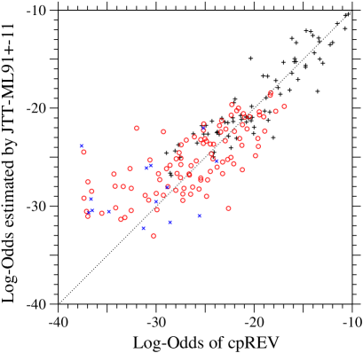
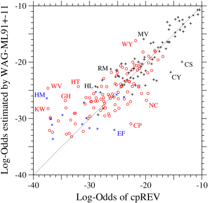
C                                                                                                                                          D

     

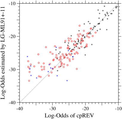
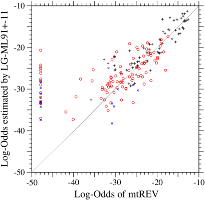
E                                                                                                                                          F

     

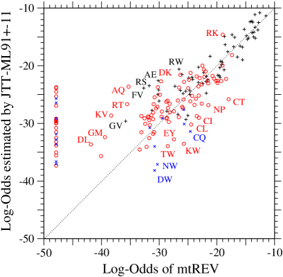
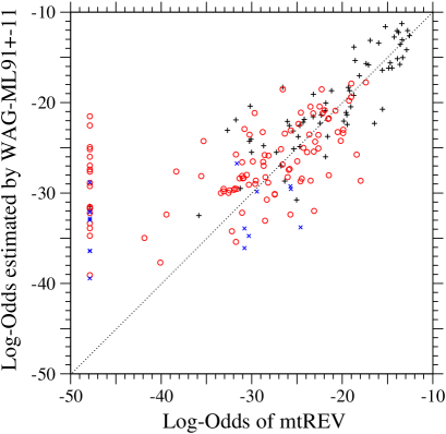
Figure S6: Models fitted to each of cpREV and mtREV. Each element log-$O(\langle S\rangle(\hat{\tau},\hat{\sigma}))_{ab}$ of the log-odds matrix of the model fitted to each empirical substitution matrix is plotted against the log-odds log-$O(S^{{\mbox{\scriptsize obs}}}(\mbox{1 PAM}))_{ab}$ calculated from the corresponding empirical substitution matrix. Plus, circle, and cross marks show the log-odds values for one-, two-, and three-step amino acid pairs, respectively. The dotted line in each figure shows the line of equal values between the ordinate and the abscissa.

A                                                                                                                                                B

     

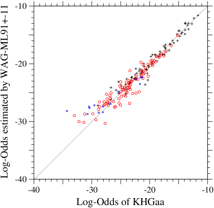
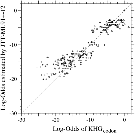
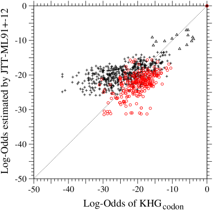
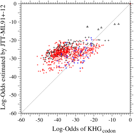
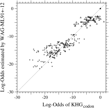
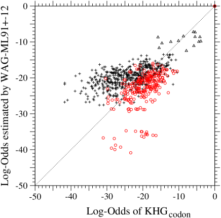
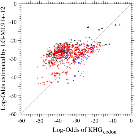
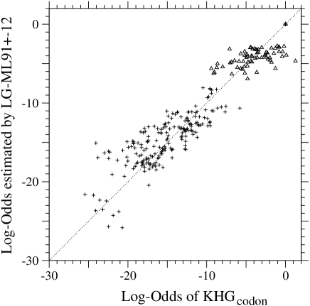
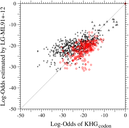
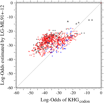
C

Figure S7: Models fitted to the KHG-derived amino acid substitution matrix. Each element log-$O(\langle S\rangle(\hat{\tau},\hat{\sigma}))_{ab}$ of the log-odds matrix of the model fitted to the 1-PAM KHG-derived amino acid substitution matrix (KHGaa) is plotted against the log-odds log-$O(S^{{\mbox{\scriptsize obs}}}(\mbox{1 PAM}))_{ab}$ calculated from KHGaa. Plus, circle, and cross marks show the log-odds values for one-, two-, and three-step amino acid pairs, respectively. The dotted line in each figure shows the line of equal values between the ordinate and the abscissa.

A                                                                                                                                                B

     

C

Figure S8: The JTT-ML91+-12 model fitted to the 1-PAM KHG codon substitution matrix. Each element log-$O(\langle S\rangle(\hat{\tau},\hat{\sigma}))_{\mu\nu}$ of the log-odds matrix corresponding to (A) single, (B) double, and (C) triple nucleotide changes in the JTT-ML91+-12 model fitted to the 1-PAM KHG codon substitution matrix is plotted against the log-odds log-$O(S^{{\mbox{\scriptsize KHG}}}(\mbox{1 PAM}))_{\mu\nu}$ calculated from KHG. Upper triangle, plus, circle, and cross marks show the log-odds values for synonymous pairs and one-, two-, and three-step amino acid pairs, respectively. The dotted line in each figure shows the line of equal values between the ordinate and the abscissa.

A                                                                                                                                                B

     

C

Figure S9: The WAG-ML91+-12 model fitted to the 1-PAM KHG codon substitution matrix. Each element log-$O(\langle S\rangle(\hat{\tau},\hat{\sigma}))_{\mu\nu}$ of the log-odds matrix corresponding to (A) single, (B) double, and (C) triple nucleotide changes in the WAG-ML91+-12 model fitted to the 1-PAM KHG codon substitution matrix is plotted against the log-odds log-$O(S^{{\mbox{\scriptsize KHG}}}(\mbox{1 PAM}))_{\mu\nu}$ calculated from KHG. Upper triangle, plus, circle, and cross marks show the log-odds values for synonymous pairs and one-, two-, and three-step amino acid pairs, respectively. The dotted line in each figure shows the line of equal values between the ordinate and the abscissa.

A                                                                                                                                                B

     

C

Figure S10: The LG-ML91+-12 model fitted to the 1-PAM KHG codon substitution matrix. Each element log-$O(\langle S\rangle(\hat{\tau},\hat{\sigma}))_{\mu\nu}$ of the log-odds matrix corresponding to (A) single, (B) double, and (C) triple nucleotide changes in the LG-ML91+-12 model fitted to the 1-PAM KHG codon substitution matrix is plotted against the log-odds log-$O(S^{{\mbox{\scriptsize KHG}}}(\mbox{1 PAM}))_{\mu\nu}$ calculated from KHG. Upper triangle, plus, circle, and cross marks show the log-odds values for synonymous pairs and one-, two-, and three-step amino acid pairs, respectively. The dotted line in each figure shows the line of equal values between the ordinate and the abscissa.

A

Table S1: ML estimates of the present models without selective constraints on amino acids for the 1-PAM substitution matrices of JTT, WAG, cpREV, and mtREV.

		JTT		WAG		cpREV		mtREV
		No-Constraints- a		No-Constraints- a		No-Constraints- a		No-Constraints- a
id no.	parameter	1	10	1	10	1	10	1	10
0	$-\hat{w}_{0}$	(0.0)	(0.0)	(0.0)	(0.0)	(0.0)	(0.0)	(0.0)	(0.0)
1	$1/\hat{\beta}$	($\infty$)	($\infty$)	($\infty$)	($\infty$)	($\infty$)	($\infty$)	($\infty$)	($\infty$)
2	$\hat{m}_{[tc][ag]}$	($\rightarrow 0$)	$\rightarrow 0$	($\rightarrow 0$)	0.279	($\rightarrow 0$)	0.0455	($\rightarrow 0$)	0.0405
3	$\hat{m}_{tc|ag}/\hat{m}_{[tc][ag]}$	2.16	2.20	1.61	1.54	2.17	2.62	2.32	3.24
4	$\hat{m}_{ag}/\hat{m}_{tc|ag}$	(1.0)	1.28	(1.0)	1.36	(1.0)	1.50	(1.0)	1.47
5	$\hat{m}_{ta}/\hat{m}_{[tc][ag]}$	(1.0)	0.629	(1.0)	0.687	(1.0)	0.480	(1.0)	0.595
6	$\hat{m}_{tg}/\hat{m}_{[tc][ag]}$	(1.0)	0.708	(1.0)	0.622	(1.0)	0.775	(1.0)	0.373
7	$\hat{m}_{ca}/\hat{m}_{[tc][ag]}$	(1.0)	1.28	(1.0)	1.45	(1.0)	1.64	(1.0)	1.96
8	$\hat{f}^{{\mbox{\scriptsize mut}}}_{t+a}$	(0.5)	0.495	(0.5)	0.401	(0.5)	0.279	(0.5)	0.226
9	$\hat{f}^{{\mbox{\scriptsize mut}}}_{t}/\hat{f}^{{\mbox{\scriptsize mut}}}_{t+a}$	(0.5)	0.486	(0.5)	0.503	(0.5)	0.563	(0.5)	0.583
10	$\hat{f}^{{\mbox{\scriptsize mut}}}_{c}/\hat{f}^{{\mbox{\scriptsize mut}}}_{c+g}$	(0.5)	0.335	(0.5)	0.354	(0.5)	0.306	(0.5)	0.223
14	$\hat{\sigma}$	($\rightarrow 0$)	1.76	($\rightarrow 0$)	1.58	($\rightarrow 0$)	2.96	($\rightarrow 0$)	2.46
	$\hat{\tau}\hat{\sigma}$	0.0137	0.0228	0.0136	0.0206	0.0139	0.0296	0.0149	0.0296
	#parameters	21	30	21	30	21	30	21	30
	$\hat{I}_{KL}(\hat{\mbox{\boldmath{$\theta$}}})\times 10^{8}\ {}^{b}$	$729533$	207260	$1156393$	233841	$1014962$	249448	$945289$	305500
	$\Delta\mbox{AIC}\ ^{c}$	86428.1	24595.5	37917.6	7719.1	3478.0	904.5	2644.1	901.0
	Ratio of substitution rates
	per codon
	the total base/codon	1.0	1.30	1.0	1.47	1.0	1.40	1.0	1.35
	transition/transversion	1.13	1.00	0.848	0.752	1.11	1.02	1.24	1.10
	nonsynonymous/synonymousd	2.75	4.15	2.84	5.77	2.60	4.91	2.09	3.30
	Ratio of substitution rates
	per codon for $\sigma\rightarrow 0$
	the total base/codon	1.0	1.0	1.0	1.21	1.0	1.04	1.0	1.02
	transition/transversion	1.13	1.20	0.848	0.853	1.11	1.43	1.24	1.45
	nonsynonymous/synonymousd	2.75	2.83	2.84	4.26	2.60	3.19	2.09	2.08

^a In all models, equal codon usage ($\hat{f}^{{\mbox{\scriptsize usage}}}_{t}=\hat{f}^{{\mbox{\scriptsize usage}}}_{a}=\hat{f}^{{\mbox{\scriptsize usage}}}_{c}=\hat{f}^{{\mbox{\scriptsize usage}}}_{g}=0.25$) is assumed. If the value of a parameter is parenthesized, the parameter is not variable but fixed to the value specified.

^b $\hat{I}_{KL}(\hat{\mbox{\boldmath{$\theta$}}})=-(\ell(\hat{\mbox{\boldmath{$\theta$}}})/N+2.98607330)$ for JTT, $-(\ell(\hat{\mbox{\boldmath{$\theta$}}})/N+2.97444860)$ for WAG, $-(\ell(\hat{\mbox{\boldmath{$\theta$}}})/N+2.95801048)$ for cpREV, and $-(\ell(\hat{\mbox{\boldmath{$\theta$}}})/N+2.85313622)$ for mtREV; see text for details.

^c $\Delta\mbox{AIC}\equiv 2N\hat{I}_{KL}(\hat{\mbox{\boldmath{$\theta$}}})+2\times$ #parameters with $N\simeq 5919000$ for JTT, $N\approx 1637663$ for WAG, $N\approx 169269$ for cpREV and $N\approx 137637$ for mtREV; see text for details.

^d Note that these ratios are not the ratios of the rates per site but per codon; see text for details.

Table S2: ML estimates of the present models with the selective constraints based on mean energy increments due to an amino acid substitution (EI) for the 1-PAM substitution matrices of JTT, WAG, cpREV, and mtREV.

	JTT		WAG		cpREV		mtREV
	EI-10 a	EI-11 a	EI-10 a	EI-11 a	EI-10 a	EI-11 a	EI-10 a	EI-11 a
$-\hat{w}_{0}$	(0.0)	(0.0)	(0.0)	(0.0)	(0.0)	(0.0)	(0.0)	(0.0)
$1/\hat{\beta}$	2.50	2.60	1.78	2.14	2.15	2.26	2.14	2.29
$\hat{m}_{[tc][ag]}$	($\rightarrow 0$)	0.308	($\rightarrow 0$)	0.916	($\rightarrow 0$)	0.684	($\rightarrow 0$)	0.737
$\hat{m}_{tc|ag}/\hat{m}_{[tc][ag]}$	2.51	2.22	1.82	1.58	2.82	2.24	4.21	3.06
$\hat{m}_{ag}/\hat{m}_{tc|ag}$	1.01	1.01	1.13	1.10	1.19	1.14	1.05	1.01
$\hat{m}_{ta}/\hat{m}_{[tc][ag]}$	1.02	1.07	1.26	1.22	0.992	1.14	1.48	1.44
$\hat{m}_{tg}/\hat{m}_{[tc][ag]}$	1.06	1.09	0.985	1.01	1.34	1.23	0.792	0.797
$\hat{m}_{ca}/\hat{m}_{[tc][ag]}$	0.937	0.891	1.04	0.949	0.974	0.925	1.17	1.08
$\hat{f}^{{\mbox{\scriptsize mut}}}_{t+a}$	0.582	0.565	0.516	0.486	0.376	0.405	0.359	0.403
$\hat{f}^{{\mbox{\scriptsize mut}}}_{t}/\hat{f}^{{\mbox{\scriptsize mut}}}_{t+a}$	0.522	0.525	0.603	0.575	0.647	0.642	0.671	0.646
$\hat{f}^{{\mbox{\scriptsize mut}}}_{c}/\hat{f}^{{\mbox{\scriptsize mut}}}_{c+g}$	0.432	0.450	0.495	0.511	0.450	0.462	0.388	0.404
$\hat{\sigma}$	3.20	0.918	11.7	0.998	7.26	0.969	5.25	0.339
$\hat{\tau}\hat{\sigma}$	0.0358	0.0217	0.0709	0.0204	0.0558	0.0211	0.0531	0.0185
#parameters	30	31	30	31	30	31	30	31
$\hat{I}_{KL}(\hat{\mbox{\boldmath{$\theta$}}})\times 10^{8}\ {}^{b}$	$129885$	$126178$	144772	126415	180379	169548	233525	222441
$\Delta\mbox{AIC}\ ^{c}$	15435.7	14999.0	4801.8	4202.5	670.7	636.0	702.8	674.3
Ratio of substitution rates
per codon
the total base/codon	1.36	1.35	1.53	1.54	1.45	1.48	1.38	1.44
transition/transversion	1.09	1.11	0.803	0.834	1.08	1.13	1.34	1.41
nonsynonymous/synonymousd	2.09	2.13	2.48	2.82	2.45	2.65	1.75	1.92
Ratio of substitution rates per codon
for $\sigma\rightarrow 0$
total base/codon	1,0	1.18	1.0	1.38	1.0	1.31	1.0	1.37
transition/transversion	1.49	1.28	1.25	0.944	1.93	1.36	2.35	1.56
nonsynonymous/synonymousd	1.12	1.59	0.945	2.13	1.15	1.99	0.767	1.64
Ratio of substitution rates per codon
for $w_{ab}=0$ and $\sigma\rightarrow 0$
total base/codon	1.0	1.28	1.0	1.59	1.0	1.48	1.0	1.59
transition/transversion	1.31	1.15	0.983	0.830	1.51	1.50	2.15	1.57
nonsynonymous/synonymousd	2.57	3.83	2.82	6.53	2.74	1.16	1.84	4.51

^a In all models, equal codon usage ( $\hat{f}^{{\mbox{\scriptsize usage}}}_{t}=\hat{f}^{{\mbox{\scriptsize usage}}}_{a}=\hat{f}^{{\mbox{\scriptsize usage}}}_{c}=\hat{f}^{{\mbox{\scriptsize usage}}}_{g}=0.25$ ) is assumed. If the value of a parameter is parenthesized, the parameter is not variable but fixed to the value specified.

^b $\hat{I}_{KL}(\hat{\mbox{\boldmath{$\theta$}}})=$ $-(\ell(\hat{\mbox{\boldmath{$\theta$}}})/N+2.98607330)$ for JTT, $-(\ell(\hat{\mbox{\boldmath{$\theta$}}})/N+2.97444860)$ for WAG, $-(\ell(\hat{\mbox{\boldmath{$\theta$}}})/N+2.95801048)$ for cpREV, and $-(\ell(\hat{\mbox{\boldmath{$\theta$}}})/N+2.85313622)$ for mtREV; see text for details.

^c $\Delta\mbox{AIC}\equiv 2N\hat{I}_{KL}(\hat{\mbox{\boldmath{$\theta$}}})+2\times$ #parameters with $N\simeq 5919000$ for JTT, $N\approx 1637663$ for WAG, $N\approx 169269$ for cpREV, and $N\approx 137637$ for mtREV; see text for details.

^d Note that these ratios are not the ratios of the rates per site but per codon; see text for details.

Table S3: ML estimates of the present models with the selective constraints based on the Grantham’s and the Miyata’s amino acid distances for the 1-PAM substitution matrices of JTT and WAG.

	JTT				WAG
	Grantham- a		Miyata- a		Grantham- a		Miyata- a
	10	11	10	11	10	11	10	11
$-\hat{w}_{0}$	(0.0)	(0.0)	(0.0)	(0.0)	(0.0)	(0.0)	(0.0)	(0.0)
$1/\hat{\beta}$	82.0	81.9	1.71	1.82	58.9	65.1	1.28	1.59
$\hat{m}_{[tc][ag]}$	($\rightarrow 0$)	0.0392	($\rightarrow 0$)	0.617	($\rightarrow 0$)	0.353	($\rightarrow 0$)	1.33
$\hat{m}_{tc|ag}/\hat{m}_{[tc][ag]}$	2.12	2.09	2.32	1.92	1.49	1.44	1.64	1.40
$\hat{m}_{ag}/\hat{m}_{tc|ag}$	1.08	1.08	1.05	1.05	1.18	1.17	1.15	1.11
$\hat{m}_{ta}/\hat{m}_{[tc][ag]}$	0.864	0.863	0.925	0.983	0.987	0.938	1.02	1.02
$\hat{m}_{tg}/\hat{m}_{[tc][ag]}$	0.961	0.983	0.922	0.985	0.816	0.907	0.813	0.912
$\hat{m}_{ca}/\hat{m}_{[tc][ag]}$	1.16	1.16	1.26	1.12	1.39	1.32	1.55	1.23
$\hat{f}^{{\mbox{\scriptsize mut}}}_{t+a}$	0.582	0.581	0.574	0.543	0.528	0.517	0.499	0.466
$\hat{f}^{{\mbox{\scriptsize mut}}}_{t}/\hat{f}^{{\mbox{\scriptsize mut}}}_{t+a}$	0.512	0.513	0.513	0.505	0.573	0.562	0.575	0.531
$\hat{f}^{{\mbox{\scriptsize mut}}}_{c}/\hat{f}^{{\mbox{\scriptsize mut}}}_{c+g}$	0.384	0.385	0.448	0.479	0.412	0.420	0.513	0.541
$\hat{\sigma}$	2.80	2.37	2.98	$0.00938$	9.00	2.97	9.87	$0.00118$
$\hat{\tau}\hat{\sigma}$	0.0330	0.0306	0.0342	0.0147	0.0596	0.0317	0.0632	0.0135
#parameters	30	31	30	31	30	31	30	31
$\hat{I}_{KL}(\hat{\mbox{\boldmath{$\theta$}}})\times 10^{8}\ {}^{b}$	$157835$	157281	$138419$	$130721$	173694	168463	154639	133347
$\Delta\mbox{AIC}\ ^{c}$	18744.5	18680.9	16446.1	15536.8	5749.0	5579.7	5124.9	4429.5
Ratio of substitution rates per codon
the total base/the total codon	1.35	1.35	1.35	1.34	1.51	1.50	1.51	1.53
transition/transversion	1.04	1.04	1.07	1.10	0.768	0.779	0.791	0.812
nonsynonymous/synonymousd	2.21	2.20	2.14	2.18	2.54	2.65	2.53	2.93
Ratio of substitution rates per codon
for $\sigma\rightarrow 0$
the total base/the total codon	1.0	1.02	1.0	1.33	1.0	1.16	1.0	1.53
transition/transversion	1.33	1.31	1.42	1.10	1.06	0.951	1.17	0.813
nonsynonymous/synonymousd	1.22	1.28	1.17	2.17	1.04	1.52	1.02	2.93
Ratio of substitution rates per codon
for $w_{ab}=0$ and $\sigma\rightarrow 0$
the total base/the total codon	1.0	1.04	1.0	1.48	1.0	1.26	1.0	1.74
transition/transversion	1.12	1.10	1.21	0.990	0.803	0.771	0.881	0.736
nonsynonymous/synonymousd	2.67	2.81	2.63	5.24	2.97	4.20	2.92	8.49

^a In all models, equal codon usage ($\hat{f}^{{\mbox{\scriptsize usage}}}_{t}=\hat{f}^{{\mbox{\scriptsize usage}}}_{a}=\hat{f}^{{\mbox{\scriptsize usage}}}_{c}=\hat{f}^{{\mbox{\scriptsize usage}}}_{g}=0.25$) is assumed. If the value of a parameter is parenthesized, the parameter is not variable but fixed to the value specified.

^b $\hat{I}_{KL}(\hat{\mbox{\boldmath{$\theta$}}})=-(\ell(\hat{\mbox{\boldmath{$\theta$}}})/N+2.98607330)$ for JTT, and $-(\ell(\hat{\mbox{\boldmath{$\theta$}}})/N+2.97444860)$ for WAG; see text for details.

^c $\Delta\mbox{AIC}\equiv 2N\hat{I}_{KL}(\hat{\mbox{\boldmath{$\theta$}}})+2\times$ #parameters with $N=5919000$ for JTT, and $N\approx 1637663$ for WAG; see text for details.

^d Note that these ratios are not the ratios of the rates per site but per codon; see text for details.

References

- 1. Kimura M (1980) A simple model for estimating evolutionary rates of base substitutions through comparative studies of nucleotide sequences. J Mol Evol 16: 111-120.
- 2. Hasegawa M, Kishino H, Yano T (1985) Dating of the human-ape splitting by a molecular clock of mitochondrial dna. J Mol Evol 22: 160-174.
- 3. Tamura K, Nei M (1993) Estimation of the number of nucleotide substitutions in the control region of mitochondrial dna in humans and chimpanzees. Mol Biol Evol 10: 512-526.
- 4. Dayhoff MO, Schwartz RM, Orcutt BC (1978) A model of evolutionary change in proteins. In: Dayhoff MO, editor, Atlas of protein sequence and structure, Washington D.C.: National Biomedical Research Foundation, volume 5. Suppl. 3 edition, pp. 345-352.
- 5. Jones DT, Taylor WR, Thornton JM (1992) The rapid generation of mutation data matrices from protein sequences. CABIOS 8: 275-282.
- 6. Adachi J, Hasegawa M (1996) Model of amino acid substitution in proteins encoded by mitochondrial dna. J Mol Evol 42: 459-468.
- 7. Yang Z, Nielsen R, Hasegawa M (1998) Models of amino acid substitution and application to mitochondrial protein evolution. Mol Biol Evol 15: 1600-1611.
- 8. Adachi J, Waddell PJ, Martin W, Hasegawa M (2000) Plastid genome phylogeny and a model of amino acid substitution for proteins encoded by chloroplast dna. J Mol Evol 50: 348-358.
- 9. Dimmic MW, Mindell DP, Goldstein RA (2000) Modelling evolution at the protein level using an adjustable amino acid fitness model. Pacific Symposium on Biocomputing 5: 18-29.
- 10. Whelan S, Goldman N (2001) A general empirical model of protein evolution derived from multiple protein families using a maximum-likelihood approach. Mol Biol Evol 18: 691-699.
- 11. Le SQ, Gascuel O (2008) An improved general amino acid replacement matrix. Mol Biol Evol 25: 1307-1320.
- 12. Huelsenbeck JP, Joyce P, Lakner C, Ronquist F (2008) Bayesian analysis of amino acid substitution models. Phil Trans R Soc B 363: 3941-3953.
- 13. Schneider A, Cannarozzi GM, Gonnet GH (2005) Empirical codon substitution matrix. BMC Bioinformatics 6: 134.
- 14. Kosiol C, Holmes I, Goldman N (2007) An empirical codon model for protein sequence evolution. Mol Biol Evol 24: 1464-1479.
- 15. Delport W, Scheffler K, Gravenor MB, Muse SV, Kosakovsky Pond S (2010) Benchmarking multi-rate codon models. PLos One 5: e11587.
- 16. Delport W, Scheffler K, Botha G, Gravenor MB, Muse SV, et al. (2010) Codontest: Modeling amino acid substitution preferences in coding sequences. PLos Comp Biol 6: e1000885.
- 17. Miyazawa S, Jernigan RL (1993) A new substitution matrix for protein sequence searches based on contact frequencies in protein structures. Protein Eng 6: 267-278.
- 18. Goldman N, Yang Z (1994) A codon-based model of nucleotide substitution for protein-coding dna. Mol Biol Evol 11: 725-736.
- 19. Muse SV, Gaut BS (1994) A likelihood approach for comparing synonymous and nonsynonymous nucleotide substitution rates, with application to the chloroplast genome. Mol Biol Evol 11: 715-724.
- 20. Whelan S, Goldman N (2004) Estimating the frequency of events that cause multiple-nucleotide changes. Genetics 167: 2027-2043.
- 21. Doron-Faigenboim A, Pupko T (2007) A combined empirical and mechanistic codon model. Mol Biol Evol 24: 388-397.
- 22. Yang Z, Nielsen R (2008) Mutation-selection models of codon substitution and their use to estimate selective strengths on codon usage. Mol Biol Evol 25: 568-579.
- 23. Seo TK, Kishino H (2008) Synonymous substitutions substantially improve evolutionary inference from highly diverged proteins. Syst Biol 57: 367-377.
- 24. Seo TK, Kishino H (2009) Statistical comparison of nucleotide, amino acid, and codon substitution models for evolutionary analysis of protein-coding sequences. Syst Biol 58: 199-210.
- 25. Jin L, Nei M (1990) Limitations of the evolutionary parsimony method of phylogeny analysis. Mol Biol Evol 7: 82-102.
- 26. Yang Z (1993) Maximum-likelihood estimation of phylogeny from dna sequences when substitution rates differ over time. Mol Biol Evol 10: 1396-1401.
- 27. Averof M, Rokas A, Wolfe KH, Sharp PM (2000) Evidence for a high frequency of simultaneous double-nucleotide substitutions. Science 287: 1283-1286.
- 28. Smith NGC, Webster MT, Ellegren H (2003) A low rate of simultaneous double-nucleotide mutations in primates. Mol Biol Evol 20: 47-53.
- 29. Bazykin G, Kondrashov F, Ogurtsov A, Sunyaev S, Kondrashov A (2004) Positive selection at sites of multiple amino acid replacements since rat-mouse divergence. Nature 429: 558-562.
- 30. Anisimova M, Kosiol C (2009) Investigating protein-coding sequence evolution with probabilistic codon substitution models. Mol Biol Evol 26: 255-271.
- 31. Grantham R (1974) Amino acid difference formula to help explain protein evolution. Science 185: 862-864.
- 32. Miyata T, Miyazawa S, Yasunaga T (1979) Two type of amino acid substitutions in protein evolution. J Mol Evol 12: 219-236.
- 33. Choi SC, Hobolth A, Robinson DM, Kishino H, Thorne JL (2007) Quantifying the impact of protein tertiary structure on molecular evolution. Mol Biol Evol 24: 1769-1782.
- 34. Conant GC, Wagner GP, Stadler PF (2007) Modeling amino acid substitution patterns in orthologous and paralogous genes. Mol Phylogenet Evol 42: 298-307.
- 35. Takahata N (1987) On the overdispersed molecular clock. Genetics 116: 169-179.
- 36. Rodrigue N, Lartillot N, Philippe H (2008) Bayesian comparisons of codon substitution models. Genetics 180: 1579-1591.
- 37. Akaike H (1974) A new look at the statistical model identification. IEEE Trans Autom Contr AC-19: 716-723.
- 38. Whelan S, de Bakker P, Quevillon E, Rodriguez N, Goldman N (2006) Pandit: an evolution-centric database of protein and associated nucleotide domains with inferred trees. Nucl Acid Res 34: D327-D331.
- 39. Miyata T, Yasunaga T (1980) Molecular evolution of mrna: a method for estimating evolutionary rates of synonymous and amino acid substitutions from homologous nucleotide sequences and its applications. J Mol Evol 16: 23-36.
- 40. Halpern AL, Bruno WJ (1998) Evolutionary distances for protein-coding sequences: modeling site-specific residue frequencies. Mol Biol Evol 15: 910-917.
- 41. Keller I, Bensasson D, Nichols RA (2007) Transition-transversion bias is not universal: A counter example from grasshopper pseudogenes. PLoS Genet 3: 0185-0191.
- 42. Larkin MA, Blackshields G, Brown NP, Chenna R, McGettigan PA, et al. (2007) Clustalw and clustalx version 2.0. Bioinformatics 23: 2947-2948.
- 43. Guindon S, Gascuel O (2003) Simple, fast, and accurate algorithm to estimate large phylogenies by maximum likelihood. Systematic Biol 52: 696-704.
- 44. Yang Z (1994) Maximum likelihood phylogenetic estimation from dna sequences with variable rates over sites: approximate methods. J Mol Evol 39: 306-314.
- 45. Kinjo AR, Nishikawa K (2004) Eigenvalue analysis of amino acid substitution matrices reveals a sharp transition of the mode of sequence conservation in proteins. Bioinformatics 20: 2504-2508.
- 46. Miyazawa S, Jernigan RL (2003) Long- and short-range interactions in native protein structures are consistent/minimally frustrated in sequence space. Proteins 50: 35-43.
- 47. Kimura M, Ohta T (1974) On some principles governing molecular evolution. Proc Natl Acad Sci USA 71: 2848-2852.
- 48. Miyazawa S, Jernigan RL (1999) Self-consistent estimation of inter-residue protein contact energies based on an equilibrium mixture approximation of residues. Proteins 34: 49-68.
- 49. Miyazawa S, Jernigan RL (1996) Residue-residue potentials with a favorable contact pair term and an unfavorable high packing density term for simulation and threading. J Mol Biol 256: 623-644.
- 50. Miyazawa S, Jernigan RL (1985) Estimation of effective interresidue contact energies from protein crystal structures: Quasi-chemical approximation. Macromolecules 18: 534-552.
- 51. Tsai J, Taylor R, Chothia C, Gerstein M (1999) The packing density in proteins: standard radii and volumes. J Mol Biol 290: 253-266.
- 52. Lanave C, Preparata G, Saccone C, Serio G (1984) A new method for calculating evolutionary substitution rates. J Mol Evol 20: 86-93.
- 53. Felsenstein J (2004) Inferring Phylogenies. Massachusetts: Sinauer Associates, Inc.
- 54. Mizuguchi K, Deane CM, Blundell TL, Overington JP (1998) Homstrad: a database of protein structure alignments for homologous families. Protein Sci 7: 2469-2471.
- 55. Henikoff S, Henikoff JG (1992) Amino acid substitution matrices from protein blocks. Proc Natl Acad Sci USA 89: 10915-10919.
A B
A B
C D
A B
A B
C D