Exciton condensation and fractional charge in a bilayer two-dimension electron gas adjacent to a superconductor film

Abstract

We study the exciton condensate (EC) in a bilayer two-dimension-electron-gas (2DEG) adjacent to a type-II superconductor thin film with an array of pinned vortex lattices. By applying continuum low energy theory and carrying numerical simulations of lattice model within mean-field approximation, we find that if the order parameter of EC has a vortex profile, there are exact zero modes and associated rational fractional charge for zero pseudospin potential ($\mu$) and average chemical potential ($h$): $\mu$=$0$ and $h$=$0$; while for $\mu\mathtt{\neq}0$ and $h$=$0$, intervalley mixing splits the zero energy levels, and the system exhibits irrational fractional axial charge.

Introduction Charge fractionalization and fractional statistics wilczek in two-dimensional systems have attracted much attention due to their potential applications in topological quantum computation fw1 ; fw2 ; fw3 . One representative example is the well known $\nu$=$\frac{5}{2}$ fractional quantum Hall $($FQH$)$ system Read . The excitations of the $\nu$=$\frac{5}{2}$ FQH system carry fractional charge and exhibit non-Abelian fractional statistics. The pivotal features of FQH system are strong correlations and broken time-reversal symmetry $($TRS$)$ as a result of the electrons’ strong coulomb interaction and strong external magnetic field. However, some recently proposed models Hou ; Franz have revealed that the strong correlations and broken TRS are not necessary for fractionalization. Moreover, these models indicate that the nontrivial topological configurations play a key role in the fractionalization. The common features of these models are that the TRS is not broken, and the low energy excitations can be described by the Dirac field coupling with a topologically nontrivial scalar field (vortex profiles, for instance) Jackiw . Therefore, the energy spectrum’s symmetry and index theorem of the Dirac operator protect the zero modes and the associated fractionalization Chamon . In another interesting model Weeks different from aforementioned ones, the fractionalization of the excitations is due to the response to the half-magnetic-flux-quanta defect of the system in the integer quantum hall (IQH) regime. This model is more likely to be fabricated compared to aforementioned systems.

We start with a bilayer two-dimension-electron-gas (2DEG), as illustrated schematically in Fig. 1(a). Each layer is adjacent to a film of type-$\Pi$ superconductor supplying the quantization of flux in unit of $\frac{1}{2}\Phi_{0}$ ($\Phi_{0}$=$h/e$) by the Abrikosov vortex square lattices. The spin-polarized electrons in the bilayer are almost localized near the Abrikosov vortex cores. At half filling (namely, the number of electrons is one half of the total lattice sites), the bilayer system has a magnetic filling factor of two, and the magnetic flux through one square lattice cell is $\pi$. In addition, the two layers are separated by a spacer which is usually a dielectric barrier (e.g., SiO₂). The chemical potential in each layer can be adjusted independently by the respective gate voltage. The carrier in each layer has electron or hole nature determined by the respective band structure. In particular, the inverse external gate voltages in two layers bias the charge balance of two layers and result in the perfect particle-hole symmetry. So the electrons in one layer and holes in another layer bound together and form exciton condensate $($EC$)$ due to the interlayer coulomb interaction. Our system is favorable for EC because of the strong magnetic field and low electron density as suggested by experiments of the coupled quantum wells Fuku Eisen .

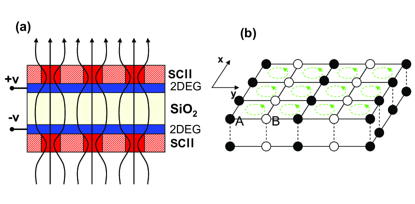
Figure 1: (Color online) (a) Schematic structure of exciton condensate system. The external gates induce the symmetric electron and hole carriers. (b) Our bilayer square lattice model.

In this paper, we construct a tight-binding model analogous to bilayer graphene Franz1 and solve the Bogoliubov-de Gennes (BdG) equation self-consistently in real space to determine the amplitude of EC order parameter (OP) and study the system’s topological properties originating from OP with vortex configuration. The low energy excitations of the system present novel features due to the vortex configuration in OP. We show that when the biased voltage is zero, two degenerate fermion zero modes (each one for one valley) emerge. Furthermore, for the vortex with vorticity ($n$=1) at half filling, each layer has fractional charge $\frac{1}{2}e$ or $-\frac{1}{2}e$ (depending on whether the two zero modes are occupied or not), though the total and difference charge of bilayer are the integer numbers. When the biased voltage is not zero, the two fermion zero modes slightly and symmetrically split around zero energy due to the intervalley mixing. At half filling, the axial charge of the whole system is fractional just as what happens in bilayer graphene studied in Ref. (13).

Lattice model and exciton condensation In the following, we present a model to describe the EC in our system at near zero temperature. The essential terms include intralayer hopping between the nearest neighbor sites. We ignore the intralayer carriers’ Coulomb interactions because their effects only renormalize the energy bands. We consider interlayer Coulomb repulsion as an effective short-range repulsion only between interlayer electrons at the same planar sites. Furthermore, the external biased voltage is included. Since the electron spin is polarized along the direction of the magnetic field, we omit spin index. There is no direct hopping between the two layers.

The Hamiltonian of our system can be expressed as follows

$$H=\underset{i\alpha}{-\sum}\mu_{\alpha}n_{i\alpha}-\underset{<i,j>\alpha}{\sum}t_{ij\alpha}e^{i\theta_{ij\alpha}}c_{j\alpha}^{+}c_{i\alpha}$$

$$+U\underset{i}{\sum}n_{i1}n_{i2}.$$ (1)

Here $c_{i\alpha}$ annihilates an electron at site $i$ of layer-$\alpha$ ($\alpha$=$1,2$), $n_{i\alpha}$=$c_{i\alpha}^{+}c_{i\alpha}$, and $t_{ij\alpha}$ is intralayer nearest-neighbor hopping with $t_{ij1}$=$t_{ij2}$ for the electron-electron bilayer and $t_{ij1}$=$-t_{ij2}$ for electron-hole bilayer. We consider the electron-hole bilayer and set $t_{ij1}$=$-t_{ij2}\mathtt{\equiv}t$=$1$. $\mu_{\alpha}$ is the chemical potential of layer-$\alpha$. The magnetic field is included through the Peierls phase factors, $\theta_{ij\alpha}$=$\frac{2\pi}{\Phi_{0}}\int_{\mathbf{r}_{i\alpha}}^{\mathbf{r}_{j\alpha}}\mathbf{A}_{\alpha}\mathtt{\cdot}d\mathbf{l}$. We choose to work in Landau gauge $\mathbf{A}_{\alpha}$=$\frac{1}{2}\Phi_{0}(-y,0),$ where we have set the lattice space unity. The mean-field order parameter of the EC is $\Delta_{i}$=$U\left\langle c_{i2}^{+}c_{i1}\right\rangle$ , and the mean-field Hamiltonian is

$$H_{MF} =-\underset{i\alpha}{\sum}\mu_{\alpha}n_{i\alpha}+\underset{<i,j>\alpha}{\sum}(-)^{\alpha}te^{i\theta_{ij\alpha\beta}}c_{j\alpha}^{+}c_{i\alpha}$$

$$-\underset{i}{\sum}(\Delta_{i}c_{i1}^{+}c_{i2}+h.c.)+\frac{1}{U}\underset{i}{\sum}\left|\Delta_{i}\right|^{2}.$$ (2)

With the help of the following Bogoliubov transformation

$$\left[\begin{array}[c]{c}c_{i1}\\ c_{i2}\end{array}\right]=\underset{n}{\sum}\left[\begin{array}[c]{cc}u_{i}^{n}&-\upsilon_{i}^{n\ast}\\ \upsilon_{i}^{n}&u_{i}^{n\ast}\end{array}\right]\left[\begin{array}[c]{c}\alpha_{n}\\ \beta_{n}^{+}\end{array}\right],$$ (3)

the above Hamiltonian(2) can be diagonalized by solving the following BdG equation

$$\underset{j}{\sum}\left[\begin{array}[c]{cc}h_{ij,1}&-\Delta_{i}\delta_{ij}\\ -\Delta_{i}^{\ast}\delta_{ij}&h_{ij,2}\end{array}\right]=E_{n}\left[\begin{array}[c]{c}u_{j}^{n}\\ \upsilon_{j}^{n}\end{array}\right],$$ (4)

where $h_{ij,1(2)}=\mp t-\mu_{1(2)}\delta_{ij}$. The self-consistent equation of the OP is

$$\Delta_{i}=-\underset{n}{\sum}u_{i}^{n}\upsilon_{i}^{n\ast}\tanh(\frac{E_{n}}{2k_{B}T}).$$ (5)

We solve the set of BdG equations self-consistently via exact diagonalization in real space. The system size of $24\mathtt{\times}24$ is used in the calculation and the convergence criterion of $\Delta_{i}$ is set to 10^-4 in unit of the intralayer nearest-neighbor hopping. We consider the near-zero temperature and set $k_{B}T$ to be 10^-3. For convenience of discussion, we define the average chemical potential and pseudospin polarization potential as $h$=$(\mu_{1}\mathtt{+}\mu_{2})/2$ and $\mu$=$(\mu_{1}\mathtt{-}\mu_{2})/2$. We find that if $h$=$0$ (we set $\mu_{2}$=$-\mu_{1}$=$-\mu$), the exciton order parameter is uniform: $\Delta_{i}$=$\Delta$=$m$, where $m$ is real. Our calculations show that as $h$ decreases from zero, the phases of system undergo BCS-like phase, 1D modulated Larkin-Ovchinnikov-like (LO) phase LO , 2D modulated LO-like phase and finally OP zero.

In the following, we restrict ourselves to the case of $\mu_{2}$=$-\mu_{1}$=$-\mu$. In the Landau gauge that we choose, the system can be viewed as simplified lattices as depicted in Fig. 1(b). The magnetic unit cell in layer $\alpha$ includes two sites $(l,n)\alpha$ and $(l,n$+$1)\alpha$ denoted by $A\alpha$ and $B\alpha$. The wave functions are of the form of spinor field $\psi(\mathbf{r})$=$[c_{B1}(\mathbf{r}_{l,n+1}),c_{A1}(\mathbf{r}_{l,n}),c_{B2}(\mathbf{r}_{l,n+1}),c_{A2}(\mathbf{r}_{l,n})]^{T}$. In the momentum space with the reduced Brillouin zone $BZ$=$\{k_{y}\mathtt{-}\pi/2\mathtt{\leq}k_{x}\mathtt{\leq}k_{y}$+$\pi/2,\left|k_{y}\right|\mathtt{\leq}\pi\}$, the Hamiltonian can be written as $H_{MF}$=$\sum_{\mathbf{k}}\psi^{+}(\mathbf{k})\mathcal{H}_{MF}(\mathbf{k})\psi(\mathbf{k})$+$E_{0}$ with $E_{0}$= $N_{0}m^{2}/U$ and

$$\mathcal{H}_{MF}(\mathbf{k}) =-\mu\sigma_{3}\otimes I\mathbb{+}2\cos(k_{x})\sigma_{3}\otimes s_{3}-2\cos(k_{y})\sigma_{3}\otimes s_{1}$$

$$-me^{-i\chi\sigma_{3}\otimes I}\sigma_{1}\otimes I,$$ (6)

where $\sigma_{i}$ $(s_{i})$ $(i$=$1,2,3)$ is Pauli matrix acting in sublattice (pseudospin) space and $I$ is unitary matrix. Without loss of generality, we preserve the constant phase $\chi$ of OP. This Hamiltonian possesses the particle-hole symmetry

$$\Omega\mathcal{H}_{MF}(\mathbf{k})\Omega=-\mathcal{H}_{MF}^{\ast}(-\mathbf{k})$$ (7)

with $\Omega$=$-\sigma_{2}\mathtt{\otimes}I$ and $\Omega^{2}$=$1$. As a result of this symmetry, it is easy to find

$$\mathcal{H}_{MF}\Omega\psi^{\ast}=-\Omega\mathcal{H}_{MF}^{\ast}\psi^{\ast}=-E\Omega\psi^{\ast}.$$ (8)

It means that if $\psi$ is an eigenvector of $\mathcal{H}_{MF}$ with eigenvalue $E,$ then $\Omega\psi^{\ast}$ is guaranteed to be an eigenvector of $\mathcal{H}_{MF}$ with eigenvalue $-E$. So, all nonzero eigenvalues of $\mathcal{H}_{MF}$ come in $\pm E$ pairs and the energy spectrum is symmetric about zero energy. For uniform order parameter $m$, the energy spectrum is of the form

$$E(\mathbf{k})=\pm 2\sqrt{(\sqrt{\cos^{2}k_{x}+\cos^{2}k_{y}}\pm\mu)^{2}+m^{2}}.$$ (9)

The energy spectrum symmetry is clear in this case. Note that no in-gap eigenvalues exist as $m\mathtt{\neq}0$ in uniform case.

Zero modes and charge fractionalization We now investigate the low-energy behaviors of our system. In the low energy limit, the properties of the system are dominated by the excitations around the two inequivalent valleys $\mathbf{K}_{\pm}$=$(\mp\frac{\pi}{2},\mp\frac{\pi}{2})$ where $\cos\left.k_{x}\right|_{\mathbf{K}_{\pm}+\mathbf{p}}$=$\pm p_{x}$ and $\cos\left.k_{y}\right|_{\mathbf{K}_{\pm}+\mathbf{p}}$=$\pm p_{y}$. Then, the linearized mean-field Hamiltonian for these excitations are $\mathcal{H}_{MF+}$+$\mathcal{H}_{MF-}$ with $\mathcal{H}_{MF+}$=$-iI\mathtt{\otimes}\sigma_{2}\mathcal{H}_{MF-}iI\mathtt{\otimes}\sigma_{2}\mathtt{\equiv}\mathcal{H}$,

$$\mathcal{H}=-\mu\sigma_{3}\otimes I\mathbb{+}2p_{x}\sigma_{3}\otimes s_{3}-2p_{y}\sigma_{3}\otimes s_{1}-me^{-i\chi\sigma_{3}\otimes I}\sigma_{1}\otimes I.$$ (10)

Here, $\mathbf{p}$=$-i\nabla$ is the momentum operator. Since the valleys are decoupled in the low-energy theory, we first study a single valley.

Around the valleys, the Hamiltonian $\mathcal{H}$ possesses a symmetric property

$$\Xi\mathcal{H}(\mathbf{K}_{\pm}+\mathbf{p})\Xi=\mathcal{H}^{\ast}(\mathbf{K}_{\pm}+\mathbf{p}),$$ (11)

where $\Xi$=$i\sigma_{2}\mathtt{\otimes}s_{2}.$ This symmetry is unbroken only around each valley. The low-energy excitations obey this symmetry around each valley. The case of $\mu$=$0$ is of particular interest. In this situation, the symmetry of our system gets enhanced. It is easy to check that $\Theta\mathcal{H}\Theta$=$-\mathcal{H}$, $\Theta^{2}$=$1$, with $\Theta\mathtt{\equiv}\sigma_{3}\mathtt{\otimes}s_{2}$. This symmetry has important consequences on the number of zero modes.

Now suppose $\Delta$ is also taken to vary with position and consider OP with a symmetric vortex of vorticity $n$, which means $\Delta(r,\theta)$=$m(r)e^{in\theta}$ with $m(r)$ a real function of $r$ and the constant phase $\chi$ omitted by the special gauge choice. In order to get explicitly analytic solutions, we use the well defined vortex profile

$$\Delta(r,\theta)=\left\{\begin{array}[c]{c}m(r)e^{in\theta},r>0\\ 0,r=0\end{array}\right.,$$ (12)

In quantum limit, $m(r)$=$m_{0}$, where $m_{0}$ is a positive real constant. The zero-mode solutions satisfy $\mathcal{H}\psi_{0}$=$0$. Eq. (11) means $\mathcal{H}\Xi\psi^{\ast}$=$-\Xi\mathcal{H}^{\ast}\psi^{\ast}$=$-E\Xi\psi^{\ast}$. For zero modes, we impose $\Xi\psi_{0}^{\ast}$=$\psi_{0}.$ If $\Xi\psi_{0}^{\ast}$=$-\psi_{0}$, then the transformation $\psi_{0}\mathtt{\rightarrow}i\psi_{0}$ brings it back to $\Xi\psi_{0}^{\ast}$=$\psi_{0}$. So, in the zero-energy subspace, we can suppose $\psi_{0}$=$[f,g,ig^{\ast},-if^{\ast}]^{T}$. Hence, we can get two independent equations for zero-mode solutions in quantum limit

$$(-\mu-2i\partial_{x})f+2i\partial_{y}g-im_{0}e^{in\theta}g^{\ast} =0$$

$$(-\mu+2i\partial_{x})g+2i\partial_{y}f+im_{0}e^{in\theta}f^{\ast} =0.$$ (13)

In order to get the symmetric solutions in the presence of the symmetric vortex profile, we introduce new wave functions $\zeta$ and $\xi$ defined by the following equations,

$$\left[\begin{array}[c]{c}f\\ g\\ ig^{\ast}\\ -if^{\ast}\end{array}\right]=\frac{\sqrt{2}}{2}\left[\begin{array}[c]{c}-e^{-i\pi/4}(\zeta+\xi)\\ e^{i\pi/4}(\zeta-\xi)\\ e^{i\pi/4}(\zeta^{\ast}-\xi^{\ast})\\ -e^{-i\pi/4}(\zeta^{\ast}+\xi^{\ast})\end{array}\right].$$ (14)

Then, $\zeta,\xi$ satisfy the following equations in polar coordinate,

$$e^{i\theta}(\partial_{r}+ir^{-1}\partial_{\theta})\zeta-m_{0}/2e^{in\theta}\zeta^{\ast}-i\mu/2\xi =0$$

$$e^{-i\theta}(\partial_{r}-ir^{-1}\partial_{\theta})\xi+m_{0}/2e^{in\theta}\xi^{\ast}-i\mu/2\zeta =0,$$ (15)

which are almost the same as that in Ref. (13). The analogous solutions can be gotten as

$$\zeta=e^{-m_{0}r/2}J_{p}(\mu r/2)e^{ip\theta}\text{ and }\xi=-ie^{-m_{0}r/2}J_{q}(\mu r/2)e^{iq\theta},$$ (16)

which are exponentially decayed Bessal functions and $p$=$q\mathtt{-}1$=$\frac{n-1}{2}$. So, the single valued solutions survive only when $n$ is odd. Hence, one zero-mode solution $\psi_{0}^{(1)}(r)$ can be obtained as $\psi_{0}^{(1)}(r)$=$[\psi_{0B1}^{(1)}(r),\psi_{0A1}^{(1)}(r),\psi_{0B2}^{(1)}(r),\psi_{0A2}^{(1)}(r)]^{T}$=$[f,g,ig^{\ast},-if^{\ast}]^{T}$ together with Eqs. (14) and (16). From the relation $\mathcal{H}_{MF+}$=$-iI\mathtt{\otimes}\sigma_{2}\mathcal{H}_{MF-}iI\mathtt{\otimes}\sigma_{2}$, another zero-mode solution is $\psi_{0}^{(2)}(r)$=$[ig,-if,f^{\ast},g^{\ast}]^{T}$. Note that the particular symmetry (defined by the transformation $\Theta$) for $\mu$=$0$ ensures the $|n|$ zero modes, unlike the single zero mode for odd vortex configuration for $\mu\neq$$0$ Gurarie .

With the help of Eqs. (13), (15) and (16), it is interesting to see that the low energy behavior of our model is similar to that of bilayer graphene. The analogy is not surprising, because after the transformation $h_{MF}(\mathbf{k})$=$S^{+}\mathcal{H}_{MF}(\mathbf{k})S$ with $S$=$\exp(i\pi I\mathtt{\otimes}s_{1}/4)\exp(i\pi I\mathtt{\otimes}s_{3}/4)\exp(i\pi I\mathtt{\otimes}s_{1}/2)$, our mean-field Hamiltonian has the form

$$h_{MF}(\mathbf{k})=-\gamma_{0}(\gamma_{1}2\cos k_{x}+\gamma_{2}2\cos k_{y}+me^{-i\chi\gamma_{5}}+\gamma_{0}\gamma_{5}\mu).$$ (17)

Here in the Weyl representation, the Dirac matrices have the forms: $\gamma_{\mu}$=$i\sigma_{2}\mathtt{\otimes}s_{\mu}$, $\gamma_{0}$=$\sigma_{1}\mathtt{\otimes}I$, $\gamma_{\mu}$=$-i\gamma_{0}\gamma_{1}\gamma_{2}\gamma_{3}$=$\sigma_{3}\mathtt{\otimes}I$. The low-energy form of this Hamiltonian at the two independent valleys is nearly identical to that for bilayer graphene.

A localized zero mode in a gapped system with particle-hole symmetry usually bounds a fractional charge $\pm e/2$ Hou ; Franz ; Jackiw ; Chamon wpsu ; Goldstone . Note that the Hamiltonian of our model in low-energy limit is of the Dirac type with first-order differential operators. Therefore, when $\mu$=$0$, and the OP has the form of a symmetric vortex of vorticity $n$, i.e., Eq. (12), there are $\left|n\right|$ independent zero modes existing for each Dirac valley indicated by the index theorem Weinberg . When $\mu\mathtt{\neq}0$, the special symmetry related to transformation $\Theta$ disappears and there is a single zero mode (given by by Eqs. (16) and (14)) for odd vorticity as argued in Gurarie . Other zero modes for $\left|n\right|\mathtt{>}1$ associated with one Dirac valley must split from zero energy and form in-gap bound states which partially preserve zero modes properties just as pointed out in Ref (9). Of course in general the inter-valley mixing would split the pairs of zero modes. In this case, only axial charge fractionalization may occur, which is in analogy with that in Ref. (13). The case of $\mu$=$0$ is an exception due to the symmetry. The two zero modes belonging to different valleys are degenerate and do not split in spite of the existence of inter-valley mixing. Hence, each layer of the vortex core bounds a fractional charge $\pm e/2$ when the two zero modes are occupied or not. Our numerical calculation shown in the next section verifies the above picture.

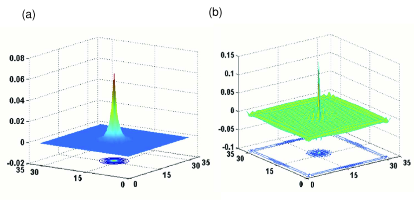
Figure 2: (Color online) (a) Charge density distribution (with the uniform background charge density distribution subtracted) for $n$=$1$, $\mu$=$0$ and at half filling case with two zero modes occupied. The charge (the integral of the charge density) is equal to $\frac{1}{2}e$. Here we give one layer case, and the other layer has the same distribution. (b) The axial charge density distribution with $n$=$1$ and $\mu$=$-$0.3. In all cases, we set the lattice system size as $N$=$32\mathtt{\times}32\mathtt{\times}2$, $h$=$0$, and $U$=$4$.

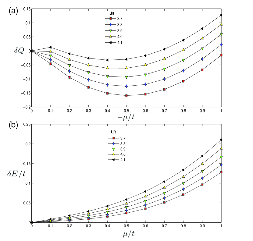
Figure 3: (Color online) (a) The axial charge bound to a vortex profile as a function of $U$ and $-\mu$. (b) Energy splitting [$E(N/2$+$1)-E(N/2)$] changes as a function of $U$ and $-\mu$. In both cases, $h$=$0$ and the vortex profile has vorticity $n$=$1$.

Numerics We perform exact diagonalization of the mean-field Hamiltonian of our system with $32\mathtt{\times}32$ sites per layer for symmetric vortex profile of the OP in quantum limit with the amplitude of OP calculated from the self-consistent solution of the BdG equations. In Fig. 2 we show the charge density distribution [Fig. 2(a)] and the axial charge [Fig. 2(b)] defined by $\delta Q_{\nu}$=$\sum_{i}[\left\langle\delta n_{i}\right\rangle_{\nu}\mathtt{-}\left\langle\delta n_{i}\right\rangle_{0}]$, with subscript $\nu(0)$ referring to the system with $1(0)$ vortex and $\delta n_{i}$=$n_{i2}\mathtt{-}n_{i1}$ the difference in the occupation number of the two layers.

The numeric results show the rational charge factionalization for $\mu$=$0$ and irrational fractional axial charge for $\mu\mathtt{\neq}0$. Here the rational fractional charge is exactly $\pm e/2$, independent of $U$. The dependence of $\delta Q_{\nu}$ on $\mu$ and $U$ in Fig. 3 (a) shows that the axial charge may be continuously tuned by changing the external parameters.

The splitting of the zero energy levels due to inter-valley interaction is shown in Fig. 3(b). The absence of splitting of zero energy levels for $\mu$=$0$ can also be understood from a perturbative analysis. It can be seen that the energy splitting has the form $\delta E\mathtt{\propto}|m_{0}\int e^{-i(\mathbf{K}_{+}-\mathbf{K}_{-})\cdot\mathbf{{r}}}$Re$[e^{-i\theta}(f^{2}$+$g^{2})]d\mathbf{r}|$. One can see that $\delta E$=$0$ with the help of solutions of Eqs. (14) and (16). Therefore, the inter-valley coupling does not split the degenerate zero modes. The existence of the exact zero modes ensures the charge fractionalization (per layer) as seen in Fig. 2 (a).

Discussions We propose a system of bilayer 2DEG adjacent to a type-II superconductor thin film for EC. The vortex profile for OP can be generated by defects or additional nontrivial texture in magnetic field jog . Furthermore, in our bilayer system, if a vacancy lies on a site in one layer and meanwhile an interstitial induced by impurities occurs at the underlying site in another layer, the nontrivial exciton OP with vortex profile is generated due to its minimal coupling to the nonzero axial gauge field emerged from the vacancy and interstitial relative to the magnetic flux lattices background. Moveover, the axial fractional charge bounding a magnetic flux quanta can form charge-flux composite particles which behave as Abelian anyons with the exchange phase $\gamma$=$\pi\delta Q_{\nu}$ under the standard argument Wick . Note that the above studies have ignored the intralayer next-nearest-neighbor hopping $t_{1}$ which may be important in the similar systems Rosen ; Hao , where the fractional charge is related to topologically nontrivial gapless edge states. However, the charge factionalization discussed in the present paper is different from that case, since the inter-layer interaction destroys the gapless edge states. Besides, unlike the crude crystalloid, the influence of $t_{1}$ here can be negligibly small since the lattice distance of the Abrikosov vortex square array can be adjusted very large.

The bilayer EC is analogous to the superconductor by the particle-hole transformation. That is why the BdG equations were used. Furthermore, many phenomena in superconductor have counterparts in bilayer EC, e.g., the vacancy induced suppression of the amplitude of the OP salk .

In summary, we have studied EC in a bilayer system which is likely to be fabricated in laboratory. In the presence of topological non-trivial OP profiles (vortex profiles), we have shown that the system exhibits rational/irrational fractional (axial) charge.

Acknowledgments This work was supported by NSFC under Grants No. 90921003, No. 10874020, No. 10574150 and No. 60776063, by the National Basic Research Program of China (973 Program) under Grants No. 2009CB929103, and by a grant of the China Academy of Engineering and Physics.

References

- (1) F. Wilczek, Phys. Rev. Lett. 48, 1144 (1982), 49, 957 (1982).
- (2) A.Kitaev, Ann. Phys. (N.Y.) 303, 2 (2003).
- (3) S. Das Sarma, C. Nayak and S. Tewari, Phys. Rev. B 73, 220502(R) (2006).
- (4) S. Tewari, S. Das Sarma, C. Nayak, C. W. Zhang and P. Zoller, Phys. Rev. Lett. 98, 010506 (2007).
- (5) N. Read and D. Green, Phys. Rev. B 61, 10267 (2000).
- (6) C.-Y. Hou, C. Chamon, and C. Mudry, Phys. Rev. Lett. 98, 186809 (2007).
- (7) B. Seradjeh, C. Weeks, and M. Franz Phys. Rev. B 77, 033104 (2008).
- (8) R. Jackiw and C. Rebbi, Phys. Rev. D 13, 3398 (1976).
- (9) C. Chamon, C.-Y. Hou, R. Jackiw, C. Mudry, S.-Y. Pi and G. Semenoff, Phys. Rev. B 77, 235431 (2008).
- (10) C. Weeks, G. Rosenberg, B. Seradjeh, and M. Franz, Nat. Phys. 3, 796 (2007).
- (11) T. Fukuzawa, E. E. Mendez and J. M. Hong Phys. Rev. Lett 64, 3066 (1990); L.V. Butov, A. Zrenner, G. Abstreiter, G. Böhm and G. Weimann, Phys. Rev. Lett 73, 304 (1994).
- (12) J. P. Eisenstein and A. H. MacDonald, Nature (London) 432, 691 (2004).
- (13) B. Seradjeh, H. Weber and M. Franz, Phys. Rev. Lett. 101, 246404 (2008).
- (14) A. I. Larkin and Yu. N. Ovchinnikov, Zh. Eksp. Tero. Fiz. 47, 1136 (1964) [Sov. Phys. JETP 20, 762 (1969)].
- (15) W.P. Su, J.R. Schrieffer, and A.J. Heeger, Phys. Rev. Lett. 42, 1698 (1979).
- (16) J. Goldstone and F. Wilczek, Phys. Rev. Lett. 47, 986 (1981).
- (17) E. J. Weinberg, Phys. Rev. D 24, 2669 (1981).
- (18) V. Gurarie and L. Radzihovsky, Phys. Rev. B 75, 212509 (2007).
- (19) A. V. Balatsky, Y. N. Joglekar, and P. B. Littlewood, Phys. Rev. Lett. 93, 266801 (2004).
- (20) F. Wilczek, Fractional Statistics and Anyon Superconductivity (World Scientific, Singapore, 1990).
- (21) G. Rosenberg, B. Seradjeh, C. Weeks and M. Franz, Phys. Rev. B 79, 205102 (2009).
- (22) N. Hao, W. Zhang, Z. Wang, Y. Wang, and P. Zhang, Phys. Rev. B 81, 125301 (2010).
- (23) M.I. Salkola, A.V. Balatsky, J. R. Schrieffer, Phys. Rev. B 55, 12648 (1997).