Kohn Anomaly in Raman Spectroscopy of Single Wall Carbon Nanotubes

Abstract

Phonon softening phenomena of the $\Gamma$ point optical modes including the longitudinal optical mode, transverse optical mode and radial breathing mode in “metallic” single wall carbon nanotubes are reviewed from a theoretical point of view. The effect of the curvature-induced mini-energy gap on the phonon softening which depends on the Fermi energy and chirality of the nanotube is the main subject of this article. We adopt an effective-mass model with a deformation-induced gauge field which provides us with a unified way to discuss the curvature effect and the electron-phonon interaction.

1 Introduction

The lattice structure of a single wall carbon nanotube (SWNT) can be specified uniquely by the chirality defined by two integers $(n,m)$ [Saito et al. (1992a, b)], and the chirality can be determined by Raman spectroscopy [Jorio et al. (2001, 2003); Dresselhaus et al. (2005)]. A simple tight-binding model shows that a SWNT is primarily metallic if $n-m$ is a multiple of 3 or semiconducting otherwise. A “metallic” SWNT can have a mini-energy band gap due to the curvature of a SWNT which gives rise to a hybridization between the $\sigma$ and $\pi$ orbitals. The presence of an energy band gap in a metallic SWNT has attracted much attention since the early stages of nanotube research [Hamada et al. (1992); Mintmire et al. (1992)]. The present paper deals with the effect of curvature on the Raman spectra for two in-plane $\Gamma$ point longitudinal and transverse optical phonon (LO and TO) modes [Farhat et al. (2007); Sasaki et al. (2008b)] and the out-of-plane radial breathing mode (RBM) [Farhat et al. (2009); Sasaki et al. (2008a)].

In the Raman spectra of a SWNT, the LO and TO phonon modes at the $\Gamma$ point in the two-dimensional Brillouin zone (2D BZ), which are degenerate in graphite and graphene, split into two peaks, denoted by $G^{+}$ and $G^{-}$ peaks, respectively, [Jorio et al. (2003); Saito et al. (1998, 2003)] because of the curvature effect. The splitting of the two peaks for SWNTs is inversely proportional to the square of the diameter, $d_{t}$, of SWNTs due to the curvature effect, in which $G^{+}$ does not change with changing $d_{t}$, but the $G^{-}$ frequency decreases with decreasing $d_{t}$ [Jorio et al. (2002)]. In particular, for metallic SWNTs, the $G^{-}$ peaks appear at a lower frequency than the $G^{-}$ peaks for semiconducting SWNTs with a similar diameter [Pimenta et al. (1998)]. The spectra of $G^{-}$ for metallic SWNTs show a much larger spectral width than that for semiconducting SWNTs.

It has been widely accepted that the frequency shift of the $G$-band in metallic SWNTs is produced by the electron-phonon (el-ph) interaction [Piscanec et al. (2004); Lazzeri and Mauri (2006); Ishikawa and Ando (2006); Popov and Lambin (2006); Caudal et al. (2007); Das et al. (2007)]. An optical phonon changes into an electron-hole pair as an intermediate state by the el-ph interaction. This process is responsible for the phonon self-energy. The phonon self-energy is sensitive to the structure of the Fermi surface [Kohn (1959)] or the Fermi energy, $E_{\rm F}$. In the case of graphite intercalation compounds in which the charge transfer of an electron from a dopant to the graphite layer can be controlled by the doping atom and its concentration, Eklund et al. (1977) observed a shift of the $G$-band frequency with an increase of the spectral width. In this case the frequency shifted spectra show that not only the LO mode but also the TO mode is shifted in the same fashion by a dopant. For a graphene mono-layer, Lazzeri et al. calculated the $E_{\rm F}$ dependence of the shift of the $G$-band frequency [Lazzeri and Mauri (2006)]. The LO mode softening in metallic SWNTs was shown by  Dubay et al. (2002); Dubay and Kresse (2003) on the basis of density functional theory. Recently Nguyen et al. (2007) and Farhat et al. (2007) observed the phonon softening effect of SWNTs experimentally as a function of $E_{\rm F}$ by electro-chemical doping, and their results clearly show that the LO phonon modes become soft as a function of $E_{\rm F}$. Ando (2008) discussed the phonon softening for metallic SWNTs as a function of the $E_{\rm F}$ position, in which the phonon softening occurs for the LO phonon mode. In this paper, we consider the effect of a curvature-induced mini-energy gap on the frequency of the LO, TO, and RBM in “metallic” SWNTs.

The organization of the paper is as follows. In Sec. 2 we show that the curvature of a SWNT gives rise to a hybridization between the $\sigma$ and $\pi$ orbitals. Then we show our calculated result for the curvature-induced mini-energy gap appearing in “metallic” SWNTs. The current status of the scanning tunneling spectroscopy experimental results is briefly mentioned, confirming the curvature-induced mini-energy gap. In Sec. 3 we formulate the phonon self-energy which is given by the electron-hole pair creation process. The Fermi energy dependence of the self-energy is shown for graphene with or without an energy gap, as a simple example. In Sec. 4 we provide a theoretical framework for including a lattice deformation into an effective-mass Hamiltonian. A lattice deformation is represented by a deformation-induced gauge field which is shown to be a useful idea to discuss both the appearance of the curvature-induced mini-energy gap and also the el-ph interaction. Sec. 5 is a main section in this article in which we discuss the effect of curvature on the phonon self energy. In Sec. 6 we discuss and summarize our results.

2 Curvature Effect

Let us start to discuss the effect of the curvature of a SWNT on the hybridization between the $\sigma$ and $\pi$ orbitals (Sec. 2.1), and we then show the calculated result of the curvature-induced mini-energy gap appearing in “metallic” SWNTs (Sec. 2.2). The phonon softening phenomena are sensitive to this mini-energy gap.

2.1 Curvature-Induced Hybridization

At each carbon atom located at ${\bf r}$ on the surface of a SWNT, we define the atom-specific $(x,y,z)$-coordinate axes and the unit vector for each axis by ${\bf e}_{i}({\bf r})$ ($i\in\{x,y,z\}$), where ${\bf e}_{z}({\bf r})$ is taken as the unit normal vector to the cylindrical surface, and ${\bf e}_{x}({\bf r})$ and ${\bf e}_{y}({\bf r})$ are unit vectors in the tangent plane [see Fig. 1(a)]. Here, ${\bf e}_{x}({\bf r})$ is taken to be parallel to the axis of a SWNT. In the case of a flat graphene sheet, we can set the common axis vector for all carbon atoms and thus a unit vector ${\bf e}_{i}$ at ${\bf r}_{1}$ can be taken orthogonal to the other ${\bf e}_{j}$ at ${\bf r}_{2}$ so that ${\bf e}_{i}({\bf r}_{1})\cdot{\bf e}_{j}({\bf r}_{2})=\delta_{ij}$. For SWNTs, however the orthogonal conditions are not satisfied because of the atom specific coordinate, that is, ${\bf e}_{z}({\bf r}_{1})\cdot{\bf e}_{z}({\bf r}_{2})\neq 1$, ${\bf e}_{z}({\bf r}_{1})\cdot{\bf e}_{y}({\bf r}_{2})\neq 0$, etc.

To see the curvature effect more clearly, it is useful to project ${\bf e}_{i}({\bf r}_{1})$ and ${\bf e}_{j}({\bf r}_{2})$ into

$${\bf e}_{i}({\bf r}_{1})={\bf e}_{i}^{\perp}({\bf r}_{1})+{\bf e}_{i}^{\parallel}({\bf r}_{1}),\ \ {\bf e}_{j}({\bf r}_{2})={\bf e}_{j}^{\perp}({\bf r}_{2})+{\bf e}_{j}^{\parallel}({\bf r}_{2}),$$ (1)

where $\parallel$ ($\perp$) denotes the vector which is parallel (perpendicular) to the displacement vector ${\bf r}_{2}-{\bf r}_{1}$ [see Fig. 1(b)]. Let $|p_{i}({\bf r})\rangle$ ($i\in\{x,y,z\}$) be the $2p_{i}$-orbital of a carbon atom located at ${\bf r}$. Then, the transfer integral from $|p_{i}({\bf r}_{1})\rangle$ to $|p_{j}({\bf r}_{2})\rangle$ may be written as

$$\langle p_{j}({\bf r}_{2})|{\hat{\cal H}}|p_{i}({\bf r}_{1})\rangle={\cal H}_{pp\pi}{\bf e}_{j}^{\perp}({\bf r}_{2})\cdot{\bf e}_{i}^{\perp}({\bf r}_{1})+{\cal H}_{pp\sigma}{\bf e}_{j}^{\parallel}({\bf r}_{2})\cdot{\bf e}_{i}^{\parallel}({\bf r}_{1}),$$ (2)

where ${\cal H}_{pp\pi}$ and ${\cal H}_{pp\sigma}$ are the transfer integrals for $\pi$ and $\sigma$ bonds, respectively. According to a first-principles calculation with the local density approximation obtained by Porezag et al. (1995), ${\cal H}_{pp\pi}\approx-3$ eV and ${\cal H}_{pp\sigma}\approx 8$ eV for nearest-neighbor carbon sites. Using Eq. (1), we eliminate ${\bf e}_{i}^{\perp}({\bf r}_{1})$ and ${\bf e}_{j}^{\perp}({\bf r}_{2})$ from Eq. (2), and get

$$\langle p_{j}({\bf r}_{2})|{\hat{\cal H}}|p_{i}({\bf r}_{1})\rangle={\cal H}_{pp\pi}{\bf e}_{j}({\bf r}_{2})\cdot{\bf e}_{i}({\bf r}_{1})+\left({\cal H}_{pp\sigma}-{\cal H}_{pp\pi}\right){\bf e}_{j}^{\parallel}({\bf r}_{2})\cdot{\bf e}_{i}^{\parallel}({\bf r}_{1}),$$ (3)

where we have used ${\bf e}_{i}^{\perp}({\bf r}_{1})\cdot{\bf e}_{j}^{\parallel}({\bf r}_{2})=0$ and ${\bf e}_{i}^{\parallel}({\bf r}_{1})\cdot{\bf e}_{j}^{\perp}({\bf r}_{2})=0$. The last term of Eq. (3) corresponds to the curvature effect of a SWNT. Note that the coefficient of the last term includes ${\cal H}_{pp\sigma}$ showing that the $\sigma$ bond is partially incorporated by the curvature-induced hybridization [See Ando (2000) for more details].

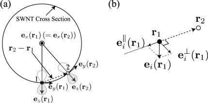
Figure 1: (a) The curvature-induced hybridization between two $p_{z}$ orbitals of carbon atoms at ${\bf r}_{1}$ and ${\bf r}_{2}$ is illustrated. ${\bf e}_{i}({\bf r})$ ($i\in\{x,y,z\}$) denotes the basis of the $(x,y,z)$-coordinate system whose origin is located at a carbon atom ${\bf r}$. (b) ${\bf e}_{i}^{\parallel}({\bf r}_{2})$ and ${\bf e}_{i}^{\parallel}({\bf r}_{1})$ induce the hybridization, including $\sigma$ bonding.

In the case of a flat graphene, we have ${\bf e}_{z}^{\parallel}({\bf r}_{1})=0$ and ${\bf e}_{z}^{\parallel}({\bf r}_{2})=0$. Then, the last term of Eq. (3) disappears and the theoretical model taking only the $2p_{z}$ orbital (or $\pi$-orbital) into account becomes a good approximation. The curvature of a SWNT results in ${\bf e}_{z}^{\parallel}({\bf r}_{2})\cdot{\bf e}_{z}^{\parallel}({\bf r}_{1})\neq 0$, ${\bf e}_{z}^{\parallel}({\bf r}_{2})\cdot{\bf e}_{y}^{\parallel}({\bf r}_{1})\neq 0$, etc., and the last term of Eq. (3) is non-vanishing and consequently the curvature-induced hybridization occurs. The curvature-induced hybridization is relevant to the following two physical properties. First, the hybridization can open a mini-gap (up to $\sim$ 100meV) near the Fermi energy in metallic SWNTs. Second, the curvature-induced gap depends on the SWNT $(n,m)$ chirality. For example, the gap is zero for armchair SWNTs, while it is about 70 meV for a $(12,0)$ metallic zigzag SWNT. The chirality dependent curvature-induced energy gap will be analytically given in the next subsection.

2.2 Curvature-Induced Mini-Energy Gap

In Fig. 2(a) we plot the calculated curvature-induced energy gap, $E_{\rm gap}$, for each $(n,m)$ for metallic SWNTs as a function of the chiral angle $\theta(^{\circ})$ and tube diameter $d_{t}$(nm). We performed the energy band structure calculation in an extended tight-binding (ETB) framework developed by Samsonidze et al. (2004) to obtain $E_{\rm gap}$. In the ETB framework, $2s$ and $2p$ orbitals, and their transfer and overlap integrals up to fourth nearest neighbor atoms are taken into account [see Popov (2004); Samsonidze et al. (2004) for more details].  We have adopted the values of the transfer and overlap integrals as a function of the carbon-carbon inter-atomic distance that were derived by Porezag et al. (1995). 

Figure 2(a) shows that, for a fixed diameter of a metallic SWNT $d_{t}$, a zigzag SWNT ($\theta=0^{\circ}$) has the largest value of $E_{\rm gap}$ and an armchair SWNT ($\theta=30^{\circ}$) has no energy gap. The calculated results are well reproduced by

$$E_{\rm gap}=\frac{c}{d_{t}^{2}}\cos 3\theta,$$ (4)

with $c=60$(eV$\cdot$nm²) [Sasaki et al. (2008a)]. The chirality and diameter dependence of $E_{\rm gap}$ is consistent with the results by Kane and Mele (1997), and Ando (2000). The value of $c$ is about two times larger than the result by Kane and Mele (1997). This difference may come from the inclusion of ${\cal H}_{pp\sigma}$ in our calculation. As we will explain in detail in Sec. 4.2, the curvature moves the Dirac point in $k$-space away from the hexagonal corner of the first BZ. As a result, the curvature can cause the quantized transverse electron wave vector (the cutting line) to miss the Dirac point and make a gap [see the inset in Fig. 2(a)].

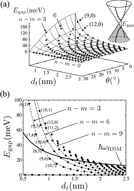
Figure 2: (a) The dependence of the curvature-induced energy gap, $E_{\rm gap}$, on the chiral angle $\theta$ and tube diameter $d_{t}$. The surface is a plot of Eq. (4) which reproduces well the calculated results. (inset) Due to the nanotube curvature, the cutting line which was exactly crossing the Dirac point in the absence of curvature can miss the Dirac point when curvature is included. This curvature gives rise to an energy gap $E_{\rm gap}$ in “metallic” SWNTs. (b) The $d_{t}$ dependence of $E_{\rm gap}$ is given as a one-dimensional projection of (a) onto the $d_{t}$ axis. The points on the dashed, dot-dashed, and dotted curves satisfy $n-m=3,6,9$, respectively. We plot the energy of the RBM, $\hbar\omega_{\rm RBM}$ of Eq. (5), as a solid curve for comparison.

When we discuss the phonon softening of the RBM, the relationship between the mini-energy gap and the RBM phonon energy will be important. In Fig. 2(b), we plot the energy of the RBM,

$$\hbar\omega_{\rm RBM}=\frac{c_{1}}{d_{t}}+c_{2},$$ (5)

as a solid curve for comparison. Here $\hbar\omega_{\rm RBM}$ is a monotonic function of the tube diameter ($d_{t}$[nm]) and is modeled as being linear in the inverse diameter, with an offset $c_{2}$ which is known as the effect of the substrate. We assume that $c_{1}=223.5$[cm^-1] and $c_{2}=12.5$[cm^-1] which are experimentally derived parameters as obtained by Strano et al. (2003) and Bachilo et al. (2002). Using Eqs. (5) and (4) for zigzag SWNTs ($\theta=0^{\circ}$), we see that $E_{\rm gap}$ is smaller than $\hbar\omega_{\rm RBM}$ when $d_{t}>2$[nm] (see Fig. 2(b)).

The presence (absence) of a curvature-induced mini-energy gap in “metallic” zigzag (armchair) SWNTs was confirmed experimentally by Ouyang et al. (2001). The chirality was measured experimentally for $(9,0)$, $(12,0)$, and $(15,0)$ zigzag SWNTs by these authors. The observed energy gap can be fitted by $4A_{0}/d_{t}^{2}$ which has the same $d_{t}$ dependence in Eq. (4). Note that the coefficient is given by $A_{0}=3\gamma_{0}a_{\rm cc}^{2}/16$, and $4A_{0}\approx 40$[meV$\cdot$nm²] is smaller than the value of $c=60$[meV$\cdot$nm²] in Eq. (4).  This discrepancy may be attributed to (1) uniaxial and torsional strain which is unintentionally applied to a SWNT [Yang et al. (1999); Yang and Han (2000); Kleiner and Eggert (2001)],  or (2) renormalization of the value of $c$ due to the el-ph interaction, or (3) a SWNT-substrate interaction effect. (1,2) are intrinsic to SWNTs, while (3) is extrinsic. Since there are various factors which can affect the energy gap, it is not easy to predict the precise value of the energy gap, although the curvature-induced gap has been examined within the framework of first principles calculations including the effect of structure optimization [Miyake and Saito (2005)]. It is noted that the chirality dependence of $\cos 3\theta$ in Eq. (4) has not been tested experimentally so far, except for $\theta=0$ (zigzag SWNTs) and $\theta=30^{\circ}$ (armchair SWNTs). Study of a chiral SWNT is left for future experiments.

3 Effect of Curvature on the Phonon Energy

In this section we formulate the self-energy of a phonon mode (Sec. 3.1), and explain qualitatively the effect of the curvature on the self-energy (Sec. 3.2). The relationship between our formulation and that of others is referred to in Sec. 3.3.

3.1 Phonon Self-Energy

A renormalized phonon energy is written as a sum of the unrenormalized energy, $\hbar\omega$, and the real part of the self-energy, $\Pi(\omega,E_{\rm F})$. The imaginary part of $\Pi(\omega,E_{\rm F})$ gives the spectrum width. Throughout this paper, we assume a constant value for $\hbar\omega$ for each phonon mode. The self-energy is given by time-dependent second-order perturbation theory as

$$\Pi(\omega,E_{\rm F})=2\sum_{\bf k}\left(\frac{|V_{\bf k}|^{2}}{\hbar\omega-E^{\rm eh}_{\bf k}+i\Gamma/2}-\frac{|V_{\bf k}|^{2}}{\hbar\omega+E^{\rm eh}_{\bf k}+i\Gamma/2}\right)\times\left(f_{\rm h}-f_{\rm e}\right),$$ (7)

where the pre-factor 2 comes from spin degeneracy, $f_{\rm h,e}=(1+\exp(\beta(E^{\rm h,e}-E_{\rm F}))^{-1}$ is the Fermi distribution function, $E^{\rm e}_{\bf k}$ ($E^{\rm h}_{\bf k}$) is the energy of an electron (a hole) with momentum ${\bf k}$, and $E^{\rm eh}_{\bf k}\equiv E^{\rm e}_{\bf k}-E^{\rm h}_{\bf k}$ ($\geq 0$) is the energy of an electron-hole pair. $V_{\bf k}$ is the el-ph matrix element that a phonon with momentum ${\bf q}=0$ changes into an electron-hole pair [see the left diagram of Fig. 3(a)] which will be derived in Sec. 4. Note that the momentum of an electron ${\bf k}$ is the same as that of a hole due to momentum conservation, and therefore pair creation involves a vertical transition. In Eq. (7), the energy shift is given by the real part of the self-energy, ${\rm Re}[\Pi(\omega,E_{\rm F})]$, and the decay width $\Gamma$ is determined self-consistently by $\Gamma/2=-{\rm Im}\left[\Pi(\omega,E_{\rm F})\right]$.  The decay width relates to the average life-time $\tau$ via $\tau=\hbar/\Gamma$. It is noted that we use $T=300$K although the self-energy is also a function of temperature [$\beta^{-1}=k_{\rm B}T$ where $k_{\rm B}$ is Boltzmann’s constant].

3.2 Phonon Softening and Hardening

By defining the denominators of Eq. (7) as $h_{\pm}(E^{\rm eh})\equiv\pm 1/(\hbar\omega\mp E^{\rm eh}+i\Gamma/2)$, Eq. (7) may be rewritten as

$$\Pi(\omega,E_{\rm F})=2\sum_{\bf k}|V_{\bf k}|^{2}\left[h_{+}(E^{\rm eh}_{\bf k})+h_{-}(E^{\rm eh}_{\bf k})\right]\times\left(f_{\rm h}-f_{\rm e}\right).$$ (8)

When we assume that $|V_{\bf k}|^{2}$ does not depend on ${\bf k}$, the $E^{\rm eh}$ dependence of ${\rm Re}[\Pi(\omega,E^{\rm eh})]$ is determined by those of ${\rm Re}[h_{+}(E^{\rm eh})]$ and ${\rm Re}[h_{-}(E^{\rm eh})]$. It should be noted that ${\rm Re}[h_{+}(E^{\rm eh})]$ (solid curve in Fig. 3(b)) has a positive (negative) value when $E^{\rm eh}<\hbar\omega$ ($E^{\rm eh}>\hbar\omega$), and the lower (higher) energy electron-hole pair makes a positive (negative) contribution to ${\rm Re}[\Pi(\omega,E_{\rm F})]$. Therefore, the sign of the contribution to ${\rm Re}[\Pi(\omega,E_{\rm F})]$, i.e., frequency hardening or softening, depends on its electron-hole virtual state energy, $E^{\rm eh}$. In contrast, ${\rm Re}[h_{-}(E^{\rm eh})]$ (dashed curve in Fig. 3(b)) always has a negative value, that is, it only contributes to a phonon softening. Note however that the contribution of ${\rm Re}[h_{-}(E^{\rm eh})]$ is small compared with ${\rm Re}[h_{+}(E^{\rm eh})]$ since $-1/\hbar\omega\leq{\rm Re}[h_{-}(E^{\rm eh})]<0$. Physically speaking, the $h_{-}(E^{\rm eh})$ term represents an intermediate state including two phonons and electron-hole pairs (see the right hand diagram in Fig. 3(a)), while the $h_{+}(E^{\rm eh})$ term represents the intermediate state that includes only electron-hole pairs.  Even though the contribution of $h_{-}(E^{\rm eh})$ is relatively small, $h_{-}(E^{\rm eh})$ is important to get a symmetric response of $\Pi(\omega,E_{\rm F})$ relative to the Fermi energy. In fact, due to the $h_{-}(E^{\rm eh})$ term, the electron-hole pair at the Dirac point ($E^{\rm eh}=0$) can not contribute to the self-energy, since ${\rm Re}[h_{+}(E^{\rm eh})+h_{-}(E^{\rm eh})]=0$ when $E^{\rm eh}=0$. For high energy electron-hole pairs, the $h_{\pm}(E^{\rm eh})$ terms contribute equally since ${\rm Re}[h_{+}(E^{\rm eh})]\approx{\rm Re}[h_{-}(E^{\rm eh})]\approx-1/E^{\rm eh}$.

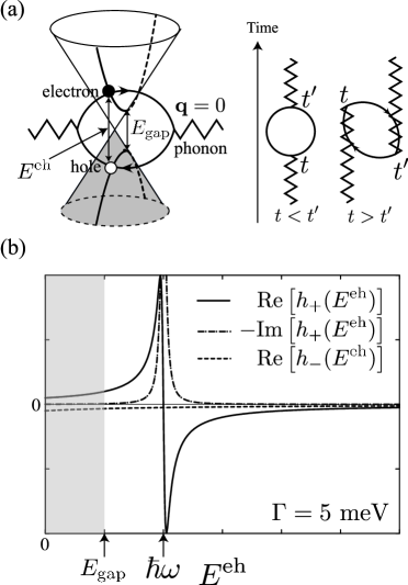
Figure 3: (a) In time-dependent second-order perturbation theory, we consider an intermediate state including only electron-hole pairs (the case of $t<t^{\prime}$), and an intermediate state including two phonons and electron-hole pairs (the case of $t>t^{\prime}$). The former process corresponds to $h_{+}(E^{\rm eh})$, while the latter one corresponds to $h_{-}(E^{\rm eh})$. (b) The energy correction to the phonon energy by an intermediate electron-hole pair, especially the sign of ${\rm Re}(h_{+}(E^{\rm eh}))$ (solid curve), that corresponds to frequency hardening or softening, depends on the energy of the intermediate state $E^{\rm eh}$. The contribution to $\Pi(\omega,E_{\rm F})$ of a low energy electron-hole pair satisfying $0\leq E^{\rm eh}\leq E_{\rm gap}$ is forbidden. ${\rm Im}(h_{+}(E^{\rm eh}))$ (dashed curve) is nonzero only when $E^{\rm eh}$ is very close to $\hbar\omega$, which shows that a phonon mode can resonantly decay into an electron-hole pair with the same energy.

The curvature-induced energy gap, $E_{\rm gap}$, affects the frequency shift since an electron-hole pair creation event is possible only when $E^{\rm eh}\geq E_{\rm gap}$. When $0<E_{\rm gap}\leq\hbar\omega$, the contribution to frequency hardening in Eq. (7) is suppressed. When $E_{\rm gap}>\hbar\omega$, not only are all the positive contributions to the self-energy suppressed, but some negative contributions are also suppressed. Further, ${\rm Im}(h_{+}(E^{\rm eh}))$ is nonzero only when $E^{\rm eh}$ is very close to $\hbar\omega$, which shows that a phonon can resonantly decay into an electron-hole pair with the same energy. Thus, when $E_{\rm gap}>\hbar\omega$, we have $\Gamma\simeq 0$ because no resonant electron-hole pair excitation is allowed near $E=\hbar\omega$. It is therefore important to compare the values of $E_{\rm gap}$ and $\hbar\omega$ for each $(n,m)$ SWNT. For the LO and TO modes, $\hbar\omega$ is about 0.2[eV] and therefore we get $E_{\rm gap}<\hbar\omega$ (see Fig. 2) for most of the SWNTs except for a SWNT with a small diameter.  Thus, those LO and TO modes can resonantly decay into an electron-hole pair. The RBM mode in some SWNTs (for example, a $(12,0)$ zigzag SWNT) can not resonantly decay into an electron-hole pair, which results in a long life-time for the RBM in that particular SWNT [Sasaki et al. (2008a)].

At $T=0$, the Fermi distribution factor, namely $f_{\rm h}-f_{\rm e}$ in Eq. (7), plays a very similar role as the curvature-induced gap, $E_{\rm gap}$. In fact, all the excitations of electron-hole pairs with $E^{\rm eh}\leq 2|E_{\rm F}|$ are forbidden due to the Pauli exclusion principle. A difference between the energy gap and the Fermi energy arises at a finite temperature. Some electron-hole pairs with $E_{\rm gap}\leq E^{\rm eh}\leq 2|E_{\rm F}|$ can contribute to the self-energy, while states $E^{\rm eh}<E_{\rm gap}$ do not exist even at a finite temperature. It should be noted that $V_{\bf k}$ in Eq. (7) depends on the value of $E_{\rm gap}$ since the position of the cutting line depends on $E_{\rm gap}$, while $V_{\bf k}$ does not change by changing $E_{\rm F}$. This is also a crucial difference between the roles of $E_{\rm gap}$ and $E_{\rm F}$ in the self-energy.

3.3 Other Formulas

Here, we refer to the relationship between our formula and other formulas. First, replacing $\Gamma/2$ in Eq. (7) with a positive infinitesimal $0_{+}$ gives the standard formula for the Fermi Golden rule. In this case, using $1/(x+i0_{+})={\rm P}(1/x)-i\pi\delta(x)$ with ${\rm P}$ denoting the principle value of integration and $\delta(x)$ the Dirac delta-function, $\Gamma/2$ can be calculated directly, i.e., without using the self-consistent way, by performing the summation (or integral) of the right-hand side of Eq. (7). We calculate $\Gamma/2$ self-consistently by taking care of a finite energy level spacing originating from a finite length of a nanotube where $E^{\rm eh}_{\bf k}$ now takes a discrete value, and is not a continuous variable. Roughly speaking, the broadening is suppressed when the energy level spacing, $\Delta E=2\pi\hbar v_{\rm F}/L$, exceeds $\Gamma$. For example, the critical length where the broadening becomes negligible for a $(10,10)$ SWNT is about $700$nm.

Second, the summation index $\sum_{\bf k}$ in Eq. (7) is not restricted to only inter-band ($E^{\rm eh}\neq 0$) processes but includes also intra-band ($E^{\rm eh}=0$) processes.  Then, the self-energy can be decomposed into two parts, as $\Pi(\omega,E_{\rm F})=\Pi^{\rm inter}(\omega,E_{\rm F})+\Pi^{\rm intra}(\omega,E_{\rm F})$ where $\Pi^{\rm inter}(\omega,E_{\rm F})$ includes only inter-band processes satisfying $E^{\rm eh}\neq 0$. In the adiabatic limit, i.e., when $\omega=0$ and $\Gamma=0$ in Eq. (7), it is straightforward to get the following relations, for a single Dirac cone at $T=0$:

$$\begin{split}&\Pi^{\rm intra}(0,E_{\rm F})=-2\sum_{\bf k}|V_{\bf k}|^{2}\times\begin{cases}f^{\prime}(E^{\rm e}_{\bf k}),(E_{\rm F}>0)\\ f^{\prime}(E^{\rm h}_{\bf k}),(E_{\rm F}<0)\end{cases}=-\frac{\alpha}{2}|E_{\rm F}|,\\ &\Pi^{\rm inter}(0,E_{\rm F})=-4\sum_{\bf k}\frac{|V_{\bf k}|^{2}}{E^{\rm eh}_{\bf k}}=-\frac{\alpha}{2}\left(E_{c}-|E_{\rm F}|\right),\end{split}$$ (9)

where $\alpha\equiv S|v|^{2}/\pi(\hbar v_{\rm F})^{2}$ and $E_{c}$ is some cut-off energy. Here, we have assumed that $V_{\bf k}=v\cos\Theta({\bf k})$.  Note that $\Pi^{\rm intra}(0,E_{\rm F})$ does not vanish because $(f_{\rm h}-f_{\rm e})/E^{\rm eh}_{\bf k}\neq 0$ in this limit, while in the non-adiabatic case, $\Pi^{\rm intra}(\omega,E_{\rm F})$ vanishes since $(f_{\rm h}-f_{\rm e})/\hbar\omega=0$. It is only the inter-band process that contributes to the self-energy in the non-adiabatic case.  In the non-adiabatic limit at $T=0$, it is a straightforward calculation to get

$${\rm Re}\left[\Pi(\omega,E_{\rm F})\right]=-\frac{\alpha}{2}\left[E_{c}-|E_{\rm F}|-\frac{\hbar\omega}{4}\ln\left|\frac{|E_{\rm F}|-\frac{\hbar\omega}{2}}{|E_{\rm F}|+\frac{\hbar\omega}{2}}\right|\right],\ \ (E_{c}\gg\hbar\omega),$$ (10)

where $E^{\rm eh}_{\bf k}=2\hbar v_{\rm F}k$, $\sum_{\bf k}\to V/(2\pi)^{2}\int_{0}^{k_{c}}kdk\int_{0}^{2\pi}d\Theta$, and $\int x/(x+a)dx=x-a\ln|x+a|$ have been used in Eq. (7) to get the right-hand side. The Fermi energy dependence is given by the last two terms for the case of a massless Dirac cone spectrum. The first term is linear with respect to $E_{\rm F}$ and the second term produces a singularity at $|E_{\rm F}|=\hbar\omega/2$. This singularity is useful in identifying the actual Fermi energy of a graphene sample.

It is also interesting to consider the case of a massive Dirac cone spectrum, $E=\pm\sqrt{m^{2}+(\hbar v_{\rm F}k)^{2}}$. In the non-adiabatic limit at $T=0$, we get

$${\rm Re}\left[\Pi(\omega,E_{\rm F})\right]=-\frac{\alpha}{2}\left[E_{c}-|E_{\rm F}|-\left\{\frac{\left(\hbar\omega\right)^{2}-(2m)^{2}}{4\hbar\omega}\right\}\ln\left|\frac{|E_{\rm F}|-\frac{\hbar\omega}{2}}{|E_{\rm F}|+\frac{\hbar\omega}{2}}\right|\right],$$ (11)

where $E_{c}\gg\hbar\omega$ and $V_{\bf k}=v(\hbar v_{\rm F}k/E)\cos\Theta({\bf k})$ are assumed. Equation (11) is for $|E_{\rm F}|\geq m$. For $|E_{\rm F}|<m$, the self-energy shift is given by replacing $|E_{\rm F}|$ with $m$ in Eq. (11). The logarithmic singularity for the last term disappears when $m=\hbar\omega/2$, and its overall sign is interchanged when $2m>\hbar\omega$. Broadening is possible only when $2m<\hbar\omega$, which may be useful in knowing whether the graphene sample has an energy gap or not.

4 The Electron-Phonon Interaction

In this section we provide a framework to obtain the el-ph (electron-phonon) interaction in the effective-mass theory, and show how to calculate the el-ph matrix elements. The main results are Eqs. (22) and (47). Those who are not interested in the details of the derivation can skip this section.

4.1 Unperturbed Hamiltonian

The unperturbed Hamiltonian in the effective-mass model for $\pi$-electrons near the K point of a graphene sheet is given by

$${\cal H}^{\rm K}_{0}=v_{\rm F}\mbox{\boldmath$\sigma$}\cdot\hat{\mathbf{p}},$$ (12)

where $v_{\rm F}$ is the Fermi velocity, $\hat{\bf p}=-i\hbar\nabla$ is the momentum operator, and $\mbox{\boldmath$\sigma$}=(\sigma_{x},\sigma_{y})$ is the Pauli matrix.  The $x$, $y$, and $z$ coordinate system is taken as shown in Fig. 4. ${\cal H}^{\rm K}_{0}$ is a $2\times 2$ matrix which operates on the two component wavefunction:

$$\psi^{\rm K}({\bf r})=\begin{pmatrix}\psi^{\rm K}_{\rm A}({\bf r})\cr\psi^{\rm K}_{\rm B}({\bf r})\end{pmatrix},$$ (13)

where $\psi^{\rm K}_{\rm A}({\bf r})$ and $\psi^{\rm K}_{\rm B}({\bf r})$ are the wavefunctions of $\pi$-electrons for the sublattices A and B, respectively, around the K point. The energy eigenvalue of Eq. (12) is given by $\pm v_{\rm F}|{\bf p}|$ and the energy dispersion relation shows a linear dependence at the Fermi point, which forms what is known as the Dirac cone.

The energy eigenstate with wave vector ${\bf k}$ in the conduction energy band is written by a plane wave $e^{i{\bf k}\cdot{\bf r}}$ with the Bloch function $\psi^{\rm K}_{{\rm c},{\bf k}}$ as $\psi^{\rm K}_{{\rm c},{\bf k}}({\bf r})=Ne^{i{\bf k}\cdot{\bf r}}\psi^{\rm K}_{{\rm c},{\bf k}}$ where $N$ is a normalization constant satisfying $N^{2}S=1$, $S$ is the area (volume) of the system, and

$$\psi^{\rm K}_{{\rm c},{\bf k}}\equiv\frac{1}{\sqrt{2}}\begin{pmatrix}1\cr e^{i\Theta({\bf k})}\end{pmatrix}.$$ (14)

Here ${\bf k}$ is measured from the K point, and $\Theta({\bf k})$ is defined by an angle of ${\bf k}=(k_{x},k_{y})$ measured from the $k_{x}$-axis as $(k_{x},k_{y})\equiv|{\bf k}|(\cos\Theta({\bf k}),\sin\Theta({\bf k}))$. The eigen value of this state is $E=+v_{\rm F}|{\bf p}|$. The energy eigenstate with the energy eigen value $E=-v_{\rm F}|{\bf p}|$ in the valence energy band is written by

$$\psi^{\rm K}_{v,{\bf k}}({\bf r})=\frac{e^{i{\bf k}\cdot{\bf r}}}{\sqrt{2S}}\begin{pmatrix}1\cr-e^{+i\Theta({\bf k})}\end{pmatrix}.$$ (15)

The energy eigenstate for the valence band, $\psi^{\rm K}_{v,{\bf k}}({\bf r})$ is given by $\sigma_{z}\psi^{\rm K}_{c,{\bf k}}({\bf r})$. This results from the particle-hole symmetry of the Hamiltonian: $\sigma_{z}{\cal H}^{\rm K}_{0}\sigma_{z}=-{\cal H}_{0}^{\rm K}$.

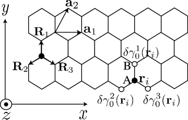
Figure 4: A hexagonal unit cell of graphene consists of A (closed circle) and B (open circle) sublattices. ${\bf a}_{1}$ and ${\bf a}_{2}$ are lattice vectors. ${\bf R}_{a}$ ($a=1,2,3$) are vectors pointing to the nearest-neighbor B sites from an A site (${\bf R}_{1}=a_{\rm cc}{\bf e}_{y}$, ${\bf R}_{2}=-(\sqrt{3}/2)a_{\rm cc}{\bf e}_{x}-(1/2)a_{\rm cc}{\bf e}_{y}$, and ${\bf R}_{3}=(\sqrt{3}/2)a_{\rm cc}{\bf e}_{x}-(1/2)a_{\rm cc}{\bf e}_{y}$) where ${\bf e}_{x}$ (${\bf e}_{y}$) is the dimensionless unit vector for the $x$-axis ($y$-axis). Local modulations of the hopping integral are defined by $\delta\gamma^{a}_{0}({\bf r}_{i})$ ($a=1,2,3$) where ${\bf r}_{i}$ is the position of an A-atom.

The unperturbed Hamiltonian near the K^′ point is given by

$${\cal H}^{\rm K^{\prime}}_{0}=v_{\rm F}\mbox{\boldmath$\sigma$}^{\prime}\cdot\hat{\mathbf{p}},$$ (16)

where $\mbox{\boldmath$\sigma$}^{\prime}=(-\sigma_{x},\sigma_{y})$. The dynamics of $\pi$-electrons near the K^′ point relates to the electrons near the K point by time-reversal symmetry, $\psi^{\rm K}\to(\psi^{\rm K^{\prime}})^{*}$ [Sasaki and Saito (2008)]. Because lattice vibrations do not break time-reversal symmetry, we mainly consider electrons near the K point in this paper.

4.2 Deformation-Induced Gauge Field

Lattice deformation modifies the nearest-neighbor hopping integral locally as $-\gamma_{0}\to-\gamma_{0}+\delta\gamma_{0}^{a}({\bf r}_{i})$ ($a=1,2,3$) (see Fig. 4). The corresponding perturbation of the lattice deformation is given by

$${\cal H}_{1}\equiv\sum_{i\in{\rm A}}\sum_{a=1,2,3}\delta\gamma^{a}_{0}(\mathbf{r}_{i})\left[(c_{i+a}^{\rm B})^{\dagger}c_{i}^{\rm A}+(c_{i}^{\rm A})^{\dagger}c_{i+a}^{\rm B}\right],$$ (17)

where $c_{i}^{\rm A}$ is the annihilation operator of a $\pi$ electron of an A-atom at position ${\bf r}_{i}$, and $(c^{\rm B}_{i+a})^{\dagger}$ is a creation operator at position ${\bf r}_{i+a}$ $(={\bf r}_{i}+{\bf R}_{a})$ of a B-atom where ${\bf R}_{a}$ ($a=1,2,3$) are vectors pointing to the three nearest-neighbor B sites from an A site.

The perturbation of Eq. (17) gives rise to scattering within a region near the K point (intravalley scattering) whose interaction is given by a deformation-induced gauge field ${\bf A}({\bf r})=(A_{x}({\bf r}),A_{y}({\bf r}))$ in Eq. (12) as

$${\cal H}^{\rm K}_{0}+{\cal H}^{\rm K}_{1}=v_{\rm F}\mbox{\boldmath$\sigma$}\cdot\left[\hat{\mathbf{p}}+{\bf A}^{\rm q}({\bf r})\right],$$ (18)

where ${\bf A}^{\rm q}({\bf r})$ is defined from $\delta\gamma_{0,a}({\bf r})$ ($a=1,2,3$) as [Sasaki et al. (2005, 2006); Katsnelson and Geim (2008)]

$$\begin{split}&v_{\rm F}A^{\rm q}_{x}({\bf r})=\delta\gamma_{0,1}({\bf r})-\frac{1}{2}\left[\delta\gamma_{0,2}({\bf r})+\delta\gamma_{0,3}({\bf r})\right],\\ &v_{\rm F}A^{\rm q}_{y}({\bf r})=\frac{\sqrt{3}}{2}\left[\delta\gamma_{0,2}({\bf r})-\delta\gamma_{0,3}({\bf r})\right].\end{split}$$ (19)

When $\delta\gamma_{0,2}=\delta\gamma_{0,3}=0$, then ${\bf A}^{\rm q}({\bf r})=(A_{x}({\bf r}),0)$ and ${\bf A}^{\rm q}({\bf r})\cdot{\bf R}_{1}=0$. Similarly, when $\delta\gamma_{0,1}=\delta\gamma_{0,3}=0$, we have ${\bf A}^{\rm q}({\bf r})\cdot{\bf R}_{2}=0$. Generally, the direction of ${\bf A}^{\rm q}({\bf r})$ is pointing perpendicular to the bond whose hopping integral is changed from $\gamma_{0}$. For the K^′ point, we obtain

$${\cal H}^{\rm K^{\prime}}_{0}+{\cal H}^{\rm K^{\prime}}_{1}=v_{\rm F}\mbox{\boldmath$\sigma$}^{\prime}\cdot\left[\hat{\mathbf{p}}-{\bf A}^{\rm q}({\bf r})\right].$$ (20)

Even though the ${\bf A}^{\rm q}({\bf r})$ appears as a gauge field, it does not break time-reversal symmetry because the sign in front of ${\bf A}^{\rm q}({\bf r})$ is opposite to each other for the K and K^′ points. This is in contrast with the fact that ${\bf A}({\bf r})$ (vector potential) violates time-reversal symmetry because the sign in front of ${\bf A}({\bf r})$ is the same for the K and K^′ points since ${\hat{\bf p}}\to{\hat{\bf p}}-e{\bf A}({\bf r})$ in the presence of a magnetic field.

The gauge field description for the lattice deformation (Eq. (19)) is useful to show the appearance of the curvature-induced mini-energy gap in metallic carbon nanotubes. For a zigzag nanotube, we have $\delta\gamma_{0,1}=0$ and $\delta\gamma_{0,2}=\delta\gamma_{0,3}\neq 0$ from the rotational symmetry around the tube axis (see Fig. 4). Then, Eq. (19) shows that for $A^{\rm q}_{x}\neq 0$ and $A^{\rm q}_{y}=0$, the cutting line of $k_{x}=0$ for the metallic zigzag nanotube is shifted by a finite constant value of $A^{\rm q}_{x}$ because of the Aharanov-Bohm effect for the lattice distortion-induced gauge field ${\bf A}^{\rm q}$. For an armchair nanotube, we have $\delta\gamma_{0,1}\neq 0$ and $\delta\gamma_{0,2}=\delta\gamma_{0,3}$. Then, Eq. (19) shows that for $A^{\rm q}_{x}\neq 0$ and $A^{\rm q}_{y}=0$, the cutting line of $k_{y}=0$ for the armchair nanotube is not shifted by a vanishing $A^{\rm q}_{y}$. This explains the presence (absence) of the curvature-induced mini-energy gap in metallic zigzag (armchair) carbon nanotubes [Kane and Mele (1997)].

The gauge field description is also useful to discuss the effect of an uniaxial strain on the gap. Let us consider applying a strain along the axis of a zigzag SWNT. Then, due to the symmetry, we have $\delta\gamma_{0,1}=a$ and $\delta\gamma_{0,2}=\delta\gamma_{0,3}=a/2$ where $a$ is a constant. Putting these perturbations into Eq. (19) we see that $v_{\rm F}A^{\rm q}_{x}=a/2$, which means that the curvature-induced gap in a zigzag nanotube can change a little by the strain along the axis. For an armchair SWNT, instead, we have $\delta\gamma_{0,1}=0$ and $\delta\gamma_{0,2}=\delta\gamma_{0,3}=b$, which results in $v_{\rm F}A^{\rm q}_{y}=0$. This shows that the absence of the gap in armchair SWNT is robust against a strain applied along the nanotube axis.

4.3 Deformation-Induced Gauge Fields for LO and TO modes

Here, we derive ${\bf A}^{\rm q}({\bf r})$ for the LO and TO modes. Let ${\bf u}({\bf r})$ be the relative displacement vector of a B site from an A site (${\bf u}({\bf r})={\bf u}_{\rm B}({\bf r})-{\bf u}_{\rm A}({\bf r})$) and let $g$ be the el-ph coupling constant, then $\delta\gamma_{0,a}({\bf r})$ for the LO and TO modes is given by

$$\delta\gamma_{0,a}({\bf r})=\frac{g}{\ell}{\bf u}({\bf r})\cdot{\bf R}_{a}$$ (21)

where ${\bf R}_{a}$ denotes the nearest-neighbor vectors (Fig. 4 and Fig. 5(a)) and $g=6.4$ eV/Å is the off-site el-ph matrix element [Porezag et al. (1995)]. We rewrite Eq. (19) as

$$v_{\rm F}(A^{\rm q}_{x}({\bf r}),A^{\rm q}_{y}({\bf r}))=g(u_{y}({\bf r}),-u_{x}({\bf r})),$$ (22)

where $u_{i}({\bf r})\equiv{\bf u}({\bf r})\cdot{\bf e}_{i}$, ($i=x,y$), and ${\bf R}_{1}-({\bf R}_{2}+{\bf R}_{3})/2=\ell{\bf e}_{y}$ and $\sqrt{3}/2({\bf R}_{2}-{\bf R}_{3})=-\ell{\bf e}_{x}$ ($\ell\equiv 3a_{\rm cc}/2$) have been used (see the caption of Fig. 4). Then, the el-ph interaction for an in-plane lattice distortion ${\bf u}({\bf r})$ can be rewritten as the vector product of $\sigma$ and ${\bf u}({\bf r})$ [Ishikawa and Ando (2006)] as

$${\cal H}_{\rm G}\equiv v_{\rm F}\mbox{\boldmath$\sigma$}\cdot{\bf A}^{\rm q}({\bf r})=g(\mbox{\boldmath$\sigma$}\times{\bf u}({\bf r}))\cdot{\bf e}_{z}.$$ (23)

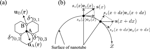
Figure 5: (a) The hexagonal lattice deformed by a phonon displacement vector. Let ${\bf u}_{\rm A}({\bf r})$ (${\bf u}_{\rm B}({\bf r})$) is a displacement vector of an A (B) site, then the modulation given by optical phonon modes is $\delta\gamma_{0,a}=(g/\ell){\bf u}({\bf r})\cdot{\bf R}_{a}$ where ${\bf u}({\bf r})$ ($={\bf u}_{\rm A}({\bf r})-{\bf u}_{\rm B}({\bf r})$) is a relative displacement vector of a B site relative to the nearest A site. (b) The cross section of a nanotube. The displacement vector for the RBM, ${\bf s}(x)$, is decomposed in terms of the normal $s_{z}(x)$ and tangential $s_{x}(x)$ components. The derivative of the normal unit vector ${\bf e}_{z}(x)$ with respect to $x$ gives a component along ${\bf e}_{x}(x)$, which modifies the net displacement along the $x$ direction.

The gauge field description for the el-ph interaction of the LO and TO modes (Eq. (22)) is useful to show the absence of the el-ph interaction for the TO mode with a finite wavevector, as shown below. The TO phonon mode with ${\bf q}\neq 0$ does not change the area of the hexagonal lattice but instead gives rise to a shear deformation. Thus, the TO mode (${\bf u}_{\rm TO}({\bf r})$) satisfies

$$\nabla\cdot{\bf u}_{\rm TO}({\bf r})=0,\ \ \ \ \nabla\times{\bf u}_{\rm TO}({\bf r})\neq 0.$$ (24)

Using Eqs. (22) and (24), we see that the TO mode does not yield a deformation-induced magnetic field,

$${\bf B}^{\rm q}({\bf r})\equiv\nabla\times{\bf A}^{\rm q}({\bf r}),$$ (25)

but the divergence of ${\bf A}^{\rm q}({\bf r})$ instead does not vanish because

$$\begin{split}&B^{\rm q}_{z}({\bf r})=-\frac{g}{v_{\rm F}}\nabla\cdot{\bf u}_{\rm TO}({\bf r})=0,\\ &\nabla\cdot{\bf A}^{\rm q}({\bf r})=\frac{g}{v_{\rm F}}(\nabla\times{\bf u}_{\rm TO}({\bf r}))\cdot{\bf e}_{z}\neq 0.\end{split}$$ (26)

Thus, we can define a scalar function $\varphi({\bf r})$ which satisfies ${\bf A}^{\rm q}({\bf r})=\nabla\varphi({\bf r})$. Since we can set ${\bf A}^{\rm q}({\bf r})=0$ in Eq. (18) by selecting the gauge as $\psi^{\rm K}({\bf r})\to\exp(-i\varphi({\bf r})/\hbar)\psi^{\rm K}({\bf r})$ [Sasaki et al. (2005)] and thus the ${\bf A}^{\rm q}({\bf r})$ in Eq. (18) disappears for the TO mode with ${\bf q}\neq 0$. This explains why the TO mode with ${\bf q}\neq 0$ is completely decoupled from the electrons, and that only the TO mode with ${\bf q}=0$ couples with electrons. This conclusion is valid even when the graphene sheet has a static surface deformation. In this sense, the TO phonon mode at the $\Gamma$-point is anomalous since the el-ph interaction for the TO mode can not be eliminated by a phase of the wavefunction. In contrast, the LO phonon mode with ${\bf q}\neq 0$ changes the area of the hexagonal lattice while it does not give rise to a shear deformation. Thus, the LO mode (${\bf u}_{\rm LO}({\bf r})$) satisfies

$$\nabla\cdot{\bf u}_{\rm LO}({\bf r})\neq 0,\ \ \ \ \nabla\times{\bf u}_{\rm LO}({\bf r})=0.$$ (27)

Using Eqs. (22) and (27), we see that the LO mode gives rise to a deformation-induced magnetic field since

$$B_{z}({\bf r})\neq 0,\ \ \ \nabla\cdot{\bf A}({\bf r})=0.$$ (28)

Since a magnetic field changes the energy band structure of electrons, the LO mode can couple strongly to the electrons even for ${\bf q}\neq 0$.

4.4 Deformation-Induced Gauge Field for the RBM

Next, we derive the deformation-induced gauge field ${\bf A}^{\rm q}({\bf r})$ for the RBM. When the RBM displacement vector of a carbon atom at ${\bf r}$ is ${\bf s}({\bf r})=(s_{x}({\bf r}),s_{y}({\bf r}),s_{z}({\bf r}))$, the perturbation to the nearest-neighbor hopping integral is given by

$$\delta\gamma_{0,a}({\bf r})=\frac{g}{\ell}{\bf R}_{a}\cdot\{{\bf s}({\bf r}+{\bf R}_{a})-{\bf s}({\bf r})\},$$ (29)

By expanding ${\bf s}({\bf r}+{\bf R}_{a})$ in a Taylor’s series around the displacement ${\bf s}({\bf r})$ as ${\bf s}({\bf r}+{\bf R}_{a})={\bf s}({\bf r})+({\bf R}_{a}\cdot\nabla){\bf s}({\bf r})+\cdots$, we approximate Eq. (29) as

$$\delta\gamma_{0,a}({\bf r})\simeq\frac{g}{\ell}{\bf R}_{a}\cdot\left\{({\bf R}_{a}\cdot\nabla){\bf s}({\bf r})\right\}.$$ (30)

Putting ${\bf R}_{1}=a_{\rm cc}{\bf e}_{y}$, ${\bf R}_{2}=-(\sqrt{3}/2)a_{\rm cc}{\bf e}_{x}-(1/2)a_{\rm cc}{\bf e}_{y}$, and ${\bf R}_{3}=(\sqrt{3}/2)a_{\rm cc}{\bf e}_{x}-(1/2)a_{\rm cc}{\bf e}_{y}$, into the right-hand side of Eq. (30), we obtain the corresponding deformation-induced gauge field of Eq. (19) as

$$\begin{split}&v_{\rm F}A^{\rm q}_{x}({\bf r})=\frac{ga_{\rm cc}}{2}\left[-\frac{\partial s_{x}({\bf r})}{\partial x}+\frac{\partial s_{y}({\bf r})}{\partial y}\right],\\ &v_{\rm F}A^{\rm q}_{y}({\bf r})=\frac{ga_{\rm cc}}{2}\left[\frac{\partial s_{x}({\bf r})}{\partial y}+\frac{\partial s_{y}({\bf r})}{\partial x}\right].\end{split}$$ (31)

Further, the displacements of carbon atoms give an on-site deformation potential in which the diagonal Hamiltonian matrix elements are modified by the el-ph interaction [Jiang et al. (2005); Saito and Kamimura (1983)]

$${\cal H}_{\rm on}=g_{\rm on}\sigma_{0}\left[\frac{\partial s_{x}({\bf r})}{\partial x}+\frac{\partial s_{y}({\bf r})}{\partial y}\right].$$ (32)

Here, $\partial s_{x}({\bf r})/\partial x+\partial s_{y}({\bf r})/\partial y$ ($=\nabla\cdot{\bf S}({\bf r})$) represents the change of the area of a graphene sheet [Suzuura and Ando (2002)]. According to the density functional calculation by Porezag et al. (1995), we adopt the on-site coupling constant $g_{\rm on}=17$[eV].

Since Eqs. (31) and (32) are proportional to the derivatives of $s_{x}({\bf r})$ and $s_{y}({\bf r})$, that is, they are proportional to ${\bf q}$, where ${\bf q}$ is the phonon wave vector. Then, the el-ph matrix element for the in-plane longitudinal/transverse acoustic (LA/TA) phonon modes vanishes at the $\Gamma$ point Namely, ${\bf A}^{\rm q}({\bf r})=0$ and ${\cal H}_{\rm on}=0$ in the limit of ${\bf q}=0$. Among the TA phonon modes, there is an out-of-plane TA (oTA) phonon mode. The oTA mode thus shifts carbon atoms on the flat 2D graphene sheet in the $z$-direction [see Fig. 4 and Fig. 5(b)]. The oTA mode of graphene corresponds to the RBM of a nanotube even though the RBM is not an acoustic phonon mode [Saito et al. (1998)]. In the following, we will show that the el-ph interaction for the RBM is enhanced due to the curvature of the nanotube as compared with the oTA mode of graphene since the RBM is a bond-stretching mode due to the cylindrical structure of SWNTs.

The displacements of the RBM modify the radius of a nanotube as $r\to r+s_{z}({\bf r})$ (see Fig. 5(b)). A change of the radius gives rise to two effects to the electronic state. One effect is a shift of the quantized transverse wave vector around the tube axis. The distance between two wave vectors around the tube axis depends on the inverse of the radius due to the periodic boundary condition, and a change of the radius results in a shift of the wavevector. The other effect is that the RBM can change the area on the surface of the nanotube even at the $\Gamma$ point. This results in an enhancement of the on-site el-ph interaction. These two effects are relevant to the fact that the normal vector on the surface of a nanotube is pointing in a different direction depending on the atom position. To show this, we take a (zigzag) nanotube as shown in Fig. 5(b). Let us denote the displacement vectors of two carbon atoms at $x$ and $x+dx$ as ${\bf s}(x)$ and ${\bf s}(x+dx)$, then an effective length for the displacement along the $x$ axis between the nearest two atoms is given by

$$D_{x}={\bf e}_{x}(x+dx)\cdot\left[{\bf s}(x+dx)-{\bf s}(x)\right].$$ (33)

By decomposing ${\bf s}(x)$ in terms of a normal and a tangential unit vector as ${\bf s}(x)=s_{z}(x){\bf e}_{z}(x)+s_{x}(x){\bf e}_{x}(x)$ (see Fig. 4(b)), we see that Eq. (33) becomes

$$D_{x} =s_{x}(x+dx)+s_{z}(x+dx){\bf e}_{x}(x+dx)\cdot{\bf e}_{z}(x+dx)$$

$$-s_{x}(x){\bf e}_{x}(x+dx)\cdot{\bf e}_{x}(x)-s_{z}(x){\bf e}_{x}(x+dx)\cdot{\bf e}_{z}(x)$$

$$=dx\left\{\frac{\partial s_{x}(x)}{\partial x}+\frac{s_{z}(x)}{r}\right\}+\cdots,$$ (34)

where we have used the following equations:

$$\begin{split}&{\bf e}_{z}(x+dx)={\bf e}_{z}(x)+\frac{dx}{r}{\bf e}_{x}(x)+\cdots,\\ &{\bf e}_{x}(x+dx)={\bf e}_{x}(x)+\frac{dx}{r}{\bf e}_{z}(x)+\cdots.\end{split}$$ (35)

Equation (34) shows that the net displacement along the $x$ axis is modified by the curvature of the nanotube as $\partial_{x}s_{x}({\bf r})\to\partial_{x}s_{x}({\bf r})+s_{z}({\bf r})/r$. The correction is negligible for a graphene sheet ($r\to\infty$), but appears as an enhancement factor to the el-ph interaction in SWNTs.

The el-ph interaction for the RBM is included by replacing $\partial_{x}s_{x}({\bf r})$ with $\partial_{x}s_{x}({\bf r})+s_{z}({\bf r})/r$ in Eqs. (31) and (32). In Eq. (31), we have an additional deformation-induced gauge field,

$$v_{\rm F}A^{\rm q}_{x}({\bf r})=-\frac{ga_{\rm cc}}{2}\frac{s_{z}({\bf r})}{r},$$ (36)

for the RBM mode which gives rise to a shift of the wavevector around the tube axis even at ${\bf q}=0$. In Eq. (32), it is shown that the RBM produces an additional on-site deformation potential of $g_{\rm on}\sigma_{0}(s_{z}({\bf r})/r)$. Finally, we obtain the el-ph interaction for the $\Gamma$ point (${\bf q}=0$: ${\bf s}({\bf r})$ is a constant) RBM, as

$${\cal H}_{\rm RBM}=-\frac{ga_{\rm cc}}{2}\frac{s_{z}}{r}\sigma_{x}+g_{\rm on}\frac{s_{z}}{r}\sigma_{0}=\frac{2s_{z}}{d_{t}}\begin{pmatrix}g_{\rm on}&-\frac{ga_{\rm cc}}{2}\cr-\frac{ga_{\rm cc}}{2}&g_{\rm on}\end{pmatrix}.$$ (37)

This representation is for zigzag SWNTs. For a general $(n,m)$ SWNT with a chiral angle $\theta$, the el-ph interaction for the RBM becomes

$${\cal H}_{\rm RBM}(\theta)=\frac{2s_{z}}{d_{t}}\begin{pmatrix}g_{\rm on}&-\frac{ga_{\rm cc}}{2}e^{+i3\theta}\cr-\frac{ga_{\rm cc}}{2}e^{-i3\theta}&g_{\rm on}\end{pmatrix}.$$ (38)

See Sasaki et al. (2008a) for more details.

5 Kohn Anomaly Effect

Here we consider the el-ph matrix element as a function of the electron wavevector ${\bf k}$ for the LO and TO phonon modes and the RBM with ${\bf q}={\bf 0}$ (i.e., $\Gamma$-point). The displacement vector with ${\bf q}={\bf 0}$ is expressed by a position independent ${\bf u}=(u_{x},u_{y})$, by which an electron-hole pair is excited. The el-ph interaction with ${\bf q}={\bf 0}$ is relevant to phonon-softening phenomena for all three kinds of modes.

5.1 Matrix Element for Electron-hole Pair Creation

Let us first consider the case of a zigzag SWNT. In Fig. 4, we denote $y$ ($x$) as a coordinate along (around) the axis of a zigzag SWNT, and $u_{y}$ ($u_{x}$) are assigned to the LO (TO) phonon mode.  Thus, from Eq. (22), we have

$$\begin{split}&v_{\rm F}{\bf A}^{\rm q}_{\rm LO}=g(u_{y},0),\\ &v_{\rm F}{\bf A}^{\rm q}_{\rm TO}=g(0,-u_{x}).\end{split}$$ (39)

The direction of the gauge field ${\bf A}^{\rm q}({\bf r})$ is perpendicular to the phonon eigenvector ${\bf u}$ and the LO mode shifts the wavevector around the tube axis, which explains how the LO mode may induce a dynamical energy band-gap in metallic nanotubes [Dubay et al. (2002)]. Putting Eq. (39) into Eq. (23), we get

$$\begin{split}&{\cal H}^{\rm zig}_{\rm LO}=v_{\rm F}{\bf A}^{\rm q}_{\rm LO}\cdot\mbox{\boldmath$\sigma$}=gu_{y}\sigma_{x},\\ &{\cal H}^{\rm zig}_{\rm TO}=v_{\rm F}{\bf A}^{\rm q}_{\rm TO}\cdot\mbox{\boldmath$\sigma$}=-gu_{x}\sigma_{y}.\end{split}$$ (40)

The el-ph matrix element $V_{\bf k}$ for the electron-hole pair generation is given from Eqs. (14), (15) and (40), by $(\lambda={\rm LO},{\rm TO})$

$$\langle{\rm eh}({\bf k})|{\cal H}^{\rm zig}_{\rm\lambda}|\omega_{\lambda}\rangle\equiv\int(\psi^{\rm K}_{c,{\bf k}}({\bf r}))^{\dagger}{\cal H}^{\rm zig}_{\lambda}\psi^{\rm K}_{v,{\bf k}}({\bf r})d^{2}{\bf r}.$$ (41)

By calculating Eq. (41) for the LO mode with $(u_{x},u_{y})=(0,u)$ and for the TO mode with $(u_{x},u_{y})=(u,0)$, we get

$$\begin{split}&\langle{\rm eh}({\bf k})|{\cal H}^{\rm zig}_{\rm LO}|\omega_{\rm LO}\rangle=-igu\sin\Theta({\bf k}),\\ &\langle{\rm eh}({\bf k})|{\cal H}^{\rm zig}_{\rm TO}|\omega_{\rm TO}\rangle=-igu\cos\Theta({\bf k}),\end{split}$$ (42)

where $\Theta({\bf k})$ is defined by an angle of ${\bf k}=(k_{x},k_{y})$ measured from the $k_{x}$ axis.

Next, we consider the case of an armchair SWNT. In Fig. 4, $x$ ($y$) is the coordinate along (around) the axis and $u_{x}$ ($u_{y}$) is assigned to the LO (TO) phonon mode. Then, for an armchair SWNT, we get

$$\begin{split}&\langle{\rm eh}({\bf k})|{\cal H}^{\rm arm}_{\rm LO}|\omega_{\rm LO}\rangle=-igu\sin\theta({\bf k}),\\ &\langle{\rm eh}({\bf k})|{\cal H}^{\rm arm}_{\rm TO}|\omega_{\rm TO}\rangle=-igu\cos\theta({\bf k}).\end{split}$$ (43)

Note that $\theta({\bf k})$ for the armchair nanotube is given by rotating $\Theta({\bf k})$ for the zigzag nanotube by $\pi/2$ ($\theta({\bf k})=\Theta({\bf k})+\pi/2$). It is useful to define the $k_{1}$ ($k_{2}$) axis pointing in the direction of a general SWNT circumferential (axis) direction (see Fig. 6), and $\theta({\bf k})$ as the angle for the polar coordinate. Then,

$$\begin{split}&\langle{\rm eh}({\bf k})|{\cal H}_{\rm LO}|\omega_{\rm LO}\rangle=-igu\sin\theta({\bf k}),\\ &\langle{\rm eh}({\bf k})|{\cal H}_{\rm TO}|\omega_{\rm TO}\rangle=-igu\cos\theta({\bf k}).\end{split}$$ (44)

is valid regardless of the tube chirality if the phonon eigenvector of the LO (TO) phonon mode is in the direction along (around) the tube axis. This is because ${\hat{\bf p}}$ and ${\bf u}({\bf r})$ [and ${\bf A}^{\rm q}({\bf r})$] are transformed in the same way when we change the chiral angle [Sasaki et al. (2008a)]. As a result, there would be no chiral angle dependence for the el-ph matrix elements in Eq. (44). Note also that Eq. (44) shows that $\langle{\rm eh}({\bf k})|{\cal H}_{\lambda}|\omega_{\lambda}\rangle$ depends only on $\theta({\bf k})$ but not on $|{\bf k}|$, which means that the dependence of this matrix element on $E^{\rm eh}$ ($=2\hbar v_{\rm F}|{\bf k}|$) is negligible [see Fig. 6(b)].

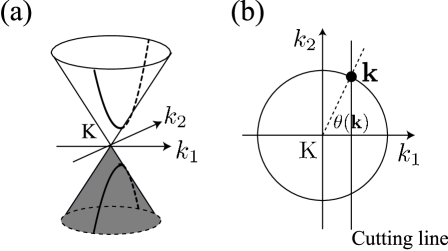
Figure 6: Dependence of LO and TO phonons on the cutting line. (a) A cutting line near the K-point. The $k_{1}$ ($k_{2}$) axis is selected as the nanotube circumferential (axis) direction. The amplitude for an electron-hole pair creation depends strongly on the relative position of the cutting line from the K-point. (b) If the cutting line crosses the K-point, then the angle $\theta({\bf k})$ ($\equiv\arctan(k_{2}/k_{1})$) takes $\pi/2$ ($-\pi/2$) values for $k_{2}>0$ ($k_{2}<0$). In this case, the LO mode strongly couples to an electron-hole pair, while the TO mode is decoupled from the electron-hole pair according to Eq. (43).

Where does the $\theta({\bf k})$ dependence in Eq. (44) then come form? The expectation value of $\sigma_{x}$, $\sigma_{y}$, and $\sigma_{z}$ with respect to $\psi^{\rm K}_{{\rm c},{\bf k}}({\bf r})$ defines the pseudospin. Using Eq. (14) with $\Theta({\bf k})\to\theta({\bf k})$, we have the expectation values for the Pauli matrices $\langle\sigma_{x}\rangle=\langle\psi^{\rm K}_{{\rm c},{\bf k}}|\sigma_{x}|\psi^{\rm K}_{{\rm c},{\bf k}}\rangle=\cos\theta({\bf k})$, $\langle\sigma_{x}\rangle=\langle\psi^{\rm K}_{{\rm c},{\bf k}}|\sigma_{y}|\psi^{\rm K}_{{\rm c},{\bf k}}\rangle=\sin\theta({\bf k})$, and $\langle\sigma_{x}\rangle=\langle\psi^{\rm K}_{{\rm c},{\bf k}}|\sigma_{z}|\psi^{\rm K}_{{\rm c},{\bf k}}\rangle=0$. Then the direction of the pseudospin of $\psi^{\rm K}_{{\rm c},{\bf k}}({\bf r})$,

$$(\langle\sigma_{x}\rangle,\langle\sigma_{y}\rangle,\langle\sigma_{z}\rangle)=(\cos\theta({\bf k}),\sin\theta({\bf k}),0),$$ (45)

is within $(k_{1},k_{2})$ plane and parallel to ${\bf k}$ (see Fig. 7).  Due to the particle-hole symmetry, $\psi^{\rm K}_{v,{\bf k}}({\bf r})=\sigma_{z}\psi^{\rm K}_{c,{\bf k}}({\bf r})$, the el-ph matrix element for the electron-hole pair creation process can be related to the pseudospin. For example, we see that

$$\langle{\rm eh}({\bf k})|{\cal H}^{\rm zig}_{\rm LO}|\omega_{\rm LO}\rangle =gu_{y}\langle\psi^{\rm K}_{{\rm c},{\bf k}}|\sigma_{x}|\psi^{\rm K}_{{\rm v},{\bf k}}\rangle$$

$$=gu\langle\psi^{\rm K}_{{\rm c},{\bf k}}|\sigma_{x}\sigma_{z}|\psi^{\rm K}_{{\rm c},{\bf k}}\rangle$$

$$=-igu\langle\sigma_{y}\rangle$$

$$=-igu\sin\theta({\bf k}).$$ (46)

The electron-hole pair creation for the LO mode is relevant to the pseudospin component which is parallel to the tube axis, $\langle\sigma_{y}\rangle$, while that for the TO mode is relevant to $\langle\sigma_{x}\rangle$.

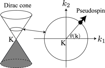
Figure 7: The el-ph matrix element for the electron-hole pair creation process relates to the pseudospin of the electronic state.

For RBM, from Eq. (38), the matrix element for an electron-hole pair creation is chirality dependent as

$$\langle{\rm eh}({\bf k})|{\cal H}_{\rm RBM}(\theta)|\omega_{\rm RBM}\rangle=iga_{\rm cc}\frac{s_{z}}{d_{t}}\sin(\theta({\bf k})+3\theta).$$ (47)

Thus, the frequency shift of the RBM can have a chiral angle dependence. In particular, armchair SWNTs ($\theta=30^{\circ}$) exhibit neither a frequency shift nor a broadening, regardless of their diameters because the el-ph matrix element becomes

$$\langle{\rm eh}({\bf k})|{\cal H}^{\rm arm}_{\rm RBM}|\omega_{\rm RBM}\rangle=iga_{\rm cc}\frac{s_{z}}{d_{t}}\cos\theta({\bf k}),$$ (48)

which is zero for a cutting line for a metallic band: $\theta({\bf k})=\pm\pi/2$. This $\theta({\bf k})$ dependence of Eq. (48) is the same as that of the TO phonon mode of Eq. (43), so that the absence of a frequency shift of the RBM in armchair SWNTs is similar to the absence of a frequency shift of the TO mode at the $\Gamma$ point in armchair SWNTs [Sasaki et al. (2008b)].

5.2 Phonon frequency shift

Here we show the calculated results for the phonon frequency as a function of the Fermi energy.

5.2.1 Armchair SWNTs

First, we consider Eq. (44) for a $k$-point (${\bf k}=(k_{1},k_{2})$) on the cutting line of an armchair SWNT. Since the armchair SWNT is free from the curvature effect, the cutting line for its metallic energy band satisfies $k_{1}=0$ and lies on the $k_{2}$ axis. Thus, we have $\theta({\bf k})=\pi/2$ ($-\pi/2$) for $k_{2}>0$ ($k_{2}<0$). Then, Eq. (44) tells us that only the LO mode can couple to an electron-hole pair and the TO mode does not couple to an electron-hole pair for the metallic energy band of an armchair SWNT. Similarly, Eq. (48) shows that the RBM of an armchair SWNT does not show any phonon softening.

In Fig. 8, we show the phonon energy as a function of $E_{\rm F}$ for a $(10,10)$ armchair SWNT. Here we take 1620 ${\rm cm}^{-1}$ and 1590 ${\rm cm}^{-1}$ for $\hbar\omega$ of the LO and TO modes, respectively. The energy bars denote $\Gamma$ values. The self-energy is calculated for $T=300$K and $L=10{\rm\mu m}$. It is shown that the TO mode does not exhibit any energy change, while the LO mode shows both an energy shift and a broadening. As we have mentioned, the minimum energy is realized at $|E_{\rm F}|=\hbar\omega/2$ ($\approx 0.1$ eV). There is a local maximum for the spectral peak at $|E_{\rm F}|=0$. The broadening for the LO mode has a tail at room temperature for $|E_{\rm F}|>\hbar\omega/2$.

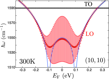
Figure 8: (color online) The $E_{\rm F}$ dependence of the LO (red curve) and TO (black curve) phonon energy in the case of the $(10,10)$ armchair SWNT. The data are taken at room temperature. Only the energy of the LO mode is shifted, with the TO mode frequency being independent of $E_{\rm F}$. The decay width ($\Gamma$) is plotted as an error-bar. The blue curve is given by the analytic result of Eq. (49).

In evaluating the LO mode’s self-energy according to Eq. (7), we have assumed that the cutoff energy is $E_{c}=0.5$eV. The presence of a cutoff energy is reasonable since the matrix element actually depends on the energy of the electron-hole pair [see Sasaki et al. (2009)]. An analytical expression for the $E_{c}$ dependence of the self-energy is easy to obtain by using the effective-mass model, which can be derived from Eq. (7) at $T=0$ as

$${\rm Re}\left[\Pi(\omega,E_{\rm F})\right]\approx-\frac{L}{\pi}\left(\frac{A^{\rm q}_{\rm LO}}{\hbar}\right)^{2}\hbar v_{\rm F}\left[\ln\left|\frac{E_{c}-\frac{\hbar\omega}{2}}{|E_{\rm F}|-\frac{\hbar\omega}{2}}\right|+\ln\left|\frac{E_{c}+\frac{\hbar\omega}{2}}{|E_{\rm F}|+\frac{\hbar\omega}{2}}\right|\right].$$ (49)

The factor scales as $1/d_{t}$ because 

$$\frac{L}{\pi}\left(\frac{A^{\rm q}_{\rm LO}}{\hbar}\right)^{2}\hbar v_{\rm F}\approx 4[{\rm meV}]\left(\frac{[{\rm nm}]}{d_{t}}\right).$$ (50)

For comparison, we plot $\hbar\omega+{\rm Re}\left[\Pi(\omega,E_{\rm F})\right]$ (Eq. (49)) as the blue curve in Fig. 8.

5.2.2 Zigzag SWNTs

Next we consider “metallic” zigzag SWNTs. When the curvature effect is taken into account, the cutting line does not lie on the K-point, but is shifted by $k_{1}$ from the $k_{2}$ axis. In this case, $\cos\theta({\bf k})=k_{1}/(k_{1}^{2}+k_{2}^{2})^{1/2}$ is nonzero for the lower energy intermediate electron-hole pair states. Thus, the TO mode can couple to the low energy electron-hole pair which makes a positive energy contribution to the phonon energy shift. The high energy electron-hole pair still decouples from the TO mode since $\cos\theta({\bf k})\to 0$ for $|k_{2}|\gg|k_{1}|$.

In Fig. 9(a), we show calculated results for the LO and TO modes as a function of $E_{\rm F}$ for a $(12,0)$ zigzag SWNT. In the case of zigzag SWNTs, not only the LO mode but also the TO mode couples with electron-hole pairs. The spectrum peak position for the TO mode becomes harder (upshifted) for $E_{\rm F}=0$, since ${\rm Re}(h_{+}(E^{\rm eh}))$ for $E^{\rm eh}<\hbar\omega$ contributes to a positive frequency shift. The hardening of the TO mode is a signature of the curvature-induced mini-energy gap.

In Fig. 9(b), we show the result for the RBM. The matrix element of Eq. (47) with $\theta=0^{\circ}$ is proportional to $\sin\theta({\bf k})$. Thus, the high energy electron-hole pair can couple to the RBM and can contribute to the softening of the RBM. Although the magnitude of the shift is smaller than those for the LO mode, the softening for the RBM can be observed experimentally [Farhat et al. (2009)].

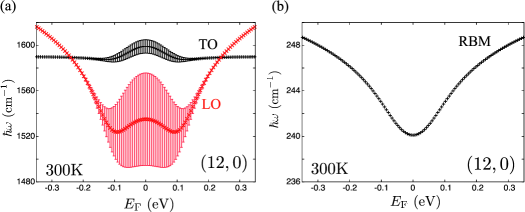
Figure 9: (color online) (a) The $E_{\rm F}$ dependence of the LO (red curve) and TO (black curve) phonon energy in the case of the $(12,0)$ zigzag SWNT. The data are taken at room temperature. Not only the frequency of the LO mode but also that of the TO mode is shifted due to the curvature effect. Here we take 1640 ${\rm cm}^{-1}$ and 1590 ${\rm cm}^{-1}$ for $\hbar\omega$ of the LO and TO modes, respectively. (b) The $E_{\rm F}$ dependence of the RBM energy $\hbar\omega$ in the case of the $(12,0)$ zigzag SWNT.

5.2.3 Chiral SWNTs

Finally, we examine “metallic” chiral SWNTs. The same discussion for the “metallic” zigzag SWNTs can be applied to “metallic” chiral SWNTs. However, there is a complication specific to chiral SWNTs that the phonon eigenvector depends on the chiral angle. Reich et al. (2001) reported that, for a chiral nanotube, the atoms vibrate along the direction of the carbon-carbon bonds and not along the axis or the circumference. The phonon eigenvector of a chiral nanotube may be written as

$$\begin{pmatrix}u_{\rm TO}\cr u_{\rm LO}\end{pmatrix}=\begin{pmatrix}\cos\phi&\sin\phi\cr-\sin\phi&\cos\phi\end{pmatrix}\begin{pmatrix}u_{1}\cr u_{2}\end{pmatrix},$$ (51)

where $u_{1}$ ($u_{2}$) is in the direction around (along) a chiral tube axis, and $\phi$ is the angle difference between the axis and the vibration. This modifies Eq. (43) as

$$\begin{split}&\langle{\rm eh}({\bf k})|{\cal H}_{\rm LO}|\omega_{\rm LO}\rangle=-igu\sin(\theta({\bf k})+\phi),\\ &\langle{\rm eh}({\bf k})|{\cal H}_{\rm TO}|\omega_{\rm TO}\rangle=-igu\cos(\theta({\bf k})+\phi).\end{split}$$ (52)

The identification of $\phi$ in Eq. (52) as a function of chirality would be useful to compare theoretical results and experiments, which will be explored in the future [See Park et al. (2009) for example].

5.2.4 Graphene

In the case of 2D graphene, Eq. (43) tells us that the $\Gamma$ point TO and LO modes give the same energy shift because the integral over $\theta({\bf k})$ gives the same self-energy in Eq. (7) for both TO and LO modes. This explains why no $G$-band splitting is observed in a single layer of graphene [Yan et al. (2007)]. Even when we consider the TO and LO modes not exactly at the $\Gamma$ point, we do not expect any splitting between the LO and TO phonon energies since the TO mode with ${\bf q}\neq 0$ is completely decoupled from the electrons [see Eq. (26)]. Thus, for ${\bf q}\neq 0$, only the LO mode contributes to the $G$ band intensity. It is interesting to note that the $\Gamma$ point LO and TO modes may exhibit anomalous behavior near the edge of graphene because the wave function is not given by a plane wave but rather by a standing wave. The pseudospin for the standing wave is different from that for a plane wave. Moreover, the standing wave near the zigzag edge is different from that near the armchair edge, which gives rise to a selection rule in their Raman spectra [Sasaki et al. (2009, 2010)]. The standing wave behavior near the edges in graphene ribbons is beyond the scope of the present paper.

6 Discussion and Summary

We have seen that the curvature-induced gap is absent for armchair SWNTs, so that here the LO mode exhibits a strong Kohn anomaly effect. Recently, however, it has been reported that even armchair SWNTs have an energy gap originating from a correlation effect [Deshpande et al. (2009)]. The correlation-induced gap observed is approximately 80 meV for armchair SWNT with $d_{t}=2$nm, and the gap increases with decreasing $d_{t}$. Since the presence of a gap suppresses the contribution to the hardening, a local maximum (around $E_{\rm F}=0$) in the LO frequency vs. $E_{\rm F}$ plot [see Fig. 8] may disappear, and $E_{\rm F}=0$ would become a global minimum if the correlation gap exceeds 200meV. Confirming this behavior in a Raman spectroscopy study may provide further evidence for the correlation-induced gap.

Finally, we discuss our results in relation to the experimental results of the Kohn anomaly for the RBMs in metallic SWNTs [Farhat et al. (2009)]. The frequency shifts observed are approximately 2cm^-1, which is smaller than the theoretical value for a $(12,0)$ zigzag SWNT, 8cm^-1, shown in Fig. 9(b). This discrepancy may be attributed to the choice of the off-site el-ph matrix element, $g$, although we have determined this value from density functional calculation. Indeed, by decreasing the value of $g$ from $g=6.4$ eV/Å we find a better agreement to the experimental result, 3cm^-1 when $g=4$ eV/Å. Another possibility is that we have used a harmonic oscillator model for obtaining the magnitude of displacement vector $u$. Actual value of $u$ may be smaller than our estimation, which also gives a better agreement to the experimental result.

In summary, the el-ph interaction with respect to the LO, TO, and RBM for the Raman feature for SWNTs is derived in a unified way using the deformation-induced gauge field. Then, we have shown that the matrix element for electron-hole pair creation depends on the position of the cutting line. As a result, the TO mode in “metallic” SWNTs, except for armchair SWNTs, can couple to an electron-hole pair due to the curvature effect which shifts the cutting line away from the K point. In particular, only the low energy electron-hole pairs can couple to the TO mode and give rise to a hardening of the TO mode. The hardening of the TO mode is suppressed for large diameter SWNTs. This is reasonable since the TO mode as well as the LO mode exhibit a softening in the case of graphene samples.

References

- Ando (2000) Ando, T., 2000. Spin-orbit interaction in carbon nanotubes. J. Phys. Soc. Jpn. 69, 1757–1763.
- Ando (2008) Ando, T., 2008. Optical phonon tuned by fermi level in carbon nanotubes. J. Phys. Soc. Jpn. 77, 014707.
- Bachilo et al. (2002) Bachilo, S., Strano, M., Kittrell, C., Hauge, R., Smalley, R., Weisman, R., 2002. Structure-assigned optical spectra of single-walled carbon nanotubes. Science 298, 2361.
- Caudal et al. (2007) Caudal, N., Saitta, A. M., Lazzeri, M., Mauri, F., 2007. Kohn anomalies and nonadiabaticity in doped carbon nanotubes. Phy. Rev. B 75 (11), 115423.
- Das et al. (2007) Das, A., Sood, A. K., Govindaraj, A., Saitta, A. M., Lazzeri, M., Mauri, F., Rao, C. N. R., 2007. Doping in carbon nanotubes probed by raman and transport measurements. Phys. Rev. Lett. 99 (13), 136803.
- Deshpande et al. (2009) Deshpande, V. V., Chandra, B., Caldwell, R., Novikov, D. S., Hone, J., Bockrath, M., 2009. Mott Insulating State in Ultraclean Carbon Nanotubes. Science 323 (5910), 106–110.
- Dresselhaus et al. (2005) Dresselhaus, M. S., Dresselhaus, G., Saito, R., Jorio, A., 2005. Raman spectroscopy of carbon nanotubes. Physics Reports 409, 47–99.
- Dubay and Kresse (2003) Dubay, O., Kresse, G., Jan 2003. Accurate density functional calculations for the phonon dispersion relations of graphite layer and carbon nanotubes. Phys. Rev. B 67 (3), 035401.
- Dubay et al. (2002) Dubay, O., Kresse, G., Kuzmany, H., 2002. Phonon softening in metallic nanotubes by a peierls-like mechanism. Phys. Rev. Lett. 88 (23), 235506.
- Eklund et al. (1977) Eklund, P. C., Dresselhaus, G., Dresselhaus, M. S., Fischer, J. E., 1977. Raman scattering from in-plane lattice modes in low-stage graphite-alkali-metal compounds. Phys. Rev. B 16 (8), 3330–3333.
- Farhat et al. (2009) Farhat, H., Sasaki, K., Kalbac, M., Hofmann, M., Saito, R., Dresselhaus, M. S., Kong, J., 2009. Softening of the radial breathing mode in metallic carbon nanotubes. Phys. Rev. Lett. 102 (12), 126804.
- Farhat et al. (2007) Farhat, H., Son, H., Samsonidze, G. G., Reich, S., Dresselhaus, M. S., Kong, J., 2007. Phonon softening in individual metallic carbon nanotubes due to the kohn anomaly. Phys. Rev. Lett. 99 (14), 145506.
- Hamada et al. (1992) Hamada, N., Sawada, S.-i., Oshiyama, A., 1992. New one-dimensional conductors: Graphitic microtubules. Phys. Rev. Lett. 68 (10), 1579–1581.
- Ishikawa and Ando (2006) Ishikawa, K., Ando, T., 2006. Optical phonon interacting with electrons in carbon nanotubes. J. Phys. Soc. Jpn. 75, 084713.
- Jiang et al. (2005) Jiang, J., Saito, R., Samsonidze, G. G., Chou, S. G., Jorio, A., Dresselhaus, G., Dresselhaus, M. S., 2005. Electron-phonon matrix elements in single-wall carbon nanotubes. Phys. Rev. B 72, 235408.
- Jorio et al. (2003) Jorio, A., Pimenta, M. A., Filho, A. G. S., Saito, R., Dresselhaus, G., Dresselhaus, M. S., 2003. Characterizing carbon nanotube samples with resonance raman scattering. New Journal of Physics 5, 139.
- Jorio et al. (2001) Jorio, A., Saito, R., Hafner, J. H., Lieber, C. M., Hunter, M., McClure, T., Dresselhaus, G., Dresselhaus, M. S., 2001. Structural determination of isolated single-wall carbon nanotubes by resonant Raman scattering. Phys. Rev. Lett. 86, 1118–1121.
- Jorio et al. (2002) Jorio, A., Souza Filho, A. G., Dresselhaus, G., Dresselhaus, M. S., Swan, A. K., Ünlü, M. S., Goldberg, B. B., Pimenta, M. A., Hafner, J. H., Lieber, C. M., Saito, R., 2002. -band resonant raman study of 62 isolated single-wall carbon nanotubes. Phys. Rev. B 65 (15), 155412.
- Kane and Mele (1997) Kane, C. L., Mele, E. J., 1997. Size, shape, and low energy electronic structure of carbon nanotubes. Phys. Rev. Lett. 78 (10), 1932–1935.
- Katsnelson and Geim (2008) Katsnelson, M., Geim, A., 2008. Electron scattering on microscopic corrugations in graphene. Phil. Trans. R. Soc. A 366, 195.
- Kleiner and Eggert (2001) Kleiner, A., Eggert, S., 2001. Band gaps of primary metallic carbon nanotubes. Phys. Rev. B 63 (7), 73408.
- Kohn (1959) Kohn, W., 1959. Image of the fermi surface in the vibration spectrum of a metal. Phys. Rev. Lett. 2 (9), 393–394.
- Lazzeri and Mauri (2006) Lazzeri, M., Mauri, F., 2006. Nonadiabatic kohn anomaly in a doped graphene monolayer. Phys. Rev. Lett. 97 (26), 266407.
- Mintmire et al. (1992) Mintmire, J. W., Dunlap, B. I., White, C. T., 1992. Are fullerene tubules metallic? Phys. Rev. Lett. 68 (5), 631–634.
- Miyake and Saito (2005) Miyake, T., Saito, S., 2005. Band-gap formation in single-walled carbon nanotubes : A first-principles study. Phys. Rev. B 72 (7), 73404.
- Nguyen et al. (2007) Nguyen, K. T., Gaur, A., Shim, M., 2007. Fano lineshape and phonon softening in single isolated metallic carbon nanotubes. Phys. Rev. Lett. 98 (14), 145504.
- Ouyang et al. (2001) Ouyang, M., Huang, J.-L., Cheung, C. L., Lieber, C. M., 2001. Energy gaps in ”metallic” single-walled carbon nanotubes. Science 292, 702.
- Park et al. (2009) Park, J. S., Sasaki, K., Saito, R., Izumida, W., Kalbac, M., Farhat, H., Dresselhaus, G., Dresselhaus, M. S., 2009. Fermi energy dependence of the g-band resonance raman spectra of single-wall carbon nanotubes. Phys. Rev. B 80, 81402.
- Pimenta et al. (1998) Pimenta, M. A., Marucci, A., Empedocles, S. A., Bawendi, M. G., Hanlon, E. B., Rao, A. M., Eklund, P. C., Smalley, R. E., Dresselhaus, G., Dresselhaus, M. S., 1998. Raman modes of metallic carbon nanotubes. Phys. Rev. B 58, R16016.
- Piscanec et al. (2004) Piscanec, S., Lazzeri, M., Mauri, F., Ferrari, A. C., Robertson, J., 2004. Kohn anomalies and electron-phonon interactions in graphite. Phys. Rev. Lett. 93, 185503.
- Popov (2004) Popov, V. N., 2004. Curvature effects on the structural, electronic and optical properties of isolated single-walled carbon nanotubes within a symmetry-adapted non-orthogonal tight-binding model. New Journal of Physics 6, 17.
- Popov and Lambin (2006) Popov, V. N., Lambin, P., 2006. Radius and chirality dependence of the radial breathing mode and the g-band phonon modes of single-walled carbon nanotubes. Phys. Rev. B 73 (8), 85407.
- Porezag et al. (1995) Porezag, D., Frauenheim, T., Köhler, T., Seifert, G., Kaschner, R., May 1995. Construction of tight-binding-like potentials on the basis of density-functional theory: Application to carbon. Phys. Rev. B 51 (19), 12947–12957.
- Reich et al. (2001) Reich, S., Thomsen, C., Ordejón, P., 2001. Phonon eigenvectors of chiral nanotubes. Phys. Rev. B 64 (19), 195416.
- Saito et al. (1998) Saito, R., Dresselhaus, G., Dresselhaus, M., 1998. Physical Properties of Carbon Nanotubes. Imperial College Press, London.
- Saito et al. (1992a) Saito, R., Fujita, M., Dresselhaus, G., Dresselhaus, M. S., 1992a. Electronic structure of chiral graphene tubules. Appl. Phys. Lett. 60, 2204–2206.
- Saito et al. (1992b) Saito, R., Fujita, M., Dresselhaus, G., Dresselhaus, M. S., 1992b. Electronic structures of carbon fibers based on C60. Phys. Rev. B 46, 1804–1811.
- Saito et al. (2003) Saito, R., Gruneis, A., Samsonidze, G. G., Brar, V. W., Dresselhaus, G., Dresselhaus, M. S., Jorio, A., Cancado, L. G., Fantini, C., Pimenta, M. A., Filho, A. G. S., 2003. Double resonance raman spectroscopy of single-wall carbon nanotubes. New Journal of Physics 5, 157.
- Saito and Kamimura (1983) Saito, R., Kamimura, H., 1983. Vibronic states of polyacetylene, (ch)x. J. Phys. Soc. Jpn. 52, 407.
- Samsonidze et al. (2004) Samsonidze, G. G., Saito, R., Kobayashi, N., Grüneis, A., Jiang, J., Jorio, A., Chou, S. G., Dresselhaus, G., Dresselhaus, M. S., 2004. Family behavior of the optical transition energies in single-wall carbon nanotubes of smaller diameters. Appl. Phys. Lett. 85, 5703.
- Sasaki et al. (2005) Sasaki, K., Kawazoe, Y., Saito, R., 2005. Local energy gap in deformed carbon nanotubes. Prog. Theor. Phys. 113 (3), 463–480.
- Sasaki et al. (2006) Sasaki, K., Murakami, S., Saito, R., 2006. Gauge field for edge state in graphene. J. Phys. Soc. Jpn. 75, 074713.
- Sasaki and Saito (2008) Sasaki, K., Saito, R., 2008. Pseudospin and deformation-induced gauge field in graphene. Prog. Theor. Phys. Suppl. 176, 253–278.
- Sasaki et al. (2008a) Sasaki, K., Saito, R., Dresselhaus, G., Dresselhaus, M. S., Farhat, H., Kong, J., 2008a. Chirality-dependent frequency shift of radial breathing mode in metallic carbon nanotubes. Phys. Rev. B 78 (23), 235405.
- Sasaki et al. (2008b) Sasaki, K., Saito, R., Dresselhaus, G., Dresselhaus, M. S., Farhat, H., Kong, J., 2008b. Curvature-induced optical phonon frequency shift in metallic carbon nanotubes. Phys. Rev. B 77 (24), 245441.
- Sasaki et al. (2010) Sasaki, K., Saito, R., Wakabayashi, K., Enoki, T., 2010. Identifying the orientation of edge of graphene using g band raman spectra. to appear in J. Phys. Soc. Jpn. [arXiv:0911.1593].
- Sasaki et al. (2009) Sasaki, K., Yamamoto, M., Murakami, S., Saito, R., Dresselhaus, M., Takai, K., Mori, T., Enoki, T., Wakabayashi, K., 2009. Kohn anomalies in graphene nanoribbons. Phys. Rev. B 80 (15), 155450.
- Strano et al. (2003) Strano, M., Doorn, S., Haroz, E., Kittrell, C., Hauge, R., Smalley, R., 2003. Assignment of (n, m) raman and optical features of metallic single-walled carbon nanotubes. Nano Letters 3 (8), 1091–1096.
- Suzuura and Ando (2002) Suzuura, H., Ando, T., May 2002. Phonons and electron-phonon scattering in carbon nanotubes. Phys. Rev. B 65 (23), 235412.
- Yan et al. (2007) Yan, J., Zhang, Y., Kim, P., Pinczuk, A., 2007. Electric field effect tuning of electron-phonon coupling in graphene. Phy. Rev. Lett. 98 (16), 166802.
- Yang et al. (1999) Yang, L., Anantram, M. P., Han, J., Lu, J. P., 1999. Band-gap change of carbon nanotubes: Effect of small uniaxial and torsional strain. Phys. Rev. B 60, 13874–13878.
- Yang and Han (2000) Yang, L., Han, J., 2000. Electronic structure of deformed carbon nanotubes. Phys. Rev. Lett. 85, 154–157.