The origin of the hidden supersymmetry

Abstract

The hidden supersymmetry and related tri-supersymmetric structure of the free particle system, the Dirac delta potential problem and the Aharonov-Bohm effect (planar, bound state, and tubule models) are explained by a special nonlocal unitary transformation, which for the usual $N=2$ supercharges has a nature of Foldy-Wouthuysen transformation. We show that in general case, the bosonized supersymmetry of nonlocal, parity even systems emerges in the same construction, and explain the origin of the unusual $N=2$ supersymmetry of electron in three-dimensional parity even magnetic field. The observation extends to include the hidden superconformal symmetry.

1 Introduction

Some quantum systems possess a hidden symmetry associated with nontrivial integrals of motion, which reflect their peculiar properties. A hidden supersymmetry [1] was revealed recently in a class of quantum mechanical systems with a local Hamiltonian. The list of such systems includes the Dirac delta potential problem [2], the Aharonov-Bohm effect (bound state [2] and planar [3] models), the finite-gap periodic quantum systems, and their infinite period limit in the form of reflectionless systems [4, 5]. All the listed systems possess a degeneration in the energy spectrum associated with a (twisted) parity symmetry. The hidden supersymmetry of the first two systems is characterized by the linear in the momentum supercharge operators; in the last two families, the hidden supersymmetry is related to the higher derivative nontrivial operator of the Lax pair of the associated nonlinear integrable system. A usual $N=2$ superextension of all these systems is accompanied by a rich tri-supersymmetric structure rooted in the hidden supersymmetry [6, 7, 8]. A natural question arises whether the hidden and usual supersymmetry are somehow related.

In this paper we show how the hidden supersymmetry and the associated tri-supersymmetric structure originate from the usual $N=2$ supersymmetry and the (twisted) parity symmetry. The observation is illustrated by the models of the Dirac delta potential problem and the Aharonov-Bohm (AB) effect. We also discuss the nature of the earlier revealed bosonized supersymmetry of nonlocal spinless quantum systems with parity even potentials [1], that appears in the same construction, and explain the origin of the unusual $N=2$ supersymmetry of electron in three-dimensional parity-even magnetic field [9, 10]. Finally, we indicate that the observation extends to include the hidden superconformal symmetry [3], [11].

2 One-dimensional case: special unitary transformation

Consider an $N=2$ supersymmetric one-dimensional quantum mechanical system [12, 10, 13]. It is described by the Hamiltonian

$$H=P^{2}+W^{2}+\sigma_{3}W^{\prime},$$ (2.1)

and supercharges

$$Q_{1}=\sigma_{1}P+\sigma_{2}W,\qquad Q_{2}=i\sigma_{3}Q_{1}=-\sigma_{2}P+\sigma_{1}W,$$ (2.2)

where $P=-i\frac{d}{dx}$, $W=W(x)$ is a superpotential, $W^{\prime}={dW}/{dx}$, $2m=1$ and $\hbar=1$. The $H$ and $Q_{a}$, $a=1,2$, generate the $N=2$ supersymmetry,

$$\{Q_{a},Q_{b}\}=2\delta_{ab}H\,,\qquad[Q_{a},H]=0\,,$$ (2.3)

for which the integral $\Gamma=\sigma_{3}$ plays a role of the grading operator, $[\Gamma,H]=\{\Gamma,Q_{a}\}=0$.

Assume that the superpotential is an odd function, $W(-x)=-W(x)$. Then the Hamiltonian is the even operator. The reflection (parity) $\mathcal{R}$, $\mathcal{R}x=-x\mathcal{R}$, $\mathcal{R}^{2}=1$, is the additional, nonlocal integral of motion, $[\mathcal{R},H]=0$. It anticommutes with the supercharges, $\{\mathcal{R},Q_{a}\}=0$. Let us realize a unitary transformation,

$$\mathcal{O}\rightarrow\tilde{\mathcal{O}}=U\mathcal{O}U^{-1}\,,\qquad U=\exp(i\pi S_{-}\Pi_{-})=S_{+}+\mathcal{R}S_{-}=\left(\begin{array}[]{cc}\Pi_{+}&\Pi_{-}\\ \Pi_{-}&\Pi_{+}\end{array}\right),$$ (2.4)

where $S_{\pm}=\frac{1}{2}(1\pm\sigma_{1})$ and $\Pi_{\pm}=\frac{1}{2}(1\pm\mathcal{R})$ are the projectors. The (nonlocal) operator (2.4) satisfies $U^{\dagger}=U^{-1}=U$, so that $U^{2}=1$. We have $\tilde{x}=x\sigma_{1}$, $\tilde{P}=P\sigma_{1}$, $\tilde{\mathcal{R}}=\mathcal{R}$, $\tilde{\sigma}_{1}=\sigma_{1}$, $\tilde{\sigma}_{2}=\sigma_{2}\mathcal{R}$, $\tilde{\sigma}_{3}=\sigma_{3}\mathcal{R}$, and the transformed Hamiltonian and supercharges take a diagonal form,

$$\tilde{H}=P^{2}+W^{2}+\sigma_{3}\mathcal{R}W^{\prime}\,,$$ (2.5)

$$\tilde{Q}_{1}=P-i\sigma_{3}\mathcal{R}W\,,\qquad\tilde{Q}_{2}=W+i\sigma_{3}\mathcal{R}P\,.$$ (2.6)

For the first order supercharge operators (2.2), this transformation has a nature of Foldy-Wouthuysen transformation. We trade the locality of the operators for their diagonal form. The transformed operators (2.5) and (2.6) satisfy the same $N=2$ superalgebra,

$$\{\tilde{Q}_{a},\tilde{Q}_{b}\}=2\delta_{ab}\tilde{H}\,,\qquad[\tilde{Q}_{a},\tilde{H}]=0\,,$$ (2.7)

for which

$$\tilde{\Gamma}=\sigma_{3}\mathcal{R}$$ (2.8)

plays a role of the grading operator.

Notice that the unitary transformation (2.4) mediates the intertwining relation $U\mathcal{O}=\tilde{\mathcal{O}}U$ between the corresponding Hamiltonians, supercharges and grading operators.

In general, the transformed Hamiltonian (2.5) differs from the original, local Hamiltonian (2.1). Though by the construction the both are unitary equivalent, the Hamiltonian (2.5) is nonlocal due to the presence of the reflection operator in the last term. There are particular cases, however, for which the nonlocality is suppressed by a specific choice of the superpotential, and $\tilde{H}=H$. We will discuss some of such systems later in the text.

The operators (2.2) are not integrals of motion for the transformed Hamiltonian (2.5), while the transformed supercharges (2.6) do not commute with the initial Hamiltonian (2.1). At the same time, the three operators $\sigma_{3}$, $\mathcal{R}$ and $\mathcal{R}\sigma_{3}$ are the integrals for both $H$ and $\tilde{H}$. The supercharges $Q_{a}$ commute with $\sigma_{3}\mathcal{R}$, while the transformed supercharges $\tilde{Q}_{a}$ commute with $\sigma_{3}$. Both the original and the transformed supercharges anticommute with $\mathcal{R}$. It is worth to note that there exists no unitary transformation that would transform $\sigma_{3}$ (or $\mathcal{R}\sigma_{3}$) into $\mathcal{R}$.

The transformed system (2.5) can be reduced to any of the two eigensubspaces of $\sigma_{3}$. Each of the obtained spinless nonlocal systems,

$$\tilde{H}_{s}=P^{2}+W^{2}+s\mathcal{R}W^{\prime}\,,\quad{\rm where}\quad s=+1\quad{\rm or}\quad s=-1\,,$$ (2.9)

still possesses a bosonized $N=2$ supersymmetry described by the nonlocal supercharges,

$$\tilde{Q}_{1,s}=P-is\mathcal{R}W\,,\qquad\tilde{Q}_{2,s}=W+is\mathcal{R}P=is\mathcal{R}\tilde{Q}_{1,s}\,.$$ (2.10)

The operator $\mathcal{R}$ plays the role of the grading operator for both ($s=\pm 1$) reduced systems. Such nonlocal supersymmetric systems were investigated in [1]. Here, we just illustrate a general situation by a simple example of the super-oscillator system given by $W(x)=x$, see Fig. 1. In this case the reduced Hamiltonians can be presented in the form $\tilde{H}_{+}=2(N+\Pi_{+})$ ($s=+1$) and $\tilde{H}_{-}=2(N+\Pi_{-})$ ($s=-1$), where $N=a^{+}a^{-}$ is a number operator, $\Pi_{\pm}=\frac{1}{2}(1\pm\mathcal{R})$ are the projectors on subspaces with even and odd eigenvalues of $N$, and the reflection operator, $\mathcal{R}=(-1)^{N}=\cos{\pi N}$, being written in the coordinate representation with $N=\frac{1}{2}(-\frac{d^{2}}{dx^{2}}+x^{2}-1)$, reveals a nonlocal nature of the supersymmetric systems $\tilde{H}_{+}$ and $\tilde{H}_{-}$.

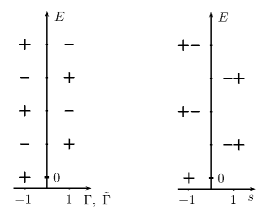
Figure 1: The spectrum of the unitary equivalent super-oscillator Hamiltonians $H$ and $\tilde{H}$ is shown on the left; the eigenvalues of the grading operators $\Gamma=\sigma_{3}$ and $\tilde{\Gamma}=\sigma_{3}\mathcal{R}$ are indicated below the corresponding states. The “$\mathbf{+}$” denotes the states with even parity, by the “$\mathbf{-}$” we marked the states with odd parity. On the right, the spectra of $\tilde{H}_{s}$, $s=\pm 1$, are shown. The degeneracy of the energy levels in each subsystem, reflected by the hidden supersymmetry, is manifested. The hidden supersymmetry is exact for $s=-1$ (there is a singlet ground state) whereas it is broken for $s=1$.

3 Special one-dimensional cases

Consider now the special cases when the transformed Hamiltonian coincides with the original one. This happens when (2.4) is the additional integral, $[H,U]=0$, of the $N=2$ supersymmetric system.

3.1 Free particle on a line

We start with the simplest case which corresponds to a free particle, $W(x)=0$, $H=P^{2}$, as it sheds a light on general features of the supersymmetric structure associated with the hidden supersymmetry in the systems we consider in what follows.

For the free particle, both pairs of the operators, (2.2) and (2.6), are integrals of motion. For $\Gamma=\sigma_{3}$ chosen as the grading operator, the $Q_{1}=\sigma_{1}P$ and $Q_{2}=-\sigma_{2}P$ are the odd, fermionic integrals, while the $\tilde{Q}_{1}=P$ and $\tilde{Q}_{2}=i\sigma_{3}\mathcal{R}P$ are the even, bosonic integrals. Accordingly, the relations (2.3) have to be supplied with the commutation relations

$$[Q_{a},\tilde{Q}_{b}]=0\,,\qquad[\tilde{Q}_{1},\tilde{Q}_{2}]=-2i\mathcal{R}\sigma_{3}H\,.$$ (3.1)

The $\Gamma=\mathcal{R}\sigma_{3}$ can be identified as the grading operator as well. The integrals (2.6) play then the role of the fermionic supercharges which satisfy the relations (2.7) (with $\tilde{H}=H$), while (2.2) are the bosonic integrals. Relations (3.1) are changed for the relations of a similar form with the duality-like replacement $Q_{a}\leftrightarrow\tilde{Q}_{a}$, $\mathcal{R}\sigma_{3}\leftrightarrow\sigma_{3}$.

If the parity operator is identified as the grading operator, $\Gamma=\mathcal{R}$, all the integrals $Q_{a}$ and $\tilde{Q}_{a}$ should be treated as fermionic supercharges. Then the anticommutation relations (2.3) and (2.7) are supplemented with the relations

$$\{Q_{a},\tilde{Q}_{b}\}=2(-1)^{a}\left(-\delta_{b1}\sigma_{a}+\delta_{b2}\epsilon_{ac}\sigma_{c}\mathcal{R}\right)H\,,$$ (3.2)

which just reflect the fact that the sigma matrices are the even integrals of motion that have to be treated as the even generators, $[\sigma_{a},\sigma_{b}]=2i\epsilon_{ab}\sigma_{3}$, in the complete nonlinear tri-supersymmetry, see [6].

The reduction of the $N=2$ supersymmetric structure generated by $H$ and $\tilde{Q}_{a}$ to the eigensubspaces $\sigma_{3}=+1$ and $\sigma_{3}=-1$ results in the bosonized supersymmetry, in which the $\Gamma=\mathcal{R}$ is identified as the grading operator, and $\tilde{Q}_{1}=P$ and $\tilde{Q}_{2}=i\mathcal{R}P$ (the sign in definition of the latter operator is irrelevant) play the role of the fermionic supercharges. The eigenstates of the $\tilde{Q}_{2}$ are $\psi_{k}(x)=\frac{1}{\sqrt{2}}e^{-i\pi/4}(e^{ikx}+ie^{-ikx})=\cos kx+\sin kx$, $\tilde{Q}_{2}\psi_{k}(x)=k\psi_{k}(x)$, $k\in(-\infty,\infty)$, cf. the eigenstates $e^{ikx}$ of $\tilde{Q}_{1}$, $\tilde{Q}_{1}e^{ikx}=ke^{ikx}$. Notice also that $\tilde{Q}_{\pm}=\tilde{Q}_{1}\pm i\tilde{Q}_{2}=P\Pi_{\pm}$ realize the Darboux transformation between the eigenstates $\cos kx$ and $\sin kx$, $k\geq 0$, of the free particle Hamiltonian $H=P^{2}$ : $\tilde{Q}_{+}\cos kx=-k\sin kx$, $\tilde{Q}_{+}\sin kx=0$, $\tilde{Q}_{-}\cos kx=0$, $\tilde{Q}_{-}\sin kx=k\cos kx$.

3.2 Dirac delta potential problem

Besides a free particle case in $\mathbb{R}^{1}$ with $W(x)=0$, let us mention another simple but nontrivial model on the line, for which the unitary transformation $U$ is the symmetry of Hamiltonian. It is given by

$$W(x)=\beta\varepsilon(x),$$ (3.3)

where $\varepsilon(x)$ is a sign function defined as $\varepsilon(x)=1$ for $x\geq 0$, and $\varepsilon(x)=-1$ for $x<0$. In this case Hamiltonian (2.1) corresponds to the $N=2$ superextended Dirac delta potential problem [14],

$$H=P^{2}+\beta^{2}+2\beta\sigma_{3}\delta(x)\,.$$ (3.4)

Since $\mathcal{R}\delta(x)\psi(x)=\delta(-x)\psi(-x)=\delta(x)\psi(x)$, the transformed Hamiltonian (2.5) coincides with the original one, (3.4). Similarly to the free particle case, $[Q_{a},\tilde{Q}_{b}]=0$.

After reduction to the eigensubspaces of the diagonal integral $\sigma_{3}$, we get two spinless one-dimensional Dirac delta potential problems with the hidden $N=2$ supersymmetry, described by

$$\tilde{H}_{s}=P^{2}+\beta^{2}+s\,2\beta\delta(x)\,,\qquad s=+1\quad{\rm or}-1\,,$$ (3.5)

$$\tilde{Q}_{1,s}=P+s\,i\beta\varepsilon(x)\mathcal{R}\,,\qquad\tilde{Q}_{2,s}=i\mathcal{R}\tilde{Q}_{1,s}\,.$$ (3.6)

The hidden supersymmetry of the spinless systems (3.5) and the tri-supersymmetric structure of the spin-$1/2$ system (3.4) were studied in [2], [6]. Here we just notice that while the Hamiltonian (3.5) is local, the both supercharges (3.6) of the hidden supersymmetry are non-local operators. For $\beta>0$ and $s=-1$ (the case of the attractive delta function potential), the system has a singlet bound state of zero energy separated by the energy gap $\beta^{2}$ from the doubly degenerate continuous (scattering) part of the spectrum, i.e. corresponding hidden supersymmetry is unbroken. For $\beta>0$, $s=+1$ (repulsive delta function potential), the system is characterized by the broken $N=2$ bosonized supersymmetry that reflects coherently the double degeneration of all the (scattering) states with $E>\beta^{2}$ in the spectrum of the system.

3.3 Bound state Aharonov-Bohm model

Consider a charged spinless particle subjected to move on a unit circle $x^{2}+y^{2}=1$ (placed in the plane $z=0$) in the presence of the magnetic field of a flux line, $B_{z}(x,y)=\epsilon_{ij}\partial_{i}A_{j}=\Phi\delta(x,y)$. The Hamiltonian of the system is given by

$$H_{\alpha}=(p_{\varphi}+\alpha)^{2}\,,$$ (3.7)

where $p_{\varphi}=-i\frac{d}{d\varphi}$, $\varphi$ is the angular variable on a unit circle, and $\alpha=-\frac{e}{2\pi c}\Phi$. This configuration corresponds to the bound state Aharonov-Bohm effect [15].

The usual $N=2$ supersymmetric extension is similar to that of the free one-dimensional particle discussed above, with the change $P\rightarrow p_{\varphi}+\alpha$. The analogue of the parity integral $\mathcal{R}$, however, does not exist for arbitrary values of the rescaled magnetic flux parameter $\alpha$.

Consider a twisted reflection operator

$$\mathcal{R}=e^{-2i\alpha\varphi}R_{\varphi}\,,$$ (3.8)

where the $R_{\varphi}$ is a reflection in $\varphi$, $R_{\varphi}\psi(\varphi)=\psi(-\varphi)$. Operator (3.8) is well defined (maps $2\pi$-periodic functions into $2\pi$-periodic ones), and commutes with the Hamiltonian (3.7) only when $\alpha$ takes integer or half-integer values.

The discrete spectrum of the system (3.7) with the energy levels $E_{l}=(l+\alpha)^{2}$, $l=0,\pm 1,\pm 2,\ldots$, which correspond to the states $e^{il\varphi}$, has a degeneration typical for the $N=2$ supersymmetry only in the same cases $\alpha=n$, or $\alpha=n+\frac{1}{2}$, $n\in\mathbb{Z}$. For $\alpha=n$, the system is unitary equivalent to the free particle on a circle case ($\alpha=0$) since $p_{\varphi}+n=\mathcal{U}_{n}p_{\varphi}\mathcal{U}_{n}^{-1}$, $\mathcal{U}_{n}=e^{-in\varphi}$. The zero-energy ground state ($l=-n$) is nondegenerate while the states with $l=k\neq-n$ and $l=-k-2n$ form a doublet of the same energy (not taking into account a double degeneration of all the levels related to the decoupled spin variables). On the contrary, for $\alpha=n+\frac{1}{2}$, all the energy levels are positive and doubly degenerate modulo the degeneration associated with the spin degrees of freedom : $E_{l}=E_{-l-2n-1}=(l+n+\frac{1}{2})^{2}\geq 1/4$.

Hence, the procedure of the special unitary transformation and subsequent reduction applies in the current system as well, where it relates the earlier observed hidden supersymmetry of the bound state AB effect [2] with the usual $N=2$ supersymmetry associated with the decoupled spin degrees of freedom.

4 Generalization to the two dimensions

Consider a charged spin-1/2 particle confined in the plane in the presence of the perpendicular magnetic field, that is described by the Pauli Hamiltonian

$$H=\mathcal{P}_{i}^{2}-\frac{e}{c}\sigma_{3}B,$$ (4.1)

where $\mathcal{P}_{i}=-i\partial_{i}-\frac{e}{c}A_{i}(\mathbf{x})$, $i=1,2$, and $B(\mathbf{x})=\epsilon_{ij}\partial_{i}A_{j}(\mathbf{x})$. For arbitrary magnetic field, such a system possess the $N=2$ supersymmetry (2.3) [with $\Gamma=\sigma_{3}$] generated by the supercharges [16]

$$Q_{1}=\sigma_{i}\mathcal{P}_{i}\,,\qquad Q_{2}=\epsilon_{ij}\sigma_{i}\mathcal{P}_{j}=i\sigma_{3}Q_{1}\,.$$ (4.2)

As we shall see, the application of this simple but formal construction of the $N=2$ supersymmetry is accompanied by the proper definition of the involved operators in the case of the planar AB effect [8].

Assume now that the magnetic field is an even function, $B(-\mathbf{x})=B(\mathbf{x})$, described in terms of the odd vector potential, $A_{i}(-\mathbf{x})=-A_{i}(\mathbf{x})$. Then the system (4.1) will have an additional, nonlocal integral

$$\mathcal{R}=\exp(i\pi L)\,,$$ (4.3)

$[H,\mathcal{R}]=0$, which corresponds to a rotation in $\pi$, where $L=-i\epsilon_{ij}x_{i}\partial_{j}$ is the orbital angular momentum. The operator (4.3) satisfies the relations $\mathcal{R}x_{i}=-x_{i}\mathcal{R}$, $\mathcal{R}^{2}=1$, and, therefore, supercharges (4.2) are the parity-odd operators, $\{\mathcal{R},Q_{a}\}=0,$ $a=1,2$. Then we can apply the analysis of Section 2 based on the special unitary transformation, in which the operator $\mathcal{R}$ is given by (4.3). The supercharges (4.2) can be obtained alternatively by making the changes $P\rightarrow\mathcal{P}_{1}$, $W\rightarrow\mathcal{P}_{2}$ in (2.2). The transformed supercharges $\tilde{Q}_{1}$ and $\tilde{Q}_{2}$ take the form

$$\tilde{Q}_{1}=\mathcal{P}_{1}-i\sigma_{3}\mathcal{R}\mathcal{P}_{2}\,,\qquad\tilde{Q}_{2}=\mathcal{P}_{2}+i\sigma_{3}\mathcal{R}\mathcal{P}_{1}\,.$$ (4.4)

Likewise in the one-dimensional systems, the operator $U$ of the unitary transformation does not commute with the Hamiltonian in general. However, there are exceptional cases, including the case of the free particle ($A_{i}=B=0$). Let us comment on this case briefly here. Following the discussion of Section 3.1, we get an explanation for the hidden $N=2$ supersymmetry of the free spinless planar particle system : it can be related to the $N=2$ supersymmetry of the spin-1/2 analog of the system via the special unitary transformation (2.4) and subsequent reduction to any of the two eigensubspaces $\sigma_{3}=+1$ or $\sigma_{3}=-1$. In the free particle case, the generators of the hidden supersymmetry,

$$\tilde{Q}_{i}=\mathcal{P}_{i}-i\sigma_{3}\mathcal{R}\epsilon_{ij}\mathcal{P}_{j},$$ (4.5)

form a two-dimensional vector with respect to to the total angular momentum $\mathcal{J}=L+\frac{1}{2}\sigma_{3}$, $[\mathcal{J},\tilde{Q}_{i}]=i\epsilon_{ij}\tilde{Q}_{j}$, in contrast with the scalar supercharges $Q_{a}$, $[\mathcal{J},Q_{a}]=0$.

Below, we shall ellaborate another two-dimensional systems where the hidden supersymmetry can be related to the standard $N=2$ supersymmetry via the unitary transformation. At first, we will analyze the two-dimensional system which is a symbiosis of the bound state AB model considered in Section 3.3, and of the free particle – the particle on the cylinder. The second model will be the celebrated planar AB model.

4.1 Aharonov-Bohm effect : the tubule model

Consider the model of a charged spin-1/2 particle on the cylinder in the presence of the AB flux along the symmetry axis ($x_{1}=0$, $-\infty<x_{2}=y<\infty$) of the cylinder. It is described by

$$H=(p_{\varphi}+\alpha)^{2}+p_{y}^{2}\,.$$ (4.6)

The (singular) magnetic field is not orthogonal to the two-dimensional surface here, but (4.6) is obtained from (4.1) by changing $\mathcal{P}_{1}\rightarrow p_{\varphi}+\alpha$, $p_{\varphi}=-i\partial/\partial\varphi$, and $\mathcal{P}_{2}\rightarrow p_{y}=-i\partial/\partial y$, and by omitting the spin term there. The supercharge integrals are obtained then from (4.2) by the same change,

$$Q_{1}=\sigma_{1}(p_{\varphi}+\alpha)+\sigma_{2}p_{y}\,,\qquad Q_{2}=i\sigma_{3}Q_{1}\,.$$ (4.7)

As in the case of the bound-state AB model, for integer and half-integer values of the rescaled magnetic flux $\alpha$, the Hamiltonian (4.6) has an additional integral

$$\mathcal{R}=e^{-2i\alpha\varphi}R_{\varphi}R_{y}\,,\qquad\alpha=n\quad{\rm or}\quad n+\frac{1}{2}\,,$$ (4.8)

where $R_{y}$ is the operator of reflection in the $y$ coordinate, $R_{y}y=-yR_{y}$. The integral (4.8) anticommutes with both supercharges $Q_{a}$. The additional, commuting with $Q_{a}$ integrals,

$$\tilde{Q}_{1}=(p_{\varphi}+\alpha)-i\sigma_{3}\mathcal{R}p_{y},\qquad\tilde{Q}_{2}=i\mathcal{R}\sigma_{3}\tilde{Q}_{1},$$ (4.9)

are obtained from (4.4) via the indicated above substitution, i.e. by applying the unitary transformation (2.4) to (4.7). The tri-supersymmetric structure associated with the three possible choices for the grading operator can be computed following the line of Section 3.1.

4.2 Planar Aharonov-Bohm effect

Consider the $N=2$ supersymmetric system that corresponds to the planar AB effect [17] for the spin$-1/2$ particle. This system is described by the Hamiltonian (4.1) with the electromagnetic potential given by

$$\vec{A}=\frac{\Phi}{2\pi}\left(-\frac{x_{2}}{x_{1}^{2}+x_{2}^{2}},\frac{x_{1}}{x_{1}^{2}+x_{2}^{2}}\right)=\frac{\Phi}{2\pi r}\left(-\sin\varphi\,,\ \cos\varphi\right)\,,$$ (4.10)

where we use the polar coordinates, $x_{1}=r\cos\varphi,\ x_{2}=r\sin\varphi$. Potential (4.10) corresponds to the singular magnetic field, $B(\mathbf{x})=\Phi\,\delta^{2}(x_{1},x_{2})$. The explicit form of the Hamiltonian is

$$\mathcal{H}_{\alpha}=-\partial^{2}_{r}-\frac{1}{r}\partial_{r}+\frac{1}{r^{2}}(-i\partial_{\varphi}+\alpha)^{2}+\alpha\frac{1}{r}\delta(r)\sigma_{3}\,,\quad\alpha=-\frac{e}{2\pi c}\Phi\,,$$ (4.11)

where we use the identity $\delta^{2}(x_{1},x_{2})=\frac{1}{\pi r}\delta(r)$ for the two dimensional Dirac delta function. Since the vector potential and magnetic field are singular functions at the point $\mathbf{x}=0$, the appropriate domains have to be specified for the Hamiltonian and supercharges (4.2) in order to keep them well defined (self-adjoint).

The AB system with the integer value of the magnetic flux is unitary equivalent to the free-particle case ($\alpha=0$) which was discussed above. In general, the relation $\mathcal{H}_{\alpha+n}=U_{n}\mathcal{H}_{\alpha}U_{n}^{-1}$ with $U_{n}=e^{-in\varphi}\mathds{1}$, where $\mathds{1}$ is the unit $2\times 2$ matrix, tells that we can assume $\alpha\in(0,1)$ without loss of generality. As it was shown in [8], the supercharges of the $N=2$ supersymmetry are well defined in two cases only, which correspond to two different self-adjoint extensions of the Hamiltonian $\mathcal{H}_{\alpha}$, denoted as $\mathcal{H}^{0}_{\alpha}$ and $\mathcal{H}^{\pi}_{\alpha}$, cf. (4.8). In other words, there are just two self-adjoint extensions of the Hamiltonian that are consistent with the $N=2$ supersymmetry. These two self-adjoint extensions,

$$\mathcal{H}^{\gamma=0}_{\alpha}=\left(\begin{array}[]{cc}H_{\alpha}^{0}&0\\ 0&H_{\alpha}^{AB}\end{array}\right)\,,\qquad\mathcal{H}^{\gamma=\pi}_{\alpha}=\left(\begin{array}[]{cc}H_{\alpha}^{AB}&0\\ 0&H_{\alpha}^{\pi}\end{array}\right),$$ (4.12)

differ in their domains. They are well defined on the locally square integrable functions, that are regular at the origin up to a single partial wave, where the singular behavior is enforced. The two component wave functions from the domain of $\mathcal{H}^{\gamma}_{\alpha}$ have to comply with the following boundary conditions :

$$\lim_{r\rightarrow 0^{+}}\Psi\sim\left(\begin{array}[]{l}(1+e^{i\gamma})2^{-\alpha}\Gamma(1-\alpha)r^{-1+\alpha}e^{-i\varphi}\\ (1-e^{i\gamma})2^{-1+\alpha}\Gamma(\alpha)r^{-\alpha}\end{array}\right).$$ (4.13)

Explicit form of the corresponding supercharges defined on the same domain is

$$Q_{1}^{\gamma}=\left(\begin{array}[]{cc}0&{\cal P}_{1}-i{\cal P}_{2}\\ {\cal P}_{1}+i{\cal P}_{2}&0\end{array}\right)\,,\qquad Q_{2}^{\gamma}=i\sigma_{3}Q_{1}^{\gamma}=\left(\begin{array}[]{cc}0&{\cal P}_{2}+i{\cal P}_{1}\\ {\cal P}_{2}-i{\cal P}_{1}&0\end{array}\right)\,.$$ (4.14)

Note that as formal differential operators, the supercharges are the same for both values of $\gamma$; however, for $\gamma=0$ and $\gamma=\pi$, their domains are different. The same is valid for the operators $H^{0}_{\alpha}$, $H^{\pi}_{\alpha}$ and $H^{AB}_{\alpha}$. For the first two, the corresponding domains admit singular (at zero) wave functions in corresponding partial waves, while the domain of $H^{AB}_{\alpha}$ includes only regular at zero functions. Therefore, the two Hamiltonian operators (4.12) describe the two different systems.

The both systems (4.12) have additional, nonlocal integral of motion (4.3) which, unlike the bound state AB effect and the related tubule model, exists for arbitrary value of the flux parameter [remind that we restrict $\alpha\in(0,\pi)$], and acts here on the angular variable as $\mathcal{R}\varphi\mathcal{R}=\varphi+\pi$.

Define the two different unitary operators,

$$U_{\pm}=\left(\begin{array}[]{cc}\Pi_{\pm}&\Pi_{\mp}\\ \Pi_{\mp}&\Pi_{\pm}\end{array}\right),$$ (4.15)

which satisfy the relations $U_{\pm}^{\dagger}=U_{\pm}$, $U_{+}^{2}=U_{-}^{2}=1$, and $U_{+}\sigma_{3}U_{+}=\sigma_{3}\mathcal{R}$, $U_{-}\sigma_{3}U_{-}=-\sigma_{3}\mathcal{R}$. Operator $U_{+}$ corresponds here to (2.4), while $U_{-}$ is obtained from it via the change $\mathcal{R}\rightarrow-\mathcal{R}$. Both $U_{\pm}$ commute with the formal Hamiltonian operator (4.11). It is necessary, however, to check how they act on the wave functions from the domain of $\mathcal{H}^{\gamma}_{\alpha}$. The $U_{+}$ respects the boundary conditions (4.13) if and only if $\gamma=\pi$, while $U_{-}$ does not alter (4.13) for $\gamma=0$. The domain of $\mathcal{H}^{\pi}_{\alpha}$ ($\mathcal{H}^{0}_{\alpha}$) is invariant with respect to $U_{+}$ ($U_{-}$), and therefore $[U_{+},\mathcal{H}^{\pi}_{\alpha}]=0$, $[U_{-},\mathcal{H}^{0}_{\alpha}]=0$. Under the unitary transformation $U_{+}$ ($U_{-}$), the Hamiltonian $\mathcal{H}^{\pi}_{\alpha}$ ($\mathcal{H}^{0}_{\alpha}$) remains the same.

Unitary transformation of the supercharges ${Q}_{a}^{\pi}$ (${Q}_{a}^{0}$) by the $U_{+}$ ($U_{-}$) gives the corresponding supercharges of the hidden $N=2$ supersymmetry. They can be written in the unified form

$$\tilde{Q}^{\gamma}_{1}=\left(\begin{array}[]{cc}\mathcal{P}_{1}+ie^{i\gamma}\mathcal{R}\mathcal{P}_{2}&0\\ 0&\mathcal{P}_{1}-ie^{i\gamma}R\mathcal{P}_{2}\end{array}\right)\,,\qquad\tilde{Q}^{\gamma}_{2}=-ie^{i\gamma}\sigma_{3}\mathcal{R}\tilde{Q}_{1}^{\gamma}\,,\qquad\gamma=0,\pi\,.$$ (4.16)

Like in the free planar particle case, the supercharges $Q_{a}^{\gamma}$ of the usual $N=2$ supersymmetry are scalars with respect to the total angular momentum ${\cal J}=L+\frac{1}{2}\sigma_{3}$, while the generators of the hidden supersymmetry, $\tilde{Q}^{\gamma}_{1}$ and $\tilde{Q}^{\gamma}_{2}$, for both $\gamma$ values form a two dimensional vector, $[{\cal J},\tilde{Q}^{\gamma}_{i}]=i\epsilon_{ij}\tilde{Q}_{j}^{\gamma}$. This also follows from the alternative representation of (4.16),

$$\tilde{Q}^{\gamma}_{i}={\cal P}_{i}\cdot\mathds{1}+ie^{i\gamma}\mathcal{R}\sigma_{3}\cdot\epsilon_{ij}{\cal P}_{j}\,,$$ (4.17)

cf. (4.4). Reduction to the eigensubspaces $\sigma_{3}=+1$ and $\sigma_{3}=-1$ produces the three different AB models for a scalar particle described by the Hamiltonians $H^{0}_{\alpha}$, $H^{\pi}_{\alpha}$ and $H^{AB}_{\alpha}$, each of which possesses the hidden supersymmetry generated by the corresponding diagonal component of (4.17). This explains the origin of the hidden supersymmetry in the AB effect for the scalar particle that was observed in [3]. Notice that the generators of the usual supersymmetry, $Q_{a}^{\gamma}$, commute with the generators $\tilde{Q}^{\gamma}_{i}$ of the hidden supersymmetry, $[{Q}_{a}^{\gamma},\tilde{Q}^{\gamma}_{i}]=0$, for both $\gamma=0$ and $\gamma=\pi$.

The tri-supersymmetry of the system, associated with three alternative grading operators and discussed in [8], can be obtained in the same vain as in Section 3.1.

5 Unusual $N=2$ supersymmetry in the three dimensions

Consider a three-dimensional spin-$1/2$ particle in magnetic field $B_{i}(\mathbf{x})=\epsilon_{ijk}\partial_{j}A_{k}(\mathbf{x})$. The system is described by the Hamiltonian,

$$H=P_{i}^{2}+\sigma_{i}B_{i}\,,$$ (5.1)

and possesses the $N=1$ supersymmetry described by the supercharge

$$\tilde{Q}_{1}=P_{i}\sigma_{i}\,,$$ (5.2)

$\tilde{Q}_{1}^{2}=H$. Here $P_{i}=-i\partial_{i}-\frac{e}{c}A_{i}(\mathbf{x})$, and summation in $i=1,2,3$ is assumed.

The $N=1$ supersymmetry can be extended to the artificial $N=2$ supersymmetry by introducing the “isospin” degrees of freedom described by another set of Pauli matrices, which we denote by $\Sigma_{l}$, $l=1,2,3$, and by defining

$$Q_{1}=\Sigma_{1}\tilde{Q}_{1},\qquad Q_{2}=\Sigma_{2}\tilde{Q}_{1}=i\Sigma_{3}Q_{1}\,.$$ (5.3)

Suppose now that the vector potential $\mathbf{A}(\mathbf{x})$ is a parity odd function, $A_{i}(-\mathbf{x})=-A_{i}(\mathbf{x})$. Then magnetic field is an even function, the parity operator $\mathcal{R}$, $\mathcal{R}x_{i}=-x_{i}\mathcal{R}$, anticommutes with the supercharges $Q_{a}$, and commutes with $H$. The structure we have obtained is similar to the supersymmetric structure of the one-dimensional free particle with the $\tilde{Q}_{1}$ and $\Sigma_{l}$ corresponding here to the $P$ and $\sigma_{i}$ in the latter system.

Realizing the unitary transformation (2.4) (with $\sigma_{1}$ substituted for $\Sigma_{1}$), and subsequently reducing the system to the eigensubspace $\Sigma_{3}=+1$, we find that the system (5.1) is described by the $N=2$ supersymmetry with the supercharges (5.2) and $\tilde{Q}_{2}=i\mathcal{R}\tilde{Q}_{1}$, for which the parity $\mathcal{R}$ plays a role of the grading operator. This shows that the unusual $N=2$ supersymmetry of the system (5.1) with odd vector potential, observed earlier in [9, 10], has the same nature as the hidden supersymmetry of the free particle.

6 Discussion

Up to now, our discussion was restricted to the supersymmetries generated by the time-independent operators. In the case of the spin-1/2 free particle and the planar Aharonov-Bohm model, the $N=2$ supersymmetry can be extended to the superconformal symmetry, supplying the Hamiltonian with bosonic generators of the dilatations $D$ and special conformal transformations $K$. Their commutator with the the supercharges $Q_{a}$ generate the additional odd integrals $S_{a}$, that depend explicitly on time [8, 18], $S_{a}=i[K,Q_{a}]$. Since the indicated bosonic generators $K$ and $D$ are diagonal operators and commute with the reflection operator $\mathcal{R}$, they are invariant with respect to the unitary transformation $U$. This is not the case for $S_{a}$, which is transformed into the diagonal time-dependent symmetry $\tilde{S}_{a}=U\,S_{a}\,U^{-1}$. The subsequent reduction to the eigensubspaces $\sigma_{3}=+1$ and $\sigma_{3}=-1$ gives rise to the hidden superconformal symmetry of the scalar free particle [11] and for the spinless AB effect [3] and, therefore, clarifies its origin.

In all the systems we considered, the generators of the usual $N=2$ supersymmetry commute with the generators of the hidden supersymmetry. This means that if one of the generators of the usual supersymmetry is identified as a first order Hamiltonian like that in the massless Dirac particle case [19, 20], such a first order system will possess a hidden $N=2$ supersymmetry. This observation can be applied in the condensed matter systems described by the Dirac-Weyl equation, and will be elaborated elsewhere.

We have explained the origin of the hidden supersymmetry of some quantum mechanical systems, where the corresponding supercharges are the first order (nonlocal) differential operators. Notice that this construction, based on the nonlocal unitary Foldy-Wouthuysen transformation, is completely different from that in [21], where the hidden supersymmetry is described by local supercharges. The open question is then whether a usual $N=2$ linear or nonlinear supersymmetry of the quantum periodic finite-gap systems [22, 23, 24, 25, 26] could be related in a similar way, via a nonlocal unitary transformation, to the hidden supersymmetry associated with the higher order nontrivial Lax operators [7].

Acknowledgements. The work of MSP has been partially supported by FONDECYT Grant 1095027, Chile and by Spanish Ministerio de Educación under Project SAB2009-0181 (sabbatical grant). LMN has been partially supported by the Spanish Ministerio de Ciencia e Innovación (Project MTM2009-10751) and Junta de Castilla y León (Excellence Project GR224). VJ was supported by the Czech Ministry of Education, Youth and Sports within the project LC06002.

References

- [1] M. S. Plyushchay, Annals Phys. 245 (1996) 339 [arXiv:hep-th/9601116]; J. Gamboa, M. Plyushchay and J. Zanelli, Nucl. Phys. B 543 (1999) 447 [arXiv:hep-th/9808062]; M. Plyushchay, Int. J. Mod. Phys. A 15 (2000) 3679 [arXiv:hep-th/9903130].
- [2] F. Correa and M. S. Plyushchay, Annals Phys. 322 (2007) 2493 [arXiv:hep-th/0605104].
- [3] F. Correa, H. Falomir, V. Jakubský and M. S. Plyushchay, J. Phys. A 43 (2010) 075202 [arXiv:0906.4055 [hep-th]].
- [4] F. Correa, L. M. Nieto and M. S. Plyushchay, Phys. Lett. B 644 (2007) 94 [arXiv:hep-th/0608096].
- [5] F. Correa, V. Jakubský and M. S. Plyushchay, Annals Phys. 324 (2009) 1078 [arXiv:0809.2854 [hep-th]].
- [6] F. Correa, L. M. Nieto and M. S. Plyushchay, Phys. Lett. B 659 (2008) 746 [arXiv:0707.1393 [hep-th]].
- [7] F. Correa, V. Jakubský, L. M. Nieto and M. S. Plyushchay, Phys. Rev. Lett. 101 (2008) 030403 [arXiv:0801.1671 [hep-th]]; F. Correa, V. Jakubský and M. S. Plyushchay, J. Phys. A 41 (2008) 485303 [arXiv:0806.1614 [hep-th]].
- [8] F. Correa, H. Falomir, V. Jakubský and M. S. Plyushchay, arXiv:1003.1434 [hep-th], Annals Phys., to appear.
- [9] L. E. Gendenshtein, JETP Lett. 39 (1984) 280 [Pisma Zh. Eksp. Teor. Fiz. 39 (1984) 234].
- [10] L. E. Gendenshtein and I. V. Krive, Sov. Phys. Usp. 28 (1985) 645 [Usp. Fiz. Nauk 146 (1985) 553].
- [11] F. Correa, M. A. del Olmo and M. S. Plyushchay, Phys. Lett. B 628 (2005) 157 [arXiv:hep-th/0508223].
- [12] E. Witten, Nucl. Phys. B 188 (1981) 513.
- [13] F. Cooper, A. Khare and U. Sukhatme, Phys. Rept. 251 (1995) 267 [arXiv:hep-th/9405029].
- [14] L. J. Boya, Eur. J. Phys. 9 (1988) 140.
- [15] M. Peshkin and A. Tonomura, The Aharonov-Bohm effect, Springer-Verlag (1989).
- [16] Y. Aharonov and A. Casher, Phys. Rev. A 19 (1979) 2461.
- [17] Y. Aharonov and D. Bohm, Phys. Rev. 115 (1959) 485.
- [18] P. A. Horvathy, Rev. Math. Phys. 18 (2006) 329 [arXiv:hep-th/0512233].
- [19] R. Jackiw, Phys. Rev. D 29 (1984) 2375 [Erratum-ibid. D 33 (1986) 2500].
- [20] F. Correa, G. V. Dunne and M. S. Plyushchay, Annals Phys. 324 (2009) 2522 [arXiv:0904.2768 [hep-th]].
- [21] A. A. Andrianov, F. Cannata, M. V. Ioffe and D. Nishnianidze, Phys. Lett. A 266 (2000) 341 [arXiv:quant-ph/9902057]; A. A. Andrianov and A. V. Sokolov, Nucl. Phys. B 660 (2003) 25 [arXiv:hep-th/0301062]; SIGMA 5 (2009) 064 [arXiv:0906.0549 [hep-th]].
- [22] H. W. Braden and A. J. Macfarlane, J. Phys. A 18 (1985) 3151.
- [23] G. V. Dunne and J. Feinberg, Phys. Rev. D 57 (1998) 1271 [arXiv:hep-th/9706012].
- [24] A. Khare and U. Sukhatme, J. Math. Phys. 40 (1999) 5473 [arXiv:quant-ph/9906044].
- [25] D. J. Fernandez, J. Negro and L. M. Nieto, Phys. Lett. A 275 (2000) 338.
- [26] D. J. Fernandez, B. Mielnik, O. Rosas-Ortiz and B. F. Samsonov, Phys. Lett. A 294 (2002) 168 [arXiv:quant-ph/0302204].