Abstract

This paper tackles the problem of image deconvolution with joint estimation of PSF parameters and hyperparameters. Within a Bayesian framework, the solution is inferred via a global a posteriori law for unknown parameters and object. The estimate is chosen as the posterior mean, numerically calculated by means of a Monte-Carlo Markov chain algorithm. The estimates are efficiently computed in the Fourier domain and the effectiveness of the method is shown on simulated examples. Results show precise estimates for PSF parameters and hyperparameters as well as precise image estimates including restoration of high-frequencies and spatial details, within a global and coherent approach.

OCIS codes: 100.1830, 100.3020, 100.3190, 150.1488

1 Introduction

Image deconvolution has been an active research field for several decades and recent contributions can be found in papers such as [1, 2, 3]. Examples of application are medical imaging, astronomy, nondestructive testing and more generally imagery problems. In these applications, degradations induced by the observation instrument limit the data resolution while the need of precise interpretation can be of major importance. For example, this is particularly critical for long-wavelength astronomy (see e.g., [4]). In addition, the development of a high quality instrumentation system must rationally be completed by an equivalent level of quality in the development of data processing methods. Moreover, even for poor performance systems, the restoration method can be used to bypass instrument limitations.

When the deconvolution problem is ill-posed a possible solution relies on regularization, i.e., introduction of information in addition to the data and the acquisition model [5, 6]. As a consequence of regularization, deconvolution methods are specific to the class of image in accordance with the introduced information. From this standpoint, the present paper is dedicated to relatively smooth images encountered for numerous applications in imagery [4, 7, 8]. The second order consequence of ill-posedness and regularization is the need to balance the compromise between different sources of information.

In the Bayesian approach [1, 9], information about unknowns is introduced by means of probabilistic models. Once these models are designed, the next step is to build the a posteriori law, given the measured data. The solution is then defined as a representative point of this law and the two most classical are (1) the maximizer, and (2) the mean. From a computational standpoint, the first leads to a numerical optimization problem and the latter leads to a numerical integration problem. However, the resulting estimate depends on two sets of variables in addition to the data.

1. Firstly, the estimate naturally depends on the response of the instrument at work, namely the point spread function (PSF). The literature is predominantly devoted to deconvolution in the case of known PSF. On the contrary, the present paper is devoted to the case of unknown or poorly known PSF and there are two main strategies to tackle its estimation from the available data set (without extra measurements).

   • In most practical cases, the instrument can be modeled using physical operating description. It is thus possible to find the equation for the PSF, at least in a first approximation. This equation is usually driven by a relatively small number of parameters. It is a common case in optical imaging where a Gaussian-shaped PSF is often used [10]. It is also the case in other fields: interferometry [11], magnetic resonance force microscopy [12], fluorescence microscopy [13],…Nevertheless, in real experiments, the parameter values are unknown or imperfectly known and need to be estimated or adjusted in addition to the image of interest: the question is namely myopic deconvolution.

   • The second strategy forbears the use of the parametric PSF deduced from the physical analysis and the PSF then naturally appears in a non-parametric form. Practically, the non-parametric PSF is unknown or imperfectly known and needs to be estimated in addition to the image of interest: the question is referred to as blind deconvolution for example in interferometry [14, 15, 16, 17].

   From an inference point of view, the difficulty of both myopic and blind problems lies in the possible lack of information resulting in ambiguity between image and PSF, even in the noiseless case. In order to resolve the ambiguity, information must be added [3, 18] and it is crucial to make inquiries based on any available source of information. To this end, the knowledge of the parametric PSF represents a precious means to structure the problem and possibly resolve the degeneracies. Moreover, due to instrument design process, a nominal value as well as an uncertainty are usually available for the PSF parameters.

   In addition, from a practical and algorithmic standpoint, the myopic case, i.e., the case of parametric PSF, is often more difficult due to the non-linear dependence of the observation model with respect to the PSF parameters. On the contrary, the blind case, i.e., the case of non-parametric PSF, yields a simpler practical and algorithmic problem since the observation model remains linear w.r.t. the unknown elements given the object.

   Despite the superior technical difficulty, the present paper is devoted to the myopic format since it is expected to be more efficient than the blind format from an information standpoint. Moreover, the blind case has been extensively studied and a large amount of paper is available [19, 20, 21], while the myopic case has been less investigated, though it is of major importance.

2. Secondly, the solution depends on the probability law parameters named hyperparameters (means, variances, parameters of correlation matrix,…). These parameters adjust the shape of the laws and in the same time they tune the compromise between the information provided by the a priori and the information provided by the data. In real experiments, their values are unknown and need to be estimated: the question is namely unsupervised deconvolution.

For both families of parameters (PSF parameters and hyperparameters), two approaches are available. In the first one, the parameter values are empirically tuned or estimated in a preliminary step (with Maximum Likelihood [7] or calibration [22] for example), then the values are used in a second step devoted to image restoration given the parameters. In the second one, the parameters and the object are jointly estimated [19, 2].

For the myopic problem, Jalobeanu et al. [23] address the case of a symmetric Gaussian PSF. The width parameter and the noise variance are estimated in a preliminary step by Maximum-Likelihood. A recent paper [24] addresses the estimation of a Gaussian blur parameter, as in our experiment, with an empirical method. They found the Gaussian blur parameter by minimizing the absolute derivatives of the restored images Laplacian.

The present paper addresses the myopic and unsupervised deconvolution problem. We propose a new method that jointly estimates the PSF parameters, the hyperparameters, and the image of interest. It is built in a coherent and global framework based on an extended a posteriori law for all the unknown variables. The posterior law is obtained via the Bayes rule, founded on a priori laws: Gaussian for image and noise, uniform for PSF parameters and gamma or Jeffreys for hyperparameters.

Regarding the image prior law, we have paid special attention to the parametrization of the covariance matrix in order to facilitate law manipulations such as integration, conditioning or hyperparameter estimation. The possible degeneracy of the a posteriori law in some limit cases is also studied.

The estimate is chosen as the mean of the posterior law and is computed using Monte-Carlo simulations. To this end, Monte-Carlo Markov chain (MCMC) algorithms [25] enable to draw samples from the posterior distribution despite its complexity and especially the non-linear dependence w.r.t. the PSF parameters.

The paper is structured in the following manner. Sec. 2 presents the notations and states the problem. The three following sections describe our methodology: firstly the Bayesian probabilistic models are detailed in Sec. 3; then a proper posterior law is established in Sec. 4; an MCMC algorithm to compute the estimate is described in Sec. 5. Numerical results are shown in Sec. 6. Finally, Sec. 7 is devoted to conclusion and perspectives.

2 Notations and convolution model

Consider $N$ pixels real square images represented in lexicographic order by vector ${\mathb{x}}\in\mathds{R}^{N}$, with generic elements $x_{n}$. The forward model writes

$${\mathb{y}}={\mathb{H}}_{\mathb{w}}\,{\mathb{x}}+{\boldsymbol{\epsilon}}$$ (1)

where ${\mathb{y}}\in\mathds{R}^{N}$ is the vector of data, ${\mathb{H}}_{\mathb{w}}$ a convolution matrix, ${\mathb{x}}$ the image of interest and ${\boldsymbol{\epsilon}}$ the modelization errors or the noise. Vector ${\mathb{w}}\in\mathds{R}^{P}$ stands for the PSF parameters, such as width or orientation of a Gaussian PSF.

The matrix ${\mathb{H}}_{\mathb{w}}$ is block-circulant with circulant-block (BCCB) for computational efficiency of the convolution in the Fourier space. The diagonalization [26] of ${\mathb{H}}_{\mathb{w}}$ writes ${\boldsymbol{\Lambda}}_{{\mathb{H}}}={\mathb{F}}{\mathb{H}}_{\mathb{w}}{\mathb{F}}^{\dagger}$ where ${\mathb{F}}$ is the unitary Fourier matrix and ${\dagger}$ is the transpose conjugate symbol. The convolution, in the Fourier space, is then

$$\overset{\kern-3.30002pt~{}_{\circ}}{{\mathb{y}}}={\boldsymbol{\Lambda}}_{{\mathb{H}}}\,\overset{\kern-3.30002pt~{}_{\circ}}{{\mathb{x}}}+\overset{\kern-3.30002pt~{}_{\circ}}{{\boldsymbol{\epsilon}}}$$ (2)

where $\overset{\kern-3.30002pt~{}_{\circ}}{{\mathb{x}}}={\mathb{F}}{\mathb{x}}$, $\overset{\kern-3.30002pt~{}_{\circ}}{{\mathb{y}}}={\mathb{F}}{\mathb{y}}$ and $\overset{\kern-3.30002pt~{}_{\circ}}{{\boldsymbol{\epsilon}}}={\mathb{F}}{\boldsymbol{\epsilon}}$ are the 2D discrete Fourier transform (dft-2d) of image, data and noise, respectively.

Since ${\boldsymbol{\Lambda}}_{{\mathb{H}}}$ is diagonal, the convolution is computed with a term-wise product in the Fourier space. There is a strict equivalence between a description in spatial domain (Eq. (1)) and in Fourier domain (Eq. (2)). Consequently, for coherent description and computational efficiency, all the developments are equally done in the spatial space or in the Fourier space.

For notational convenience, let us introduce the component at null-frequency $\overset{\kern-3.30002pt~{}_{\circ}}{x}_{0}\in\mathds{R}$ and the vector of component at non-null frequencies $\overset{\kern-3.30002pt~{}_{\circ}}{{\mathb{x}}}_{*}\in\mathds{C}^{N-1}$ so that the whole set of components writes $\overset{\kern-3.30002pt~{}_{\circ}}{{\mathb{x}}}=[\overset{\kern-3.30002pt~{}_{\circ}}{x}_{0},\overset{\kern-3.30002pt~{}_{\circ}}{{\mathb{x}}}_{*}]$.

Let us note $\mathds{1}$ the vector of $N$ components equal to $1/N$, so that $\mathds{1}^{\mathrm{t}}{\mathb{x}}$ is the empirical mean level of the image. The Fourier components are the $\overset{\kern-3.30002pt~{}_{\circ}}{\mathds{1}}_{n}$ and we have: $\overset{\kern-3.30002pt~{}_{\circ}}{\mathds{1}}_{0}=1$ and $\overset{\kern-3.30002pt~{}_{\circ}}{\mathds{1}}_{n}=0$ for $n\neq 0$. Moreover, ${\boldsymbol{\Lambda}}_{\mathds{1}}={\mathb{F}}\mathds{1}\mathds{1}^{\mathrm{t}}{\mathb{F}}^{\dagger}$ is a diagonal matrix with only one non-null coefficient at null frequency.

3 Bayesian probabilistic model

This section presents the prior law for each set of parameters. Regarding the image of interest, in order to account for smoothness, the law introduces high-frequency penalization through a differential operator on the pixel. A conjugate law is proposed for the hyperparameters and a uniform law is considered for the PSF parameters.

Moreover, we have paid a special attention to the image prior law parametrization. In the next section we present several parametrization in order to facilitate law manipulations such as integration, conditioning or hyperparameter estimation. Moreover, the correlation matrix of the image law may become singular in some limit cases resulting in a degenerated prior law (when $p({\mathb{x}})=0$ for all ${\mathb{x}}\in\mathds{R}^{N}$). Based on this parametrization, Sec. 4 studies the degeneracy of the posterior in relation with the parameters of the prior law.

3.A Image prior law

The probability law for the image is a Gaussian field with a given precision matrix ${\mathb{P}}$ parametrized by a vector ${\boldsymbol{\gamma}}$. The pdf reads

$$p({\mathb{x}}|{\boldsymbol{\gamma}})=(2\pi)^{-N/2}\det[{\mathb{P}}]^{1/2}\,\exp\left[-\frac{1}{2}\,{\mathb{x}}^{\mathrm{t}}{\mathb{P}}{\mathb{x}}\right]\,.$$ (3)

For computational efficiency, the precision matrix is designed (or approximated) in a toroidal manner, and it is diagonal in the Fourier domain ${\boldsymbol{\Lambda}}_{\mathb{P}}={\mathb{F}}{\mathb{P}}{\mathb{F}}^{\dagger}$. Thus, the law for ${\mathb{x}}$ also writes

$$p({\mathb{x}}|{\boldsymbol{\gamma}}) =(2\pi)^{-N/2}\det[{\mathb{F}}]\det[{\boldsymbol{\Lambda}}_{\mathb{P}}]^{1/2}\det[{\mathb{F}}^{{\dagger}}]\,\exp\left[-\frac{1}{2}{\mathb{x}}^{t}{\mathb{F}}^{{\dagger}}{\boldsymbol{\Lambda}}_{\mathb{P}}{\mathb{F}}{\mathb{x}}\right]$$ (4)

$$=(2\pi)^{-N/2}\det[{\boldsymbol{\Lambda}}_{\mathb{P}}]^{1/2}\,\exp\left[-\frac{1}{2}\overset{\kern-3.30002pt~{}_{\circ}}{{\mathb{x}}}^{\dagger}{\boldsymbol{\Lambda}}_{\mathb{P}}\overset{\kern-3.30002pt~{}_{\circ}}{{\mathb{x}}}\right]$$ (5)

and it is sometimes referred to [27] as a Whittle approximation (see also [28, p.133]) for the Gaussian law. The filter obtained for fixed hyperparameters is also the Wiener-Hunt filter [29], as described in Sec. 5.A.

This paper focuses on smooth images, thus on positive correlation between pixels. It is introduced by high-frequencies penalty using any circulant differential operator: $p$-th differences between pixels, Laplacian, Sobel…The differential operator is denoted by ${\mathb{D}}$ and its diagonalized form by ${\boldsymbol{\Lambda}}_{{\mathb{D}}}={\mathb{F}}{\mathb{D}}{\mathb{F}}^{\dagger}$. Then, the precision matrix writes ${\mathb{P}}=\gamma_{1}{\mathb{D}}^{\mathrm{t}}{\mathb{D}}$ and its Fourier counterpart writes

$${\boldsymbol{\Lambda}}_{\mathb{P}}=\gamma_{1}{\boldsymbol{\Lambda}}_{{\mathb{D}}}^{\dagger}{\boldsymbol{\Lambda}}_{{\mathb{D}}}={\mathrm{diag}}\left(0,\gamma_{1}|\overset{\kern-3.30002pt~{}_{\circ}}{d}_{1}|^{2},\ldots,\gamma_{1}|\overset{\kern-3.30002pt~{}_{\circ}}{d}_{N-1}|^{2}\right)$$ (6)

where $\gamma_{1}$ is a positive scale factor, ${\mathrm{diag}}$ builds a diagonal matrix from elementary components and $\overset{\kern-3.30002pt~{}_{\circ}}{d}_{n}$ is the $n$-th dft-2d coefficient of ${\mathb{D}}$.

Under this parametrization of ${\mathb{P}}$, the first eigenvalue is equal to zero corresponding to the absence of penalty for the null frequency $\overset{\kern-3.30002pt~{}_{\circ}}{x}_{0}$, i.e., no information accounted for about the empirical mean level of the image. As a consequence, the determinant vanishes $\det[{\mathb{P}}]=0$ resulting in a degenerated prior. To manage this difficulty, several approaches have been proposed.

Some authors [2, 30] still use this prior despite its degeneracy and this approach can be analyzed in two ways.

1. On the one hand, it can be seen as a non-degenerated law for $\overset{\kern-3.30002pt~{}_{\circ}}{{\mathb{x}}}_{*}$, the set of non-null frequency components only. In this format, the prior does not affect any probability to the null frequency component and the Bayes rule does not apply to this component. Thus, this strategy yields an incomplete posterior law, since the null frequency is not embedded in the methodology.

2. On the other hand, it can be seen as a degenerated prior for the whole set of frequencies. The application of the Bayes rule is then somewhat confusing due to degeneracy. In this format, the posterior law cannot be guaranteed to remain non-degenerated.

Anyway, none of the two standpoints yields a posterior law that is both non-degenerated and addressing the whole set of frequencies.

An alternative parametrization relies on the energy of ${\mathb{x}}$. An extra term ${\gamma_{0}}{\mathb{I}}$, tuned by $\gamma_{0}>0$, in the precision matrix [31], introduces information for all the frequencies including $\overset{\kern-3.30002pt~{}_{\circ}}{x}_{0}$. The precision matrix writes

$$\Lambda_{\mathb{P}} =\gamma_{0}{\mathb{I}}+\gamma_{1}{\boldsymbol{\Lambda}}_{{\mathb{D}}}^{\dagger}{\boldsymbol{\Lambda}}_{{\mathb{D}}}$$

$$={\mathrm{diag}}\left(\gamma_{0},\gamma_{0}+\gamma_{1}|\overset{\kern-3.30002pt~{}_{\circ}}{d}_{1}|^{2},\ldots,\gamma_{0}+\gamma_{1}|\overset{\kern-3.30002pt~{}_{\circ}}{d}_{N-1}|^{2}\right)$$ (7)

with a determinant

$$\det[\Lambda_{\mathb{P}}]=\prod_{n=0}^{N-1}\left(\gamma_{0}+\gamma_{1}|\overset{\kern-3.30002pt~{}_{\circ}}{d}_{n}|^{2}\right).$$ (8)

The obtained Gaussian prior is not degenerated and undoubtedly leads to a proper posterior. Nevertheless, the determinant Eq. (8) is not separable in $\gamma_{0}$ and $\gamma_{1}$. Consequently, the conditional posterior for these parameters is not a classical law and future development will be more difficult. Moreover, the non-null frequencies $\overset{\kern-3.30002pt~{}_{\circ}}{{\mathb{x}}}_{*}$ are controlled by two parameters $\gamma_{0}$ and $\gamma_{1}$

$$p(\overset{\kern-3.30002pt~{}_{\circ}}{{\mathb{x}}}|\gamma_{0},\gamma_{1})=p(\overset{\kern-3.30002pt~{}_{\circ}}{x}_{0}|\gamma_{0})p(\overset{\kern-3.30002pt~{}_{\circ}}{{\mathb{x}}}_{*}|\gamma_{0},\gamma_{1}).$$ (9)

The proposed approach to manage the degeneracy relies on the addition of a term for the null frequency only ${\boldsymbol{\Lambda}}_{\mathds{1}}={\mathrm{diag}}\left(1,0,\ldots,0\right)$

$$\Lambda_{\mathb{P}} =\gamma_{0}{\boldsymbol{\Lambda}}_{\mathds{1}}^{\dagger}{\boldsymbol{\Lambda}}_{\mathds{1}}+\gamma_{1}{\boldsymbol{\Lambda}}_{{\mathb{D}}}^{\dagger}{\boldsymbol{\Lambda}}_{{\mathb{D}}}.$$ (10)

$$={\mathrm{diag}}\left(\gamma_{0},\gamma_{1}|\overset{\kern-3.30002pt~{}_{\circ}}{d}_{1}|^{2},\ldots,\gamma_{1}|\overset{\kern-3.30002pt~{}_{\circ}}{d}_{N-1}|^{2}\right)\,.$$

The determinant has a separable expression

$$\det[\Lambda_{\mathb{P}}] =\gamma_{0}\gamma_{1}^{N-1}\prod_{n=1}^{N-1}|\overset{\kern-3.30002pt~{}_{\circ}}{d}_{n}|^{2}\,,$$ (11)

i.e., the precision parameters have been factorized. In addition, each parameter controls a different set of frequencies:

$$p(\overset{\kern-3.30002pt~{}_{\circ}}{{\mathb{x}}}|\gamma_{0},\gamma_{1})=p(\overset{\kern-3.30002pt~{}_{\circ}}{x}_{0}|\gamma_{0})p(\overset{\kern-3.30002pt~{}_{\circ}}{{\mathb{x}}}_{*}|\gamma_{1})\,,$$

$\gamma_{0}$ drives the empirical mean level of the image $\overset{\kern-3.30002pt~{}_{\circ}}{x}_{0}$ and $\gamma_{1}$ drives the smoothness $\overset{\kern-3.30002pt~{}_{\circ}}{{\mathb{x}}}_{*}$ of the image. With the Fourier precision structure of Eq. (10), we have the non-degenerated prior law for the image that addresses separately all the frequencies with a factorized partition function w.r.t. $(\gamma_{0},\gamma_{1})$

$$p({\mathb{x}}|\gamma_{0},\gamma_{1})=(2\pi)^{-N/2}\prod_{n=1}^{N-1}|\overset{\kern-3.30002pt~{}_{\circ}}{d}_{n}|\,\gamma_{0}^{1/2}\gamma_{1}^{(N-1)/2}\exp\left[-\frac{\gamma_{0}}{2}\|\overset{\kern-3.30002pt~{}_{\circ}}{x}_{0}\|^{2}-\frac{\gamma_{1}}{2}\|{\boldsymbol{\Lambda}}_{{\mathb{D}}*}\overset{\kern-3.30002pt~{}_{\circ}}{{\mathb{x}}}_{*}\|^{2}\right].$$ (12)

where ${\boldsymbol{\Lambda}}_{{\mathb{D}}*}$ is obtained from ${\boldsymbol{\Lambda}}_{{\mathb{D}}}$ without the first line and column. The next step is to write the a priori law for the noise in an explicit form and the other parameters, including the law parameters ${\boldsymbol{\gamma}}$ and the instrument parameters ${\mathb{w}}$.

3.B Noise and data laws

From a methodological standpoint, any statistic can be included for errors (measurement and model errors). It is possible to account for correlations in the error process or to account for a non-Gaussian law, e.g., Laplacian law, generalized Gaussian law, or other laws based on robust norm,…In the present paper, the noise is modeled as zero-mean white Gaussian vector with unknown precision parameter $\gamma_{\epsilon}$

$$p({\boldsymbol{\epsilon}}|\gamma_{\epsilon})=\left(2\pi\right)^{-N/2}\gamma_{\epsilon}^{N/2}\exp\left[-\frac{\gamma_{\epsilon}}{2}\|{\boldsymbol{\epsilon}}\|^{2}\right].$$ (13)

Consequently, the likelihood for the parameters given the observed data writes

$$p({\mathb{y}}|{\mathb{x}},\gamma_{\epsilon},{\mathb{w}})=(2\pi)^{-N/2}\gamma_{\epsilon}^{N/2}\exp\left[-\frac{\gamma_{\epsilon}}{2}\|{\mathb{y}}-{\mathb{H}}_{{\mathb{w}}}{\mathb{x}}\|^{2}\right].$$ (14)

It naturally depends on the image ${\mathb{x}}$, on the noise parameter $\gamma_{\epsilon}$ and on the PSF parameters ${\mathb{w}}$ embedded in ${\mathb{H}}_{{\mathb{w}}}$. It clearly involves a least squares discrepancy that can be rewritten in the Fourier domain: $\|{\mathb{y}}-{\mathb{H}}_{{\mathb{w}}}{\mathb{x}}\|^{2}=\|\overset{\kern-3.30002pt~{}_{\circ}}{{\mathb{y}}}-{\boldsymbol{\Lambda}}_{{\mathb{H}}}\overset{\kern-3.30002pt~{}_{\circ}}{{\mathb{x}}}\|^{2}$.

3.C Hyperparameters law

A classical choice for hyperparameter law relies on conjugate prior [32]: the conditional posterior for the hyperparameters is in the same family as its prior. It results in practical and algorithmic facilities: update of the laws amounts to update of a small number of parameters.

The three parameters $\gamma_{0}$, $\gamma_{1}$ and $\gamma_{\epsilon}$ are precision parameters of Gaussian laws Eq. (12) and (14) and a conjugate law for these parameters is the Gamma law (see Appendix B). Given parameters $(\alpha_{i},\beta_{i})$, for $i=0$, 1 or $\epsilon$, the pdf reads

$$p(\gamma_{i})=\frac{1}{\beta_{i}^{\alpha_{i}}\Gamma(\alpha_{i})}\gamma_{i}^{\alpha_{i}-1}\exp\left(-\gamma_{i}/\beta_{i}\right),\forall\gamma_{i}\in[0,+\infty[$$ (15)

In addition to computational efficiency, the law allows for non-informative priors. With specific parameter values, one obtains two improper non-informative prior : the Jeffreys’ law $p(\gamma)=1/\gamma$ and the uniform law $p(\gamma)={\mathcal{U}}_{[0,+\infty[}(\gamma)$ with $(\alpha_{i},\beta_{i})$ set to $(0,+\infty)$ and $(1,+\infty)$, respectively. Jeffreys’ law is a classical law for the precisions and is considered as non-informative [33]. This law is also invariant to power transformations: the law of $\gamma^{n}$ [33, 34] is also a Jeffreys’ law. For these reasons development is done using the Jeffreys’ law.

3.D PSF parameters law

Regarding the PSF parameters ${\mathb{w}}$, we consider that the instrument design process or a physical study provides a nominal value $\overline{{\mathb{w}}}$ with uncertainty ${\boldsymbol{\delta}}$, that is to say ${\mathb{w}}\in[\overline{{\mathb{w}}}-{\boldsymbol{\delta}}~{},~{}\overline{{\mathb{w}}}+{\boldsymbol{\delta}}]$. The ”Principle of Insufficient Reason” [33] leads to a uniform prior on this interval

$$p({\mathb{w}})={\mathcal{U}}_{\overline{{\mathb{w}}},{\boldsymbol{\delta}}}({\mathb{w}})$$ (16)

where ${\mathcal{U}}_{\overline{{\mathb{w}}},{\boldsymbol{\delta}}}$ is a uniform pdf on $[\overline{{\mathb{w}}}-{\boldsymbol{\delta}}~{},~{}\overline{{\mathb{w}}}+{\boldsymbol{\delta}}]$. Nevertheless, within the proposed framework, the choice is not limited and other laws, such as Gaussian, are possible. Anyway other choices do not allow easier computation because of the non-linear dependency of the observation model w.r.t. PSF parameters.

4 Proper posterior law

At this point, the prior law of each parameter is available: the PSF parameters, the hyperparameters and the image. Thus, the joint law for all the parameters is built by multiplying the likelihood Eq. (14) and the a priori laws Eq. (12), (15) and (16)

$$p(\overset{\kern-3.30002pt~{}_{\circ}}{{\mathb{x}}},\gamma_{\epsilon},\gamma_{0},\gamma_{1},{\mathb{w}},\overset{\kern-3.30002pt~{}_{\circ}}{{\mathb{y}}})=p(\overset{\kern-3.30002pt~{}_{\circ}}{{\mathb{y}}}|\overset{\kern-3.30002pt~{}_{\circ}}{{\mathb{x}}},\gamma_{\epsilon},{\mathb{w}})p(\overset{\kern-3.30002pt~{}_{\circ}}{{\mathb{x}}}|\gamma_{0},\gamma_{1})p(\gamma_{\epsilon})p(\gamma_{0})p(\gamma_{1})p({\mathb{w}})$$ (17)

and explicitly

$$p(\overset{\kern-3.30002pt~{}_{\circ}}{{\mathb{x}}},\gamma_{\epsilon},\gamma_{0},\gamma_{1},{\mathb{w}},\overset{\kern-3.30002pt~{}_{\circ}}{{\mathb{y}}})=\frac{(2\pi)^{-N}\prod_{n=1}^{N-1}|\overset{\kern-3.30002pt~{}_{\circ}}{d}_{n}|}{\beta_{\epsilon}^{\alpha_{\epsilon}}\Gamma(\alpha_{\epsilon})\,\beta_{0}^{\alpha_{0}}\Gamma(\alpha_{0})\,\beta_{1}^{\alpha_{1}}\Gamma(\alpha_{1})}\\ \gamma_{\epsilon}^{\alpha_{\epsilon}+N/2-1}\gamma_{0}^{\alpha_{0}-1/2}\gamma_{1}^{\alpha_{1}+(N-1)/2-1}\exp\left[-\frac{\gamma_{\epsilon}}{\beta_{\epsilon}}-\frac{\gamma_{0}}{\beta_{0}}-\frac{\gamma_{1}}{\beta_{1}}\right]{\mathcal{U}}_{\overline{{\mathb{w}}},{\boldsymbol{\delta}}}({\mathb{w}})\\ \exp\left[-\frac{\gamma_{\epsilon}}{2}\|\overset{\kern-3.30002pt~{}_{\circ}}{{\mathb{y}}}-{\boldsymbol{\Lambda}}_{{\mathb{H}}}\overset{\kern-3.30002pt~{}_{\circ}}{{\mathb{x}}}\|^{2}-\frac{\gamma_{0}}{2}\|\overset{\kern-3.30002pt~{}_{\circ}}{x}_{0}\|^{2}-\frac{\gamma_{1}}{2}\|{\boldsymbol{\Lambda}}_{{\mathb{D}}}\overset{\kern-3.30002pt~{}_{\circ}}{{\mathb{x}}}\|^{2}\right].$$ (18)

According to the Bayes rule, the a posteriori law reads

$$p(\overset{\kern-3.30002pt~{}_{\circ}}{{\mathb{x}}},\gamma_{\epsilon},\gamma_{0},\gamma_{1},{\mathb{w}}|\overset{\kern-3.30002pt~{}_{\circ}}{{\mathb{y}}})=\frac{p(\overset{\kern-3.30002pt~{}_{\circ}}{{\mathb{x}}},\gamma_{\epsilon},\gamma_{0},\gamma_{1},{\mathb{w}},\overset{\kern-3.30002pt~{}_{\circ}}{{\mathb{y}}})}{p(\overset{\kern-3.30002pt~{}_{\circ}}{{\mathb{y}}})}$$ (19)

where $p(\overset{\kern-3.30002pt~{}_{\circ}}{{\mathb{y}}})$ is a normalization constant

$$p(\overset{\kern-3.30002pt~{}_{\circ}}{{\mathb{y}}})=\int p(\overset{\kern-3.30002pt~{}_{\circ}}{{\mathb{y}}},\overset{\kern-3.30002pt~{}_{\circ}}{{\mathb{x}}},{\boldsymbol{\gamma}},{\mathb{w}})\,{\mathrm{d}}\overset{\kern-3.30002pt~{}_{\circ}}{{\mathb{x}}}\,{\mathrm{d}}{\boldsymbol{\gamma}}\,{\mathrm{d}}{\mathb{w}}.$$ (20)

As described before, setting $\gamma_{0}=0$ leads to degenerated prior and joint laws. However, when the observation system preserves the null frequency $\gamma_{0}$ can be considered as a nuisance parameter. In addition, only prior information on the smoothness is available.

In Bayesian framework, a solution to eliminate the nuisance parameters is to integrate them out in the a posteriori law. According to our parametrization Sec. 3.A, the integration of $\gamma_{0}$ is the integration of a Gamma law. Application of Appendix B.B on $\gamma_{0}$ in the a posteriori law Eq. (19) provides

$$p(\overset{\kern-3.30002pt~{}_{\circ}}{{\mathb{x}}},\gamma_{\epsilon},\gamma_{1},{\mathb{w}}|\overset{\kern-3.30002pt~{}_{\circ}}{{\mathb{y}}})=\frac{p(\overset{\kern-3.30002pt~{}_{\circ}}{x}_{0})p(\overset{\kern-3.30002pt~{}_{\circ}}{{\mathb{y}}},\overset{\kern-3.30002pt~{}_{\circ}}{{\mathb{x}}}_{*},\gamma_{\epsilon},\gamma_{1},{\mathb{w}}|\overset{\kern-3.30002pt~{}_{\circ}}{x}_{0})}{\displaystyle\int p(\overset{\kern-3.30002pt~{}_{\circ}}{x}_{0})p(\overset{\kern-3.30002pt~{}_{\circ}}{{\mathb{y}}},\overset{\kern-3.30002pt~{}_{\circ}}{{\mathb{x}}}_{*},\gamma_{\epsilon},\gamma_{1},{\mathb{w}}|\overset{\kern-3.30002pt~{}_{\circ}}{x}_{0})\,{\mathrm{d}}\gamma_{\epsilon}\,{\mathrm{d}}\gamma_{1}\,{\mathrm{d}}{\mathb{w}}\,{\mathrm{d}}\overset{\kern-3.30002pt~{}_{\circ}}{{\mathb{x}}}_{*}\,{\mathrm{d}}\overset{\kern-3.30002pt~{}_{\circ}}{x}_{0}}$$ (21)

with

$$p(\overset{\kern-3.30002pt~{}_{\circ}}{x}_{0}) =\displaystyle\int p(\overset{\kern-3.30002pt~{}_{\circ}}{x}_{0}|\gamma_{0})p(\gamma_{0})\,{\mathrm{d}}\gamma_{0}$$

$$=\left(1+\frac{\beta_{0}\overset{\kern-3.30002pt~{}_{\circ}}{x}_{0}^{2}}{2}\right)^{-\alpha_{0}-1/2}.$$ (22)

Now the parameter is integrated, the parameters $\alpha_{0}$ and $\beta_{0}$ are set to remove the null frequency penalization. Since we have $\alpha_{0}>0$ and $\beta_{0}>0$ we get $(1+\beta_{0}\overset{\kern-3.30002pt~{}_{\circ}}{x}_{0}^{2}/2)^{-\alpha_{0}-1/2}\leq 1$ and the joint law is majored

$$\left(1+\frac{\beta_{0}\overset{\kern-3.30002pt~{}_{\circ}}{x}_{0}^{2}}{2}\right)^{-\alpha_{0}-1/2}p(\overset{\kern-3.30002pt~{}_{\circ}}{{\mathb{y}}},\overset{\kern-3.30002pt~{}_{\circ}}{{\mathb{x}}}_{*},\gamma_{\epsilon},\gamma_{1},{\mathb{w}}|\overset{\kern-3.30002pt~{}_{\circ}}{x}_{0})\leq p(\overset{\kern-3.30002pt~{}_{\circ}}{{\mathb{y}}},\overset{\kern-3.30002pt~{}_{\circ}}{{\mathb{x}}}_{*},\gamma_{\epsilon},\gamma_{1},{\mathb{w}}|\overset{\kern-3.30002pt~{}_{\circ}}{x}_{0}).$$ (23)

Consequently, by the dominated convergence theorem [35], the limit of the law with $\alpha_{0}\rightarrow 1$ and $\beta_{0}\rightarrow 0$ can be placed under the integral sign at the denominator. Then the null-frequency penalization $p(\overset{\kern-3.30002pt~{}_{\circ}}{x}_{0})$ from the numerator and denominator are removed. It is equivalent with the integration of the $\gamma_{0}$ parameter under a Dirac (see appendix B). The equation is simplified and the integration with respect to $\overset{\kern-3.30002pt~{}_{\circ}}{x}_{0}$ in the denominator Eq. (20)

$$\int_{\mathds{R}}p(\overset{\kern-3.30002pt~{}_{\circ}}{{\mathb{y}}}|\overset{\kern-3.30002pt~{}_{\circ}}{{\mathb{x}}},\gamma_{\epsilon},{\mathb{w}})p(\overset{\kern-3.30002pt~{}_{\circ}}{{\mathb{x}}}_{*}|\gamma_{1})p(\gamma_{1},\gamma_{\epsilon},{\mathb{w}})\,{\mathrm{d}}\overset{\kern-3.30002pt~{}_{\circ}}{x}_{0} \propto\int_{\mathds{R}}p(\overset{\kern-3.30002pt~{}_{\circ}}{y}_{0}|\overset{\kern-3.30002pt~{}_{\circ}}{x}_{0},\gamma_{\epsilon},{\mathb{w}})\,{\mathrm{d}}\overset{\kern-3.30002pt~{}_{\circ}}{x}_{0}$$ (24)

$$\propto\int_{\mathds{R}}\exp\left[-\frac{\gamma_{\epsilon}}{2}\left(\overset{\kern-3.30002pt~{}_{\circ}}{y}_{0}-\overset{\kern-3.30002pt~{}_{\circ}}{h}_{0}\overset{\kern-3.30002pt~{}_{\circ}}{x}_{0}\right)^{2}\right]\,{\mathrm{d}}\overset{\kern-3.30002pt~{}_{\circ}}{x}_{0}$$ (25)

converges if and only if $\overset{\kern-3.30002pt~{}_{\circ}}{h}_{0}\neq 0$: the null frequency is observed. If this condition is met, Eq. (21) with $\beta_{0}=0$ and $\alpha_{0}$ = 1 is a proper posterior law for the image, the precision parameters and the PSF parameters. In other words, if the average is observed, the degeneracy of the a priori law is not transmitted to the a posteriori law.

Then, the obtained a posteriori law writes

$$\begin{split}p(\overset{\kern-3.30002pt~{}_{\circ}}{{\mathb{x}}},\gamma_{\epsilon},\gamma_{1},{\mathb{w}}|\overset{\kern-3.30002pt~{}_{\circ}}{{\mathb{y}}})&=\frac{p(\overset{\kern-3.30002pt~{}_{\circ}}{{\mathb{x}}},\gamma_{\epsilon},\gamma_{1},{\mathb{w}},\overset{\kern-3.30002pt~{}_{\circ}}{{\mathb{y}}})}{p(\overset{\kern-3.30002pt~{}_{\circ}}{{\mathb{y}}})}\\ &\propto\gamma_{\epsilon}^{\alpha_{\epsilon}+N/2-1}\gamma_{1}^{\alpha_{1}+(N-1)/2-1}{\mathcal{U}}_{\overline{{\mathb{w}}},{\boldsymbol{\delta}}}({\mathb{w}})\\ &\qquad\exp\left[-\frac{\gamma_{\epsilon}}{2}\|\overset{\kern-3.30002pt~{}_{\circ}}{{\mathb{y}}}-{\boldsymbol{\Lambda}}_{{\mathb{H}}}\overset{\kern-3.30002pt~{}_{\circ}}{{\mathb{x}}}\|^{2}-\frac{\gamma_{1}}{2}\|{\boldsymbol{\Lambda}}_{{\mathb{D}}*}\overset{\kern-3.30002pt~{}_{\circ}}{{\mathb{x}}}_{*}\|^{2}\right]\exp\left[-\frac{\gamma_{\epsilon}}{\beta_{\epsilon}}-\frac{\gamma_{1}}{\beta_{1}}\right].\end{split}$$ (26)

Finally, inference is done on this law Eq. (26). If the null frequency is not observed, or information must be added, the previous Eq. (19) can be used.

5 Posterior mean estimator and law exploration

This section presents the algorithm to explore the posterior law Eq. (19) or (26) and to compute an estimate of the parameters. For this purpose, Monte Carlo Markov chain is used to provide samples. Firstly, the obtained samples are used to compute different moments of the law. Afterwards, they are also used to approximate marginal laws as histograms. These two representations are helpful to analyse the a posteriori law, the structure of the available information and the uncertainty. They are used in Sec. 6.C.2 to illustrate the mark of the ambiguity in the myopic problem.

Here, the samples of the a posteriori law are obtained by a Gibbs sampler [25, 36, 37]: it consists in iteratively sampling the conditional posterior law for a set of parameters given the other parameters (obtained at previous iteration). Typically, the sampled laws are the law of $\overset{\kern-3.30002pt~{}_{\circ}}{{\mathb{x}}}$, $\gamma_{i}$ and ${\mathb{w}}$. After a burn-in time, the complete set of samples are under the joint a posteriori law. The three next sections present each sampling step.

5.A Sampling the image

The conditional posterior law of the image is a Gaussian law

$$\overset{\kern-3.30002pt~{}_{\circ}}{{\mathb{x}}}^{(k+1)} \sim p\left(\overset{\kern-3.30002pt~{}_{\circ}}{{\mathb{x}}}|\overset{\kern-3.30002pt~{}_{\circ}}{{\mathb{y}}},\gamma_{\epsilon}^{(k)},\gamma_{0}^{(k)},\gamma_{1}^{(k)},{\mathb{w}}^{(k)}\right)$$ (27)

$$\sim\mathcal{N}\left({\boldsymbol{\mu}}^{(k+1)},{\boldsymbol{\Sigma}}^{(k+1)}\right).$$ (28)

The covariance matrix is diagonal and writes

$${\boldsymbol{\Sigma}}^{(k+1)}=\left(\gamma_{\epsilon}^{(k)}|{\boldsymbol{\Lambda}}_{{\mathb{H}}}^{(k)}|^{2}+\gamma_{0}^{(k)}|{\boldsymbol{\Lambda}}_{\mathds{1}}|^{2}+\gamma_{1}^{(k)}|{\boldsymbol{\Lambda}}_{{\mathb{D}}}|^{2}\right)^{-1}$$ (29)

and the mean

$${\boldsymbol{\mu}}^{(k+1)}=\gamma_{\epsilon}^{(k)}{\boldsymbol{\Sigma}}^{(k+1)}{{\boldsymbol{\Lambda}}_{{\mathb{H}}}^{\dagger}}^{(k)}\overset{\kern-3.30002pt~{}_{\circ}}{{\mathb{y}}}.$$ (30)

where ${\dagger}$ is the transpose conjugate symbol. The vector ${\boldsymbol{\mu}}^{(k+1)}$ is the regularized least square solution at the current iteration (or the Wiener-Hunt filter). Clearly, if the null-frequency is not observed $\overset{\kern-3.30002pt~{}_{\circ}}{h}_{0}=0$ and if $\gamma_{0}=0$, the covariance matrix ${\boldsymbol{\Sigma}}$ is not invertible and the estimate is not defined as described Sec. 4.

Finally, since the matrix is diagonal, the sample $\overset{\kern-3.30002pt~{}_{\circ}}{{\mathb{x}}}^{(k+1)}$ is obtained by a term-wise product of ${\mathb{F}}{\boldsymbol{\epsilon}}$ (where ${\boldsymbol{\epsilon}}$ is white Gaussian) with the standard deviation matrix $\left({\boldsymbol{\Sigma}}^{(k+1)}\right)^{1/2}$ followed by the addition of the mean ${\boldsymbol{\mu}}^{(k+1)}$ also computed with term-wise products Eq. (30). Consequently, the sampling of the image is effective even with high-dimensional object.

5.B Sampling precision parameters

The conditional posterior laws of the precisions are Gamma corresponding to their prior law with parameters updated by the likelihood

$$\gamma_{i}^{(k+1)} \sim p\left(\gamma_{i}|\overset{\kern-3.30002pt~{}_{\circ}}{{\mathb{y}}},\overset{\kern-3.30002pt~{}_{\circ}}{{\mathb{x}}}^{(k+1)},{\mathb{w}}^{(k)}\right)$$ (31)

$$\sim\mathcal{G}\left(\gamma_{i}|\alpha_{i}^{(k+1)},\beta_{i}^{(k+1)}\right).$$ (32)

For $\gamma_{\epsilon},\gamma_{0}$ and $\gamma_{1}$ the parameters law are, respectively,

$$\halign to=0.0pt{\global\advance\@IEEEeqncolcnt by 1\relax\begingroup\csname @IEEEeqnarraycolPREr\endcsname#\relax\relax\relax\relax\relax\relax\relax\relax\relax\relax\csname @IEEEeqnarraycolPOSTr\endcsname\relax\relax\relax\relax\relax\relax\relax\relax\relax\relax\endgroup&\global\advance\@IEEEeqncolcnt by 1\relax\begingroup\csname @IEEEeqnarraycolPREc\endcsname#\relax\relax\relax\relax\relax\relax\relax\relax\relax\relax\csname @IEEEeqnarraycolPOSTc\endcsname\relax\relax\relax\relax\relax\relax\relax\relax\relax\relax\endgroup&\global\advance\@IEEEeqncolcnt by 1\relax\begingroup\csname @IEEEeqnarraycolPREl\endcsname#\relax\relax\relax\relax\relax\relax\relax\relax\relax\relax\csname @IEEEeqnarraycolPOSTl\endcsname\relax\relax\relax\relax\relax\relax\relax\relax\relax\relax\endgroup&\global\advance\@IEEEeqncolcnt by 1\relax\begingroup\csname @IEEEeqnarraycolPREt\endcsname#\relax\relax\relax\relax\relax\relax\relax\relax\relax\relax\csname @IEEEeqnarraycolPOSTt\endcsname\relax\relax\relax\relax\relax\relax\relax\relax\relax\relax\endgroup&\global\advance\@IEEEeqncolcnt by 1\relax\begingroup\csname @IEEEeqnarraycolPREl\endcsname#\relax\relax\relax\relax\relax\relax\relax\relax\relax\relax\csname @IEEEeqnarraycolPOSTl\endcsname\relax\relax\relax\relax\relax\relax\relax\relax\relax\relax\endgroup&\global\advance\@IEEEeqncolcnt by 1\relax\begingroup\csname @IEEEeqnarraycolPREc\endcsname#\relax\relax\relax\relax\relax\relax\relax\relax\relax\relax\csname @IEEEeqnarraycolPOSTc\endcsname\relax\relax\relax\relax\relax\relax\relax\relax\relax\relax\endgroup&\relax\global\advance\@IEEEeqncolcnt by 1\relax\begingroup\csname @IEEEeqnarraycolPREl\endcsname#\relax\relax\relax\relax\relax\relax\relax\relax\relax\relax\csname @IEEEeqnarraycolPOSTl\endcsname\relax\relax\relax\relax\relax\relax\relax\relax\relax\relax\endgroup&\global\advance\@IEEEeqncolcnt by 1\relax\bgroup#\egroup&\global\advance\@IEEEeqncolcnt by 1\relax\hbox to\z@\bgroup\hss#\egroup\cr\hfil$\displaystyle \alpha_{\epsilon}^{(k+1)} $&\hfil$\displaystyle= $\hfil&$\displaystyle\alpha_{\epsilon}+ N/2 $\hfil&\hfil and\hfil&$\displaystyle\beta_{\epsilon}^{(k+1)} $\hfil&\hfil$\displaystyle= $\hfil&$\displaystyle\left(\beta_{\epsilon}^{-1} + \frac{1}{2}\|\overset{\kern-3.30002pt~{}_{\circ}}{{$\mathb{y}$}}- {$\boldsymbol{\Lambda}$} _{{$\mathb{H}$}}^{(k)} \overset{\kern-3.30002pt~{}_{\circ}}{{$\mathb{x}$}}^{(k+1)}\|^{2}\right)^{-1}, $\hfil&{{}\vrule width=0.0pt,height=0.0pt,depth=0.0pt}&0.0pt{\hss{\normalcolor(33)}}\cr\penalty 2500\vskip 3.0pt\vskip 0.0pt\cr\hfil$\displaystyle\alpha_{0}^{(k+1)} $&\hfil$\displaystyle= $\hfil&$\displaystyle\alpha_{0} + 1/2 $\hfil&\hfil and\hfil&$\displaystyle\beta_{0}^{(k+1)} $\hfil&\hfil$\displaystyle= $\hfil&$\displaystyle\left(\beta_{0}^{-1} + \frac{1}{2}\left(\overset{\kern-3.30002pt~{}_{\circ}}{x}_{0}^{(k+1)}\right)^{2} \right)^{-1}, $\hfil&{{}\vrule width=0.0pt,height=0.0pt,depth=0.0pt}&0.0pt{\hss{\normalcolor(34)}}\cr\penalty 2500\vskip 3.0pt\vskip 0.0pt\cr\hfil$\displaystyle\alpha_{1}^{(k+1)} $&\hfil$\displaystyle= $\hfil&$\displaystyle\alpha_{1} + (N-1)/2 $\hfil&\hfil and\hfil&$\displaystyle\beta_{1}^{(k+1)} $\hfil&\hfil$\displaystyle= $\hfil&$\displaystyle\left(\beta_{1}^{-1} + \frac{1}{2}\|{$\boldsymbol{\Lambda}$} _{{$\mathb{D}$}}\overset{\kern-3.30002pt~{}_{\circ}}{{$\mathb{x}$}}^{(k+1)}\|^{2} \right)^{-1}. $\hfil&{\vrule width=0.0pt,height=0.0pt,depth=0.0pt}&0.0pt{\hss{\normalcolor(35)}}\cr}$$

In the case of Jeffreys’ prior, the parameters are

$$\halign to=0.0pt{\global\advance\@IEEEeqncolcnt by 1\relax\begingroup\csname @IEEEeqnarraycolPREr\endcsname#\relax\relax\relax\relax\relax\relax\relax\relax\relax\relax\csname @IEEEeqnarraycolPOSTr\endcsname\relax\relax\relax\relax\relax\relax\relax\relax\relax\relax\endgroup&\global\advance\@IEEEeqncolcnt by 1\relax\begingroup\csname @IEEEeqnarraycolPREc\endcsname#\relax\relax\relax\relax\relax\relax\relax\relax\relax\relax\csname @IEEEeqnarraycolPOSTc\endcsname\relax\relax\relax\relax\relax\relax\relax\relax\relax\relax\endgroup&\global\advance\@IEEEeqncolcnt by 1\relax\begingroup\csname @IEEEeqnarraycolPREl\endcsname#\relax\relax\relax\relax\relax\relax\relax\relax\relax\relax\csname @IEEEeqnarraycolPOSTl\endcsname\relax\relax\relax\relax\relax\relax\relax\relax\relax\relax\endgroup&\global\advance\@IEEEeqncolcnt by 1\relax\begingroup\csname @IEEEeqnarraycolPREt\endcsname#\relax\relax\relax\relax\relax\relax\relax\relax\relax\relax\csname @IEEEeqnarraycolPOSTt\endcsname\relax\relax\relax\relax\relax\relax\relax\relax\relax\relax\endgroup&\global\advance\@IEEEeqncolcnt by 1\relax\begingroup\csname @IEEEeqnarraycolPREl\endcsname#\relax\relax\relax\relax\relax\relax\relax\relax\relax\relax\csname @IEEEeqnarraycolPOSTl\endcsname\relax\relax\relax\relax\relax\relax\relax\relax\relax\relax\endgroup&\global\advance\@IEEEeqncolcnt by 1\relax\begingroup\csname @IEEEeqnarraycolPREc\endcsname#\relax\relax\relax\relax\relax\relax\relax\relax\relax\relax\csname @IEEEeqnarraycolPOSTc\endcsname\relax\relax\relax\relax\relax\relax\relax\relax\relax\relax\endgroup&\relax\global\advance\@IEEEeqncolcnt by 1\relax\begingroup\csname @IEEEeqnarraycolPREl\endcsname#\relax\relax\relax\relax\relax\relax\relax\relax\relax\relax\csname @IEEEeqnarraycolPOSTl\endcsname\relax\relax\relax\relax\relax\relax\relax\relax\relax\relax\endgroup&\global\advance\@IEEEeqncolcnt by 1\relax\bgroup#\egroup&\global\advance\@IEEEeqncolcnt by 1\relax\hbox to\z@\bgroup\hss#\egroup\cr\hfil$\displaystyle\alpha_{\epsilon}^{(k+1)} $&\hfil$\displaystyle= $\hfil&$\displaystyle N/2 $\hfil&\hfil and\hfil&$\displaystyle\beta_{\epsilon}^{(k+1)} $\hfil&\hfil$\displaystyle= $\hfil&$\displaystyle 2/\|\overset{\kern-3.30002pt~{}_{\circ}}{{$\mathb{y}$}}- {$\boldsymbol{\Lambda}$} _{{$\mathb{H}$}}^{(k)} \overset{\kern-3.30002pt~{}_{\circ}}{{$\mathb{x}$}}^{(k+1)}\|^{2}, $\hfil&{{}\vrule width=0.0pt,height=0.0pt,depth=0.0pt}&0.0pt{\hss{\normalcolor(36)}}\cr\penalty 2500\vskip 3.0pt\vskip 0.0pt\cr\hfil$\displaystyle\alpha_{0}^{(k+1)} $&\hfil$\displaystyle= $\hfil&$\displaystyle 1/2 $\hfil&\hfil and\hfil&$\displaystyle\beta_{0}^{(k+1)} $\hfil&\hfil$\displaystyle= $\hfil&$\displaystyle 2/\left(\overset{\kern-3.30002pt~{}_{\circ}}{x}_{0}^{(k+1)}\right)^{2}, $\hfil&{{}\vrule width=0.0pt,height=0.0pt,depth=0.0pt}&0.0pt{\hss{\normalcolor(37)}}\cr\penalty 2500\vskip 3.0pt\vskip 0.0pt\cr\hfil$\displaystyle\alpha_{1}^{(k+1)} $&\hfil$\displaystyle= $\hfil&$\displaystyle(N-1)/2 $\hfil&\hfil and\hfil&$\displaystyle\beta_{1}^{(k+1)} $\hfil&\hfil$\displaystyle= $\hfil&$\displaystyle 2/\|{$\boldsymbol{\Lambda}$} _{{$\mathb{D}$}}\overset{\kern-3.30002pt~{}_{\circ}}{{$\mathb{x}$}}^{(k+1)}\|^{2}. $\hfil&{\vrule width=0.0pt,height=0.0pt,depth=0.0pt}&0.0pt{\hss{\normalcolor(38)}}\cr}$$

Remark 1

—  If the a posteriori law Eq. (26) without $\gamma_{0}$ is considered, there is no need to sample this parameter (Eq. (5.B) and (5.B) are not useful) and $\gamma_{0}^{(k)}=0$ in Eq. (29).

5.C Sample PSF parameters

The conditional law for PSF parameters writes

$${\mathb{w}}^{(k+1)} \sim p\left({\mathb{w}}|\overset{\kern-3.30002pt~{}_{\circ}}{{\mathb{y}}},\overset{\kern-3.30002pt~{}_{\circ}}{{\mathb{x}}}^{(k+1)},\gamma_{\epsilon}^{(k+1)}\right)$$ (39)

$$\propto\exp\left[-\frac{\gamma_{\epsilon}^{(k+1)}}{2}\|\overset{\kern-3.30002pt~{}_{\circ}}{{\mathb{y}}}-{\boldsymbol{\Lambda}}_{{\mathb{H}},{\mathb{w}}}~{}\overset{\kern-3.30002pt~{}_{\circ}}{{\mathb{x}}}^{(k+1)}\|^{2}\right]$$ (40)

where parameters ${\mathb{w}}$ are embedded in the PSF ${\boldsymbol{\Lambda}}_{{\mathb{H}}}$. This law is not standard and intricate: no algorithm exists for direct sampling and we use the Metropolis-Hastings (M.-H.) method to bypass this difficulty. In M.-H. algorithm, a sample ${\mathb{w}}_{{\mathrm{p}}}$ is proposed and accepted with a certain probability. This probability depends on the ratio between the likelihood of the proposed value and the likelihood of the current value ${\mathb{w}}^{(k)}$. In practice, in the independent form described in appendix C, with prior law as proposition law, it is divided in several steps.

1. Proposition: Sample a proposition

   $${\mathb{w}}_{{\mathrm{p}}}\sim p({\mathb{w}})={\mathcal{U}}_{[{\mathb{a}}~{}{\mathb{b}}]}({\mathb{w}}).$$ (41)

2. Probability of acceptation: Calculate the criterion

   $$J\left({\mathb{w}}^{(k)},{\mathb{w}}_{{\mathrm{p}}}\right)=\frac{\gamma_{\epsilon}^{(k+1)}}{2}\left(\|\overset{\kern-3.30002pt~{}_{\circ}}{{\mathb{y}}}-{\boldsymbol{\Lambda}}_{{\mathb{H}},{\mathb{w}}^{(k)}}~{}\overset{\kern-3.30002pt~{}_{\circ}}{{\mathb{x}}}^{(k+1)}\|^{2}-\|\overset{\kern-3.30002pt~{}_{\circ}}{{\mathb{y}}}-{\boldsymbol{\Lambda}}_{{\mathb{H}},{\mathb{w}}_{{\mathrm{p}}}}~{}\overset{\kern-3.30002pt~{}_{\circ}}{{\mathb{x}}}^{(k+1)}\|^{2}\right).$$ (42)

3. Update: Sample $t\sim{\mathcal{U}}_{[0~{}1]}$ and takes

   $${\mathb{w}}^{(k+1)}=\left\{\begin{array}[]{ll}{\mathb{w}}_{{\mathrm{p}}}&\text{if~{}}\log t<J\\ {\mathb{w}}^{(k)}&\text{otherwise}.\end{array}\right.$$ (43)

5.D Empirical mean

The sampling of $\overset{\kern-3.30002pt~{}_{\circ}}{{\mathb{x}}}$, ${\boldsymbol{\gamma}}$ and ${\mathb{w}}$ are repeated iteratively until the law has been sufficiently explored. These samples $\left[\overset{\kern-3.30002pt~{}_{\circ}}{{\mathb{x}}}^{(k)},{\boldsymbol{\gamma}}^{(k)},{\mathb{w}}^{(k)}\right]$ follow the global a posteriori law of Eq. (19). By the large numbers law, the estimate, defined as the posterior mean, is approximated by

$$\hat{\mathb{x}}={\mathb{F}}^{\dagger}\mathds{E}[\overset{\kern-3.30002pt~{}_{\circ}}{{\mathb{x}}}]\approx{\mathb{F}}^{\dagger}\left[\frac{1}{K}\sum_{k=0}^{K-1}\overset{\kern-3.30002pt~{}_{\circ}}{{\mathb{x}}}^{(k)}\right].$$ (44)

As described by Eq. (44), to obtain an estimate of the image in the spatial space, all the computation are achieved recursively in the Fourier space with a single ifft at the end. An implementation example in pseudo code is described Fig. 9.

6 Deconvolution results

This section presents numerical results obtained by the proposed method. In order to completely evaluate the method, true value of all parameters ${\mathb{x}}$, ${\mathb{w}}$, $\gamma_{\epsilon}$ but also $\gamma_{1},\gamma_{0}$ is needed. In order to achieve this, an entirely simulated case is studied: image and noise are simulated under their respective prior laws Eq. (12) and (13) with given values of $\gamma_{0}$, $\gamma_{1}$ and $\gamma_{\epsilon}$. Thanks to this protocol, all experimental conditions are controlled and the estimation method is entirely evaluated.

The method has also been applied in different conditions (lower signal to noise ratio, broader PSF, different and realistic (non-simulated) images, …) and showed similar behaviour. However, in the case of realistic images, since the true value of the hyperparameters $\gamma_{0}$ and $\gamma_{1}$ is unknown, the evaluation cannot be complete.

6.A Practical experimental conditions

Concretely, a $128\times 128$ image is generated in the Fourier space as the product of a complex white Gaussian noise and the a priori standard deviation matrix ${\boldsymbol{\Sigma}}=(\gamma_{0}{\boldsymbol{\Lambda}}_{\mathds{1}}^{\dagger}{\boldsymbol{\Lambda}}_{\mathds{1}}+\gamma_{1}{\boldsymbol{\Lambda}}_{{\mathb{D}}}^{\dagger}{\boldsymbol{\Lambda}}_{{\mathb{D}}})^{-1/2}$, given by Eq. (10). The chosen matrix ${\boldsymbol{\Lambda}}_{{\mathb{D}}}$ results from the fft-2d of the Laplacian operator $\left[0~{}1~{}0;1-4~{}1;0~{}1~{}0\right]/8$ and the parameter values are $\gamma_{0}=1$ and $\gamma_{1}=2$.

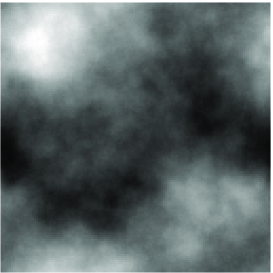
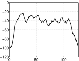
(a) True image

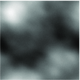
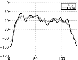
(b) Data

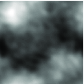
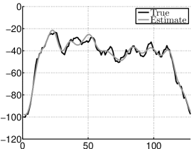
(c) Non-myopic

(d) Myopic

Fig. 1: The figure 1(a) represents a $128\times 128$ sample of the a priori law for the object with $\gamma_{0}=1$ and $\gamma_{1}=2$. Fig. 1(b) is the data computed with the PSF shown in Fig. 2. Figs. 1(c) and 1(d) are the estimates with non-myopic and the myopic estimate, respectively. Profiles correspond to the 68-th line.

These parameters provide the image shown in Fig. 1(a) : it is an image with smooth features similar to a cloud. Pixels have numerical values between $-100$ and $150$, and the profile line 68 shows fluctuations around a value of $-40$.

The a priori law for the hyperparameters are set to the non-informative Jeffreys’ law by fixing the $(\alpha_{i},\beta_{i})$ to $(0,+\infty)$, as explained in Sec. 3.C. In addition, the PSF is obtained in the Fourier space by discretization of a normalized Gaussian shape

$$\overset{\kern-3.30002pt~{}_{\circ}}{h}(\nu_{\alpha},\nu_{\beta})=\exp\bigg{(}-2\pi^{2}\Big{(}\nu_{\alpha}^{2}(w_{\alpha}\cos^{2}\varphi+w_{\beta}\sin^{2}\varphi)\\ +\nu_{\beta}^{2}(w_{\alpha}\sin^{2}\varphi+w_{\beta}\cos^{2}\varphi)\\ +2\nu_{\alpha}\nu_{\beta}\sin\varphi\cos\varphi\left(w_{\alpha}-w_{\beta}\right)\Big{)}\bigg{)}$$ (45)

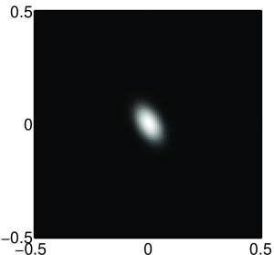
Fig. 2: PSF with $w_{\alpha}=20$, $w_{\beta}=7$ and $\varphi=\pi/3$. The x-axis and y-axis are reduced frequency.

with frequencies $(\nu_{\alpha},\nu_{\beta})\in\left[-0.5;0.5\right]^{2}$. This low-pass filter, illustrated in Fig. 2, is controlled by three parameters:

• two width parameters $w_{\alpha}$ and $w_{\beta}$ set to 20 and 7, respectively. Their a priori laws are uniform: $p(w_{\alpha})={\mathcal{U}}_{[19~{}21]}(w_{\alpha})$ and $p(w_{\beta})={\mathcal{U}}_{[6~{}8]}(w_{\alpha})$ corresponding to an uncertainty of about 5% and 15% around the nominal value (see Sec 3.D).

• a rotation parameter $\varphi$ set to $\pi/3$. The a priori law is also uniform $p(\varphi)={\mathcal{U}}_{[\pi/4~{}\pi/2]}(\varphi)$ corresponding to 50% uncertainty.

Then, the convolution is computed in the Fourier space and the data are obtained by adding a white Gaussian noise with precision $\gamma_{\epsilon}=0.5$. Data are shown Fig. 1(b): they are naturally smoother than the true image and the small fluctuations are less visible and corrupted by the noise. The empirical mean level of the image is correctly observed (the null frequency coefficient of ${\mathb{H}}_{\mathb{w}}$ is $\overset{\kern-3.30002pt~{}_{\circ}}{h}_{0}=1$) so the parameter $\gamma_{0}$ is considered as a nuisance parameter. Consequently it is integrated out under a Dirac (see Sec. 4). This is equivalent to fix its value to 0 in the algorithm Fig. 9, line 4.

Finally, the method is evaluated on two different situations.

1. The unsupervised and non-myopic case: the parameters ${\mathb{w}}$ are known. Consequently, there is no Metropolis-Hastings step (Sec. 5.C): lines 9 to 16 are ignored in the algorithm of Fig. 9 and ${\mathb{w}}$ is set to its true value. To obtain sufficient law exploration, the algorithm is run until the difference between two successive empirical means is less than $10^{-3}$. In this case, 921 samples are necessary and they are computed in approximately 12 seconds on a processor at 2.66 GHz with Matlab,

2. The unsupervised and myopic case: all the parameters are estimated. To obtain sufficient law exploration, the algorithm is run until the difference between two successive empirical means is less than $5\times 10^{-5}$. In this case, 18 715 samples are needed and they are computed in approximately 7 minutes.

Remark 2

—  The algorithm has also been run for up to 1 000 000 samples, in both cases, without perceptible qualitative changes.

6.B Estimation results

6.B.1 Images

The two results for the image are given Figs. 1(c) and 1(d) for the non-myopic and the myopic cases, respectively.

The effect of deconvolution is notable on the image, as well as on the shown profile. The object is correctly positioned, the orders of magnitude are respected and the mean level is correctly reconstructed. The image is restored, more details are visible and the profiles are closer matching to the true image than data. More precisely, the pixels 20-25 of the 68-th line in Fig. 1 show the restoration of the original dynamic whereas it is not visible in the data. Between pixels 70 and 110, fluctuations not visible in data are also correctly restored.

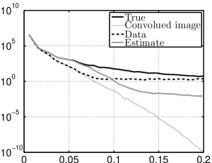
(a) Non-Myopic

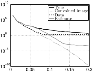
(b) Myopic

Fig. 3: Circular average of the empirical power spectral density of the image, the convolued image, the data (convolued image corrupted by noise) and the estimates, in radial frequency with y-axis in logarithmic scale. The x-axis is the radial frequency.

In order to visualize and study the spectral contents of the images, circular average of empirical power spectral density is considered and called “spectrum” hereafter. The subjacent spectral variable is a radial frequency $f$ such as $f^{2}=\nu_{\alpha}^{2}+\nu_{\beta}^{2}$. The spectrum of the true object, data and restored object are shown Figs. 3(a) and 3(b) in non-myopic and myopic cases, respectively. It is clear that the spectrum of the true image is correctly retrieved, in both cases, up to the radial frequency $f\approx 0.075$. Above this frequency, noise is clearly dominant and information about the image is almost lost. In other words, the method produces correct spectral equalization in the properly observed frequency band. The result is expected from a Wiener-Hunt method but the achievement is the joint estimation of hyperparameter and instrument parameters in addition to the correct spectral equalization.

Concerning a comparison between non-myopic and myopic cases, there is no visual differences. The spectrum Figs. 3(a) and 3(b) in non-myopic and myopic cases respectively are visually indistinguishable. This is also the case when comparing Figs. 1(c) and 1(d) and especially 68-th line. From a more precise quantitative evaluation, a slight difference is observed and detailed below.

In order to quantify performances, a normalized euclidean distance

$$e=\|{\mathb{x}}-{\mathb{x}}^{*}\|/\|{\mathb{x}}^{*}\|$$ (46)

between an image ${\mathb{x}}$ and the true image ${\mathb{x}}^{*}$ is considered. It is computed between true image and estimate images as well as between true image and data. Results are reported in Tab. 1 and confirm that the deconvolution is effective with an error of approximately 6 % in myopic case compared to 11 % with data. Both non-myopic and myopic deconvolution reduce error by a factor 1.7 with respect to the observed data.

Regarding a comparison between non-myopic and myopic case, the errors are almost the same, with a slightly lower value for the non-myopic case, as expected. This difference is coherent with the intuition: more information are injected in the non-myopic case through the true PSF parameters values.

6.B.2 Hyperparameters and instrument parameters

Concerning the other parameters, their estimates are close to the true values and are reported in Tab. 2. The $\gamma_{\epsilon}$ estimate is very close to the true value with $\widehat{\gamma_{\epsilon}}=0.49$ instead of 0.5 in the two cases. The error for the PSF parameters are 0.35%, 2.7% and 1.9% for $w_{\alpha}$, $w_{\beta}$ and $\varphi$, respectively. The value of $\gamma_{1}$ is underestimated in the two cases with approximately 1.7 instead of 2. All the true values fall in the $\hat{\mu}\pm 3\hat{\sigma}$ interval.

In order to deepen the numerical study, the paper evaluates the capability of the method to accurately select the best values for hyperparameters and instrument parameters. To this end, we compute the estimation error Eq. (46) for a set of “exhaustive” values of the parameters $[\gamma_{\epsilon},\gamma_{1},w_{\alpha},w_{\beta},\varphi]$. The protocol is the following: 1) choose a new value for a parameter ($\gamma_{\epsilon}$ for example) and fix the other parameters to the value provided by our algorithm, 2) compute the Wiener-Hunt solution (Sec. 5.A) and 3) compute the error index.

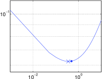
(a) $\gamma_{\epsilon}$

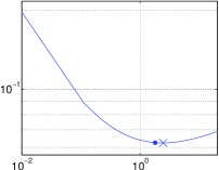
(b) $\gamma_{1}$

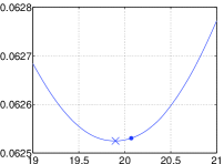
(c) $w_{\alpha}$

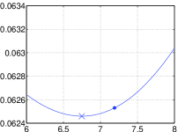
(d) $w_{\beta}$

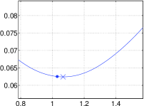
(e) $\varphi$

Fig. 4: Computation of the best parameters in the sense $e$ Eq. (46). The symbol ’$\times$’ is the minimum and the symbol ’.’ is the estimated value by our approach. The y-axis of $\gamma_{\epsilon}$ and $\gamma_{1}$ are in logarithmic scale.

Results are reported in Fig. 4. In each case, smooth variation of error is observed when varying hyperparameters and instrument parameters and an unique optimum is visible. By this way, one can find the value of the parameters that provide the best Wiener-Hunt solution when the true image ${\mathb{x}}^{\star}$ is known. It is reported on Tab. 1 and shows almost imperceptible improvement: optimization of the parameters (based on the true image ${\mathb{x}}^{\star}$) allow negligible improvement (smaller than 0.02 % as reported in Tab. 1).

So, the main conclusion is that, the unsupervised and myopic proposed approach is a relevant tool in order to tune parameters: it works (without the knowledge of the true image), as well as an optimal approach (based on the knowledge of the true image).

6.C A posteriori law characteristics

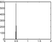
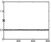
(a) $\gamma_{\epsilon}$ for non-myopic case

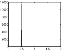
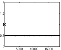
(b) $\gamma_{\epsilon}$ for myopic case

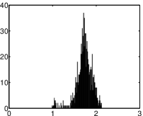
(c) $\gamma_{1}$ for non-myopic case

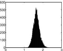
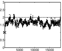
(d) $\gamma_{1}$ for myopic case

Fig. 5: Histograms and chains for the non-myopic case in Figs. 5(a)-5(c) and the myopic case in Figs. 5(b)-5(d) for $\gamma_{\epsilon}$ and $\gamma_{1}$, respectively. The symbol $\times$ localizes the initial value and the dashed line corresponds to the true value. The x-axis are iteration’s index for the chains and parameter value for the histograms.

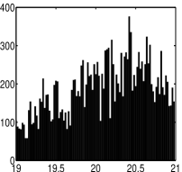
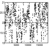
(a) $w_{\alpha}$

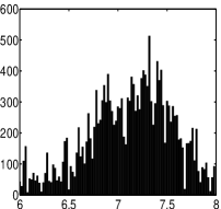
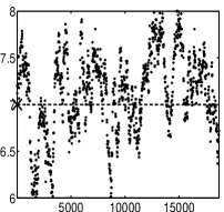
(b) $w_{\beta}$

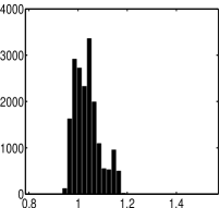
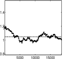
(c) $\varphi$

Fig. 6: Histogram and chain for the PSF parameters $w_{\alpha}$ in Fig. 6(a), $w_{\beta}$ in Fig. 6(b) and $\varphi$ in Fig. 6(c). The symbol $\times$ localizes the initial value and the dashed line corresponds to the true value. The x-axis for the histograms and the y-axis of the chain are limits of a priori law.

This section describes the a posteriori law using histograms, means and variances of the parameters. The sample histograms, Figs. 5 and 6, provide an approximation of the marginal posterior law for each parameter. Tabs. 1 and 2 report the variance for the image and law parameters respectively and thus allow to quantify the uncertainty.

6.C.1 Hyperparameter characteristics

The histograms for $\gamma_{\epsilon}$ and $\gamma_{1}$, Fig. 5, are concentrated around a mean value in both non-myopic and myopic cases. The variance for $\gamma_{\epsilon}$ is lower than the one for $\gamma_{1}$ and it can be explained as follows.

The observed data are directly impacted by noise (present at the system output) whereas they are indirectly impacted by the object (present at the system input). The convolution system damages the object and not the noise: as a consequence, the parameter $\gamma_{\epsilon}$ (that drives noise law) is more reliably estimated than $\gamma_{1}$ (that drives object law).

A second observation is the smaller variance for $\gamma_{1}$ in the non-myopic case Fig. 5(c) than in the myopic case Fig. 5(d). It is the consequence of the addition of information in the non-myopic case w.r.t. the myopic one, through the value of the PSF parameters. In the myopic case, the estimates are founded on the knowledge of an interval for the values of the instrument parameters, whereas in the non-myopic case, the estimates are founded on the true values for the instrument parameters.

6.C.2 PSF parameter characteristics

Fig. 6 gives histograms for the three PSF parameters and their appearances are quite different from the one for hyperparameters. The histograms for $w_{\alpha}$ and $w_{\beta}$, Figs. 6(a) and 6(b) are not as concentrated as the one of Fig. 5 for hyperparameters. Their variances are quite large with regards to the interval of the prior law. On the contrary, the histogram for the parameter $\varphi$, Fig. 6(c), has the smallest variance. It is analyzed as a consequence of a larger sensitivity of the data w.r.t. the parameter $\varphi$ than w.r.t. the parameters $w_{\alpha}$ and $w_{\beta}$. In an equivalent manner, the observed data are more informative about the parameter $\varphi$ than about the parameters $w_{\alpha}$ and $w_{\beta}$.

6.C.3 Mark of the myopic ambiguity

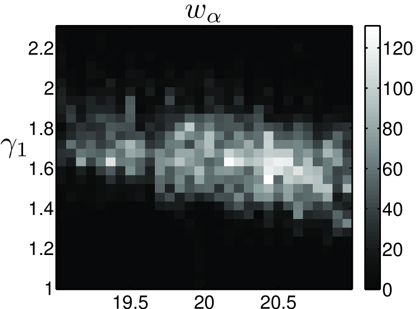
(a) $(\gamma_{1},w_{\alpha})$

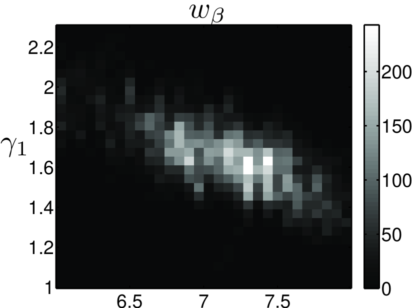
(b) $(\gamma_{1},w_{\beta})$

Fig. 7: Joint histograms for the couple $(\gamma_{1},w_{\alpha})$ and $(\gamma_{1},w_{\beta})$ in Figs. 7(a) and 7(b) respectively. The x-axis and y-axis are the parameter value.

Finally, a correlation between parameters $(\gamma_{1},w_{\alpha})$ and $(\gamma_{1},w_{\beta})$ is visible on their joint histograms Fig. 7. It can be interpreted as a consequence of the ambiguity in the primitive myopic deconvolution problem, in the following manner: the parameters $\gamma_{1}$ and ${\mathb{w}}$ both participate in the interpretation of the spectral content of data, $\gamma_{1}$ as a scale factor and ${\mathb{w}}$ as a shape factor. An increase of $w_{\alpha}$ or $w_{\beta}$ results in a decrease of the cutoff frequency of the observation system. In order to explain the spectral content of a given data set, the spectrum of the original image must contain more high frequencies, i.e., a smaller $\gamma_{1}$. This is also observed on the histogram illustrated Fig. 7(a).

6.D MCMC algorithm characteristics

Globally, the chains of Figs. 5 and 6, have a Markov feature (correlated) and explore the parameter space. They have a burn-in period followed by a stationary state. This characteristic has always been observed regardless the initialization. For fixed experimental conditions, the stationary state of multiple runs was always around the same value. Considering different initializations, the only visible change is on the length of the burn-in period.

More precisely, the chain of $\gamma_{\epsilon}$ is concentrated in a small interval, the burn-in period is very short (less than 10 samples) and its evolution seems independent of the other parameters. The chain of $\gamma_{1}$ has a larger exploration, the burn-in period is longer (approximately 200 samples) and the histogram is larger. This is in accordance with the analysis of Section 6.C.1.

About the PSF parameters, the behaviour is different for $(w_{\alpha},w_{\beta})$ and $\varphi$. The chain of the two width parameters has a very good exploration with quasi-instantaneous burn-in period. Conversely, the chain of $\varphi$ is more concentrated and its burn-in period is approximately 4 000 samples. This is also in accordance with previous analysis (Section 6.C.2).

Acceptation rates in the Metropolis-Hastings algorithm are reported in Tab. 3: they are quite small, especially for the rotation parameter. This is due to the structure of the implemented algorithm: an independant Metropolis-Hastings algorithm with the prior law as a proposition law. The main advantage of this choice is its simplicity but as a counterpart, a high rejection rate is observed due to a large a priori interval for the angle parameter. A future work will be devoted to the design of more accurate proposition law.

6.E Robustness of prior image model

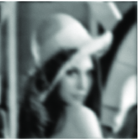
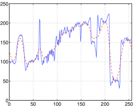
(a) Data

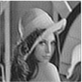
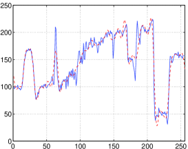
(b) Estimated image

Fig. 8: Observed image Fig. 8(a) and restored image Fig. 8(b). Profiles correspond to the 68-th line. The solid line is the true profile. Dashed line correspond to data in Fig. 8(a) and estimated profiles in Fig. 8(b).

Fig. 8 illustrates the proposed method on a more realistic image with heterogeneous spatial structures. The original is the Lena image and the data has been obtained with the same Gaussian PSF and also corruption by white Gaussian noise. The Fig. 8(b) shows that the restored image is closer to the true one than the data. Smaller structures are visible and edges are sharper, for example around pixel $200$. The estimated parameters are $\widehat{\gamma_{\epsilon}}=1.98$ while the true value is $\gamma_{\epsilon}^{\star}=2$. Concerning the PSF parameters, the results are $\widehat{w_{\alpha}}=19.3$, $\widehat{w_{\beta}}=7.5$ and $\widehat{\varphi}=1.15$ while the true values are respectively $w_{\alpha}^{\star}=20$, $w_{\beta}^{\star}=7$ and $\varphi^{\star}=1.05$ as in the previous section. Here again, the estimated PSF parameters are close to the true values giving a first assessment of the capability of the method in a more realistic context.

7 Conclusion and perspectives

This paper presents a new global and coherent method for myopic and unsupervised deconvolution of relatively smooth images. It is built within a Bayesian framework and a proper extended a posteriori law for the PSF parameters, the hyperparameters and the image. The estimate, defined as the posterior mean, is computed by means of an MCMC algorithm in less than a few minutes.

Numerical assessment testifies that the parameters of the PSF and the parameters of the prior laws are precisely estimated. In addition, results also demonstrate that the myopic and unsupervised deconvolved image is closer to the true image than the data and show true restored high-frequencies as well as spatial details.

The paper focuses on linear invariant model often encountered in astronomy, medical imaging, nondestructive testing and especially in optical problems. Non-invariant linear models can also be considered in order to address other applications such as spectrometry [4] or fluorescence microscopy [13]. The loss of invariance property precludes entirely Fourier-based computations but the methodology remains valid and practicable. In particular, it is possible to draw samples of the image by means of an optimization algorithm [38].

Gaussian law, related to $\mbox{L}_{2}$ penalization, is known for possible excessive sharp edges penalization in the restored object. The use of convex $\mbox{L}_{2}-\mbox{L}_{1}$ penalization [39, 40, 41] or non convex $\mbox{L}_{2}-\mbox{L}_{0}$ penalization [42] can overcome this limitation. In these cases a difficulty occurs in the development of myopic and unsupervised deconvolution: the partition function of the prior law for the image is in intricate or even unknown dependency w.r.t. the parameters [1, 43, 7]. However a recent paper [41] overcome the difficulty resulting in an efficient unsupervised deconvolution and we plan to extend this work for the myopic case.

Regarding noise, Gaussian likelihood limits robustness to outliers or aberrant data and it is possible to appeal to robust law such as Huber penalization in order to bypass the limitation. Nevertheless, the partition function for the noise law is again difficult or impossible to manage and it is possible to resort to the idea proposed in [41] to overcome the difficulty.

Finally, estimation of parameters of correlation matrix (cutoff frequency, attenuation coefficients,…) is possible within the same methodological framework. This could be achieved for the correlation matrix of the object or the noise. As for the PSF parameters, the approach could rely on an extended a posteriori law, including the new parameters and a Metropolis-Hastings sampler.

8 Acknowledgment

The authors would like to thank Professor Alain Abergel in IAS laboratory at Université Paris-Sud 11, France, for fruitful discussions and constructive suggestions. The authors are also grateful to Cornelia Vacar, IMS laboratory, for carefully reading the paper.

Appendix A Law in Fourier space

For a Gaussian vector ${\mathb{x}}\sim\mathcal{N}({\boldsymbol{\mu}},{\boldsymbol{\Sigma}})$, the law for $\overset{\kern-3.30002pt~{}_{\circ}}{{\mathb{x}}}={\mathb{F}}{\mathb{x}}$ (the fft of ${\mathb{x}}$) is also Gaussian whose first two moments are the following:

• The mean is

  $$\overset{\kern-3.30002pt~{}_{\circ}}{{\boldsymbol{\mu}}}=\mathds{E}[\overset{\kern-3.30002pt~{}_{\circ}}{{\mathb{x}}}]={\mathb{F}}\mathds{E}[\overset{\kern-3.30002pt~{}_{\circ}}{{\mathb{x}}}]={\mathb{F}}{\boldsymbol{\mu}}.$$ (47)

• The covariance matrix is

  $$\overset{\kern-3.30002pt~{}_{\circ}}{{\boldsymbol{\Sigma}}}=\mathds{E}[(\overset{\kern-3.30002pt~{}_{\circ}}{{\mathb{x}}}-\overset{\kern-3.30002pt~{}_{\circ}}{{\boldsymbol{\mu}}})(\overset{\kern-3.30002pt~{}_{\circ}}{{\mathb{x}}}-\overset{\kern-3.30002pt~{}_{\circ}}{{\boldsymbol{\mu}}})^{\dagger}]={\mathb{F}}{\boldsymbol{\Sigma}}{\mathb{F}}^{\dagger}.$$ (48)

Moreover, if the covariance matrix ${\boldsymbol{\Sigma}}$ is circulant it writes

$$\overset{\kern-3.30002pt~{}_{\circ}}{{\boldsymbol{\Sigma}}}={\mathb{F}}{\boldsymbol{\Sigma}}{\mathb{F}}^{\dagger}={\boldsymbol{\Lambda}}_{\boldsymbol{\Sigma}}.$$ (49)

i.e., the covariance matrix $\overset{\kern-3.30002pt~{}_{\circ}}{{\boldsymbol{\Sigma}}}$ is diagonal.

Appendix B The Gamma probability density

B.A Definition

The Gamma pdf for $\gamma>0$, with given parameter $\alpha>0$ and $\beta>0$, is written

$$\mathcal{G}(\gamma|\alpha,\beta)=\frac{1}{\beta^{\alpha}\Gamma(\alpha)}\gamma^{\alpha-1}\exp\left(-\gamma/\beta\right).$$ (50)

Tab. 4 gives three limit cases for $(\alpha,\beta)$. The following properties hold:

• The mean is $\mathds{E}_{\mathcal{G}}[\gamma]=\alpha\beta$

• The variance is $\mathds{V}_{\mathcal{G}}[\gamma]=\alpha\beta^{2}$

• The maximiser is $\beta(\alpha-1)$ if and only if $\alpha>1$

B.B Marginalisation

First consider a $N$ dimensional zero-mean Gaussian vector with a given precision matrix $\gamma{\boldsymbol{\Gamma}}$ with $\gamma>0$. The pdf reads

$$p({\mathb{x}}|\gamma)=(2\pi)^{-N/2}\gamma^{N/2}\det[{\boldsymbol{\Gamma}}]^{1/2}\,\exp\left[-\gamma{\mathb{x}}^{t}{\boldsymbol{\Gamma}}{\mathb{x}}\,/2\right]\,.$$ (51)

So consider the conjugate pdf for $\gamma$ as a Gamma law with parameter $(\alpha,\beta)$ (see previous Annex). The joint law for $({\mathb{x}},\gamma)$ is the product of the pdf given by Eq. (50) and Eq. (51): $p({\mathb{x}},\gamma)=p({\mathb{x}}|\gamma)p(\gamma)$. The marginalization of the joint law is known [44]:

$$\begin{split}p({\mathb{x}})&=\int_{\mathds{R}_{+}}p({\mathb{x}}|\gamma)p(\gamma)\,{\mathrm{d}}\gamma\\ &=\frac{\beta^{N/2}\det[{\boldsymbol{\Gamma}}]^{1/2}\Gamma\left(\alpha+N/2\right)}{(2\pi)^{N/2}\Gamma(\alpha)}\left(1+\frac{\beta{\mathb{x}}^{t}{\boldsymbol{\Gamma}}{\mathb{x}}}{2}\right)^{-\alpha-N/2}\end{split}$$ (52)

which is a $N$ dimensional t-Student law of $2\alpha$ degrees of freedom with a $\beta\Gamma$ precision matrix. Finally, the conditional law reads:

$$p(\gamma|{\mathb{x}})=\frac{(2\pi)^{-N/2}\det[{\boldsymbol{\Gamma}}]^{1/2}}{\beta^{\alpha}\Gamma(\alpha)}~{}~{}\gamma^{\alpha+N/2-1}\,\exp\left[-\gamma\left({\mathb{x}}^{t}{\boldsymbol{\Gamma}}{\mathb{x}}\,/2+1/\beta\right)\right]\,.$$ (53)

Thanks to conjugacy, it is also a Gamma pdf with parameters $\bar{\alpha}\,,\,\bar{\beta}$ given by $\bar{\alpha}=\alpha+N/2$ and $\bar{\beta}^{-1}=\beta^{-1}+2/({\mathb{x}}^{t}{\boldsymbol{\Gamma}}{\mathb{x}})$.

Appendix C The Metropolis-Hastings algorithm

The Metropolis-Hastings algorithm provides samples of a target law $f({\mathb{w}})$ that cannot be directly sampled but can be evaluated, at least up to a multiplicative constant. Using the so called “instrument law” $q\left({\mathb{w}}_{\mathrm{p}}|{\mathb{w}}^{(t)}\right)$, samples of the target law are obtained by the following iterations.

1. Sample a proposition ${\mathb{w}}_{\mathrm{p}}\sim q\left({\mathb{w}}_{\mathrm{p}}|{\mathb{w}}^{(t)}\right)$.

2. Compute the probability

   $$\rho=\min\left\{\frac{f\left({\mathb{w}}_{\mathrm{p}}\right)}{f\left({\mathb{w}}^{(t)}\right)}\frac{q\left({\mathb{w}}^{(t)}|{\mathb{w}}_{\mathrm{p}}\right)}{q\left({\mathb{w}}_{\mathrm{p}}|{\mathb{w}}^{(t)}\right)},1\right\}.$$ (54)

3. Take

   $${\mathb{w}}^{(t+1)}=\left\{\begin{array}[]{cl}{\mathb{w}}_{\mathrm{p}}&\text{with~{}}\rho\text{~{}probability~{}}\\ {\mathb{w}}^{(t)}&\text{with~{}}1-\rho\text{~{}probability~{}}.\end{array}\right.$$ (55)

At convergence, the samples follow the target law $f({\mathb{w}})$ [25, 36]. When $q\left({\mathb{w}}_{\mathrm{p}}|{\mathb{w}}^{(t)}\right)=q({\mathb{w}}_{\mathrm{p}})$ the algorithm is named independent Metropolis-Hastings. In addition, if the instrument law is uniform, the acceptance probability gets simpler in

$$\rho=\min\left\{\frac{f\left({\mathb{w}}_{\mathrm{p}}\right)}{f\left({\mathb{w}}^{(t)}\right)},1\right\}.$$ (56)

Table 1: Error $e$ (Eq. (46)) and averaged standard deviation $\hat{\sigma}$ of the posterior image law. The “Best” error has been obtained with the knowledge of the true image.

	Data	Non-myopic	Myopic	Best
Error ($e$)	11.092 %	6.241 %	6.253 %	6.235 %
$\hat{\sigma}$ of ${\mathb{x}}$ law	-	3.16	3.25	-

Table 2: Quantitative evaluation: true and estimated values of hyperparameters and PSF parameters.

		$\widehat{\gamma}_{\epsilon}\pm\hat{\sigma}$	$\widehat{\gamma}_{1}\pm\hat{\sigma}$	$\widehat{w}_{\alpha}\pm\hat{\sigma}$	$\widehat{w}_{\beta}\pm\hat{\sigma}$	$\widehat{\varphi}\pm\hat{\sigma}$
	True value	0.5	2	20	7	1.05 ($\pi/3$)
Non-myopic	Estimate	0.49 $\pm 0.0056$	1.78 $\pm 0.14$	-	-	-
	Error	2.0 %	11 %	-	-	-
Myopic	Estimate	0.49 $\pm 0.0056$	1.65 $\pm 0.15$	20.07 $\pm 0.53$	7.19 $\pm 0.38$	1.03 $\pm 0.04$
	Error	2.0 %	18 %	0.35 %	2.7 %	1.9 %

Table 3: Acceptation rate.

Parameter	$w_{\alpha}$	$w_{\beta}$	$\varphi$
Acceptation rate	14.50 %	9.44 %	2.14 %

Table 4: Specific laws obtained as limit of the Gamma pdf.

	$\alpha$	$\beta$
Jeffreys	0	$+\infty$
Uniform	1	$+\infty$
Dirac	-	0

1:Initialisation of $\left[\overset{\kern-3.30002pt~{}_{\circ}}{{\mathb{x}}}^{(0)},{\boldsymbol{\gamma}}^{(0)},{\mathb{w}}^{(0)},k=0\right]$

2:repeat% Sample of $\overset{\kern-3.30002pt~{}_{\circ}}{{\mathb{x}}}$

3:     ${\boldsymbol{\Sigma}}\leftarrow\gamma_{\epsilon}^{(k)}|{\boldsymbol{\Lambda}}_{{\mathb{H}}}|^{2}+\gamma_{0}^{(k)}|{\boldsymbol{\Lambda}}_{\mathds{1}}|^{2}+\gamma_{1}^{(k)}|{\boldsymbol{\Lambda}}_{{\mathb{D}}}|^{2}$

4:     ${\boldsymbol{\mu}}\leftarrow\gamma_{\epsilon}^{(k)}{\boldsymbol{\Sigma}}^{-1}{\boldsymbol{\Lambda}}_{{\mathb{H}}}^{*}~{}\overset{\kern-3.30002pt~{}_{\circ}}{{\mathb{y}}}$

5:     $\overset{\kern-3.30002pt~{}_{\circ}}{{\mathb{x}}}^{(k)}\leftarrow{\boldsymbol{\mu}}+{\boldsymbol{\Sigma}}^{-1/2}.*\mathtt{randn}$ % Sample of ${\boldsymbol{\gamma}}$

6:     $\gamma_{\epsilon}^{(k)}\leftarrow\mathtt{gamrnd}(\alpha_{\epsilon},\beta_{\epsilon})$

7:     $\gamma_{1}^{(k)}\leftarrow\mathtt{gamrnd}(\alpha_{1},\beta_{1})$

8:     $\gamma_{0}^{(k)}\leftarrow\mathtt{gamrnd}(\alpha_{0},\beta_{0})$ % Sample of ${\mathb{w}}$

9:     ${\mathb{w}}_{{\mathrm{p}}}\leftarrow\mathtt{rand}*({\mathb{a}}-{\mathb{b}})+{\mathb{a}}$

10:     $J\leftarrow\gamma_{\epsilon}\left(\|\overset{\kern-3.30002pt~{}_{\circ}}{{\mathb{y}}}-{\boldsymbol{\Lambda}}_{{\mathb{H}}}\,\overset{\kern-3.30002pt~{}_{\circ}}{{\mathb{x}}}\|^{2}-\|\overset{\kern-3.30002pt~{}_{\circ}}{{\mathb{y}}}-{\boldsymbol{\Lambda}}_{{\mathb{H}},{\mathb{w}}_{{\mathrm{p}}}}\,\overset{\kern-3.30002pt~{}_{\circ}}{{\mathb{x}}}\|^{2}\right)/2$

11:     if $\log(\mathtt{rand})<\min\{J,0\}$ then

12:     ${\mathb{w}}^{(k)}\leftarrow{\mathb{w}}_{{\mathrm{p}}}$

13:     ${\boldsymbol{\Lambda}}_{{\mathb{H}}}\leftarrow{\boldsymbol{\Lambda}}_{{\mathb{H}},{\mathb{w}}_{{\mathrm{p}}}}$

14:     else

15:     ${\mathb{w}}^{(k)}\leftarrow{\mathb{w}}^{(k-1)}$

16:     end if % Empirical mean

17:     $k\leftarrow k+1$

18:     $\overset{\kern-3.30002pt~{}_{\circ}}{\bar{\mathb{x}}}^{(k)}\leftarrow\sum_{i}\overset{\kern-3.30002pt~{}_{\circ}}{{\mathb{x}}}^{(i)}/k$

19:until $|\bar{\mathb{x}}^{(k)}-\bar{\mathb{x}}^{(k-1)}|/|\bar{\mathb{x}}^{(k)}|\leq\text{criterion}$

Fig. 9: Pseudo-code algorithm. $\mathtt{gamrnd,rand}$ and $\mathtt{randn}$ draw samples of gamma variable, uniform variable, and zero-mean unit-variance white complex Gaussian vector respectively.

References

- [1] J. Idier, ed., Bayesian Approach to Inverse Problems (ISTE Ltd and John Wiley & Sons Inc., London, 2008).
- [2] R. Molina, J. Mateos, and A. K. Katsaggelos, “Blind deconvolution using a variational approach to parameter, image, and blur estimation,” IEEE Trans. Image Processing 15, 3715–3727 (2006).
- [3] P. Campisi and K. Egiazarian, eds., Blind Image Deconvolution (CRC Press, 2007).
- [4] T. Rodet, F. Orieux, J.-F. Giovannelli, and A. Abergel, “Data inversion for over-resolved spectral imaging in astronomy,” IEEE J. of Selec. Topics in Signal Proc. 2, 802–811 (2008).
- [5] A. Tikhonov and V. Arsenin, Solutions of Ill-Posed Problems (Winston, Washington, dc, 1977).
- [6] S. Twomey, “On the numerical solution of Fredholm integral equations of the first kind by the inversion of the linear system produced by quadrature,” J. Assoc. Comp. Mach. 10, 97–101 (1962).
- [7] A. Jalobeanu, L. Blanc-Féraud, and J. Zerubia, “Hyperparameter estimation for satellite image restoration by a MCMC maximum likelihood method,” Pattern Recognition 35, 341–352 (2002).
- [8] J. A. O’Sullivan, “Roughness penalties on finite domains,” IEEE Trans. Image Processing 4, 1258–1268 (1995).
- [9] G. Demoment, “Image reconstruction and restoration: Overview of common estimation structure and problems,” IEEE Trans. Acoust. Speech, Signal Processing assp-37, 2024–2036 (1989).
- [10] P. Pankajakshani, B. Zhang, L. Blanc-Féraud, Z. Kam, J.-C. Olivo-Marin, and J. Zerubia, “Blind deconvolution for thin-layered confocal imaging,” Appl. Opt. 48, 4437–4448 (2009).
- [11] E. Thi baut and J.-M. Conan, “Strict a priori constraints for maximum likelihood blind deconvolution,” J. Opt. Soc. Am. A 12, 485–492 (1995).
- [12] N. Dobigeon, A. Hero, and J.-Y. Tourneret, “Hierarchical bayesian sparse image reconstruction with application to MRFM,” IEEE Trans. Image Processing (2009).
- [13] B. Zhang, J. Zerubia, and J.-C. Olivo-Marin, “Gaussian approximations of fluorescence microscope point-spread function models,” Appl. Opt. 46, 1819–1829 (2007).
- [14] L. Mugnier, T. Fusco, and J.-M. Conan, “MISTRAL: a myopic edge-preserving image restoration method, with application to astronomical adaptive-optics-corrected long-exposure images,” J. Opt. Soc. Amer. 21, 1841–1854 (2004).
- [15] E. Thiébaut, “MiRA: an effective imaging algorithm for optical interferometry,” in “proc. SPIE: Astronomical Telescopes and Instrumentation,” , vol. 7013 (2008), vol. 7013, pp. 70131–I.
- [16] T. Fusco, J.-P. V. ran, J.-M. Conan, and L. M. Mugnier, “Myopic deconvolution method for adaptive optics images of stellar fields,” Astron. Astrophys. Suppl. Ser. 134, 193 (1999).
- [17] J.-M. Conan, L. Mugnier, T. Fusco, V. Michau, and R. G., “Myopic deconvolution of adaptive optics images by use of object and point-spread function power spectra,” Applied Optics 37, 4614–4622 (1998).
- [18] A. C. Likas and N. P. Galatsanos, “A variational approach for Bayesian blind image deconvolution,” IEEE Trans. Image Processing 52, 2222–2233 (2004).
- [19] T. Bishop, R. Molina, and J. Hopgood, “Blind restoration of blurred photographs via AR modelling and MCMC,” in “Image Processing, 2008. ICIP 2008. 15th IEEE Int. Conference on,” (2008).
- [20] E. Y. Lam and J. W. Goodman, “Iterative statistical approach to blind image deconvolution,” J. Opt. Soc. Am. A 17, 1177–1184 (2000).
- [21] Z. Xu and E. Y. Lam, “Maximum a posteriori blind image deconvolution with Huber–Markov random-field regularization,” Opt. Lett. 34, 1453–1455 (2009).
- [22] M. Cannon, “Blind deconvolution of spatially invariant image blurs with phase,” IEEE Trans. Acoust. Speech, Signal Processing 24, 58–63 (1976).
- [23] A. Jalobeanu, L. Blanc-Feraud, and J. Zerubia, “Estimation of blur and noise parameters in remote sensing,” in “Proc. IEEE ICASSP,” , vol. 4 (2002), vol. 4, pp. 3580–3583.
- [24] F. Chen and J. Ma, “An empirical identification method of Gaussian blur parameter for image deblurring,” Signal Processing, IEEE Trans. on (2009).
- [25] C. P. Robert and G. Casella, Monte-Carlo Statistical Methods, Springer Texts in Statistics (Springer, New York, ny, 2000).
- [26] B. R. Hunt, “A matrix theory proof of the discrete convolution theorem,” IEEE Trans. Automat. Contr. AC-19, 285–288 (1971).
- [27] M. Calder and R. A. Davis, “Introduction to Whittle (1953) ‘The analysis of multiple stationary time series’,” Breakthroughs in Statistics 3, 141–148 (1997).
- [28] P. J. Brockwell and R. A. Davis, Time Series: Theory and Methods (Springer-Verlag, New York, 1991).
- [29] B. R. Hunt, “Deconvolution of linear systems by constrained regression and its relationship to the Wiener theory,” IEEE Trans. Automat. Contr. AC-17, 703–705 (1972).
- [30] K. Mardia, J. Kent, and J. Bibby, Multivariate Analysis (San Diego : Academic Press, 1992), chap. 2, pp. 36–43.
- [31] C. A. Bouman and K. D. Sauer, “A generalized Gaussian image model for edge-preserving map estimation,” IEEE Trans. Image Processing 2, 296–310 (1993).
- [32] D. MacKay, Information Theory, Inference, and Learning Algorithms (Cambridge University Press, 2003).
- [33] R. E. Kass and L. Wasserman, “The selection of prior distributions by formal rules,” J. Amer. Statist. Assoc. 91, 1343–1370 (1996).
- [34] E. T. Jaynes, Probability Theory: The Logic of Science (Cambridge University Press, 2003).
- [35] S. Lang, Real and functional analysis (Springer, 1993).
- [36] P. Brémaud, Markov Chains. Gibbs fields, Monte Carlo Simulation, and Queues, Texts in Applied Mathematics 31 (Spinger, New York, ny, 1999).
- [37] S. Geman and D. Geman, “Stochastic relaxation, Gibbs distributions, and the Bayesian restoration of images,” IEEE Trans. Pattern Anal. Mach. Intell. 6, 721–741 (1984).
- [38] F. Orieux, O. Féron, and J.-F. Giovannelli, “Stochastic sampling of large dimension non-stationnary gaussian field for image restoration,” Submitted to ICIP2010.
- [39] H. R. Künsch, “Robust priors for smoothing and image restoration,” Ann. Inst. Stat. Math. 46, 1–19 (1994).
- [40] P. Charbonnier, L. Blanc-Féraud, G. Aubert, and M. Barlaud, “Deterministic edge-preserving regularization in computed imaging,” IEEE Trans. Image Processing 6, 298–311 (1997).
- [41] J.-F. Giovannelli, “Unsupervised Bayesian convex deconvolution based on a field with an explicit partition function,” IEEE Trans. Image Processing 17, 16–26 (2008).
- [42] D. Geman and C. Yang, “Nonlinear image recovery with half-quadratic regularization,” IEEE Trans. Image Processing 4, 932–946 (1995).
- [43] X. Descombes, R. Morris, J. Zerubia, and M. Berthod, “Estimation of Markov random field prior parameters using Markov chain Monte Carlo maximum likelihood,” IEEE Trans. Image Processing 8, 954–963 (1999).
- [44] G. E. P. Box and G. C. Tiao, Bayesian inference in statistical analysis (Addison-Wesley publishing, 1972).