Crossing symmetric potential model of pion-nucleon scattering

Abstract

A crossing symmetric $\pi N$ scattering amplitude is constructed through a complete attachment of two external pions to the dressed nucleon propagator of an underlying $\pi N$ potential model. Our formulation automatically provides expressions also for the crossing symmetric and gauge invariant pion photoproduction and Compton scattering amplitudes. We show that our amplitudes are unitary if they coincide on-shell with the amplitudes obtained by attaching one pion to the dressed $\pi NN$ vertex of the same potential model.

1 Introduction

The $\pi N$ scattering amplitude $t$ is often described using the set of equations Morioka and Afnan (1982); Gross and Surya (1993); Pascalutsa and Tjon (2000)

$$t =fg\bar{f}+t_{b}, t_{b} =v+t_{b}G_{0}v,$$ (1a)

$$\bar{f} =\bar{f}_{0}+\bar{f}_{0}G_{0}t_{b}, f =f_{0}+t_{b}G_{0}f_{0},$$ (1b)

$$g =g_{0}+g_{0}\Sigma g, \Sigma =\bar{f}_{0}G_{0}f,$$ (1c)

where $f$ ($f_{0}$) is the dressed (bare) $N\rightarrow\pi N$ vertex, $\bar{f}$ ($\bar{f}_{0}$) is the dressed (bare) $\pi N\rightarrow N$ vertex, $g$ ($g_{0}$) is the dressed (bare) nucleon propagator, $G_{0}$ is the renormalized disconnected $\pi N$ propagator, and $t_{b}$ ($v$) is the ”non-pole” $\pi N$ t-matrix (potential) with the pole term $fg\bar{f}$ ($f_{0}g_{0}\bar{f}_{0}$) removed. Although these equations provide an exact description in full field theory, their main feature is that they allow one to preserve unitarity when making models for the potential $v$ and bare vertex $f_{0}$. However, like all potential models, these equations suffer from a lack of crossing symmetry, a property whose importance has been emphasized for more than 50 years Chew and Low (1956); McLeod (1984); Fernandez-Ramirez et al. (2008).

Similarly, the pion photoproduction amplitude $t^{\gamma}$ is often descsribed by a set of equations that essentially result from Eq. (1a) and Eq. (1b) by replacing the initial pion with a photon Nozawa et al. (1990); Surya and Gross (1996); Pascalutsa and Tjon (2004):

$$t^{\gamma} =fg\bar{f}^{\gamma}+t_{b}^{\gamma}, t_{b}^{\gamma} =v^{\gamma}+t_{b}G_{0}v^{\gamma},$$ (2a)

$$\bar{f}^{\gamma} =\bar{f}^{\gamma}_{0}+\bar{f}_{0}G_{0}t_{b}^{\gamma},$$ (2b)

where $\bar{f}^{\gamma}$ ($\bar{f}^{\gamma}_{0}$) is the dressed (bare) $\gamma N\rightarrow N$ vertex, and $t^{\gamma}_{b}$ ($v^{\gamma}$) is the pion photoproduction amplitude (Born term) with the pole term $fg\bar{f}^{\gamma}$ ($f_{0}g_{0}\bar{f}^{\gamma}_{0}$) removed. Once again the feature of these equations is that they respect unitarity. This time, however, these equations suffer not only from a lack of crossing symmetry, but also from the breaking of manifest gauge invariance (because the photon is not coupled to all places in the underlying field theory). We shall refer to Eqs. (1) and Eqs. (2) as the standard description.

In this paper we present new equations for $\pi N$ scattering, pion photoproduction, and Compton scattering, that are based on the potential model of Eqs. (1), but that preserve crossing symmetry and manifest gauge invariance. Our approach is based on the idea of coupling external pions and photons to all possible places in the dressed propagator $g$ of Eq. (1c), and is achieved using the gauging of equations method Kvinikhidze and Blankleider (1999a, b). Like the standard description, our approach is exact in full field theory; however, just opposite to the standard description, when models are made for the potential $v$ and bare vertex $f_{0}$, our approach preserves crossing symmetry and gauge invariance at the expense of unitarity. The lack of built-in unitarity is not surprising since our approach effectively sums the full perturbation series in a way that is different from the usual method of iterating a kernel. Nevertheless, we show that our amplitudes will satisfy unitarity whenever the crossing symmetric $\pi N$ amplitude coincides, on-shell, with the one obtained by attaching one pion to the dressed $\pi NN$ vertex $f$ of Eq. (1b).

2 Single-gauged amplitude

In Refs. Kvinikhidze and Blankleider (1999a, b) we introduced a technique for attaching an external photon to all possible places (vertices, propagators, potentials, etc.) within a strongly interacting system described by dynamical equations. The completeness of the attachment led to the gauge invariance of the resulting electromagnetic currents. Here we use the same technique to also attach first one external pion, and then in the next section, a second external pion, in order to achieve our goal of deriving a crossing symmetric $\pi N$ scattering amplitude.

We begin by applying our gauging technique to the $\pi N$ Green function $G$ generated by the non-pole potential $v$:

$$G=G_{0}+G_{0}vG.$$ (3)

Denoting by $G^{\mu}$ the 5-point function resulting from a complete attachment of an external pion to $G$, Eq. (3) is ”gauged” to obtain

$$G^{\mu}=G^{\mu}_{0}+G^{\mu}_{0}vG+G_{0}v^{\mu}G+G_{0}vG^{\mu}$$ (4)

which is easily solved to get

$$G^{\mu} =G\Lambda^{\mu}G, \Lambda^{\mu} =\Lambda_{0}^{\mu}+v^{\mu}$$ (5)

where $\Lambda_{0}^{\mu}\equiv G_{0}^{-1}G_{0}^{\mu}G_{0}^{-1}$ is a vertex function derived by attaching an external pion to the disconnected $\pi N$ propagator $G_{0}$. Note that $G_{0}=g_{\pi}g_{N}$ where $g_{\pi}$ is the pion propagator and $g_{N}$ is the renormalized nucleon propagator (in exact field theory $g_{N}=g/Z$ where $Z$ is the renormalization constant; however, in model calculations one usually takes $g_{N}$ to be the bare propagator with physical nucleon mass). As G-parity conservation forbids a three-pion vertex, $\Lambda_{0}^{\mu}=\Gamma_{N}^{\mu}g_{\pi}^{-1}$ where $\Gamma_{N}^{\mu}\equiv g_{N}^{-1}g_{N}^{\mu}g_{N}^{-1}$. Thus

$$\Lambda^{\mu}=\Gamma_{N}^{\mu}g_{\pi}^{-1}+v^{\mu}.$$ (6)

The gauged potential $v^{\mu}$ can be constructed phenomenologically, or derived by gauging a specific model for $v$. Similarly, the gauging of the dressed nucleon propagator $g$ of Eq. (1c), gives the 3-point function $g^{\mu}$:

$$g^{\mu} =g\Gamma^{\mu}g, \Gamma^{\mu} =\Gamma_{0}^{\mu}+\Sigma^{\mu}$$ (7)

where $\Gamma^{\mu}$ is the dressed $\pi NN$ vertex function, $\Gamma_{0}^{\mu}\equiv g_{0}^{-1}g_{0}^{\mu}g_{0}^{-1}$ is the bare vertex function, and $\Sigma^{\mu}$ is the gauged dressing. Gauging $\Sigma=\bar{f}_{0}Gf_{0}$ then leads to a simple intuitive expression for the $\pi NN$ dressed vertex function:

$$\Gamma^{\mu} =\Gamma_{0}^{\mu}+\bar{f}^{\mu}_{0}G_{0}f+\bar{f}G_{0}f^{\mu}_{0}+\bar{f}G_{0}^{\mu}f+\bar{f}G_{0}v^{\mu}G_{0}f,$$ (8)

which is illustrated in Fig. (1).

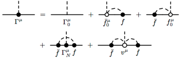
Figure 1: The dressed $\pi NN$ vertex function $\Gamma^{\mu}$ resulting from a complete pion attachment to the dressed nucleon propagator $g$ defined by Eq. (1c).

The main results of this section come from the gauging of the dressed $\pi NN$ vertrex $f$:

$$(G_{0}fg)^{\nu} =(Gf_{0}g)^{\nu}=G^{\nu}f_{0}g+Gf_{0}^{\nu}g+Gf_{0}g^{\nu}$$

$$=G\Lambda^{\nu}G_{0}fg+Gf_{0}^{\nu}g+G_{0}fg\Gamma^{\nu}g.$$ (9)

Cutting off the external legs immediately gives the amplitude $T^{\nu}\equiv G_{0}^{-1}(G_{0}fg)^{\nu}g^{-1}$:

$$T^{\nu}=(1+t_{b}G_{0})(\Lambda_{0}^{\nu}G_{0}f+v^{\mu}G_{0}f+f_{0}^{\nu})+fg\Gamma^{\nu}.$$ (10)

If superscript $\nu$ corresponds to an external photon, then $T^{\nu}\sqrt{Z}$ is the properly normalized manifestly gauge invariant pion photoproduction amplitude, originally derived in Ref. van Antwerpen and Afnan (1995) using a more involved approach. If superscript $\nu$ corresponds to an external pion, then $T^{\nu}\sqrt{Z}$ is a ”hybrid” $\pi N$ scattering amplitude where the initial state pion is due to gauging and the final state pion is due to the original standard description. In a similar way, vertex $\bar{f}$ can be gauged to obtain the hybrid amplitude $\bar{T}^{\mu}$ where the final state pion is due to gauging. One can express these amplitudes in a ”pole plus non-pole” form analogous to Eq. (1a):

$$T^{\nu} =fg\Gamma^{\nu}+T_{b}^{\nu}, T^{\nu}_{b} =(1+t_{b}G_{0})V^{\nu}, V^{\nu} =f_{0}^{\nu}+\Lambda^{\nu}G_{0}f,$$ (11a)

$$\bar{T}^{\mu} =\Gamma^{\mu}g\bar{f}+\bar{T}_{b}^{\mu}, \bar{T}^{\mu}_{b} =\bar{V}^{\mu}(1+G_{0}t_{b}), \bar{V}^{\mu} =\bar{f}_{0}^{\mu}+\bar{f}G_{0}\Lambda^{\mu}.$$ (11b)

It follows that amplitudes $T_{b}^{\nu}$ and $\bar{T}_{b}^{\mu}$ satisfy non-standard Bethe-Salpeter equations

$$T_{b}^{\nu} =V^{\nu}+vG_{0}T_{b}^{\nu}, \bar{T}_{b}^{\mu} =\bar{V}^{\mu}+\bar{T}_{b}^{\mu}G_{0}v$$ (12)

where the kernel and inhomogeneous terms involve $\pi N$ potentials of different origin. The amplitudes are clearly not crossing symmetric.

We can now express Eq. (8) in the following two ways analogous to Eq. (1b):

$$\Gamma^{\nu} =\bar{F}_{0}^{\nu}+\bar{f}G_{0}V^{\nu}, \bar{F}_{0}^{\nu} =\Gamma_{0}^{\nu}+\bar{f}^{\nu}_{0}G_{0}f,$$ (13a)

$$\Gamma^{\mu} =F_{0}^{\mu}+\bar{V}^{\mu}G_{0}f, F_{0}^{\mu} =\Gamma_{0}^{\mu}+\bar{f}G_{0}f^{\mu}_{0},$$ (13b)

where Eq. (13a) and Eq. (13b) are to be used to describe pion (or photon) absorption and creation vertices, respectively. In exact field theory, $\Gamma^{\mu}$ can be identified with function $f/\sqrt{Z}$ of the standard description. Eqs. (13) then imply the following identities (in exact field theory) relating the standard description quantities $f_{0}$ and $v$ (typically the model inputs) to their gauged counterparts:

$$f_{0}/\sqrt{Z} =F_{0}^{\mu}, v/\sqrt{Z} =\bar{V}^{\mu}; \bar{f}_{0}/\sqrt{Z} =\bar{F}_{0}^{\nu}, v/\sqrt{Z} =V^{\nu}.$$ (14)

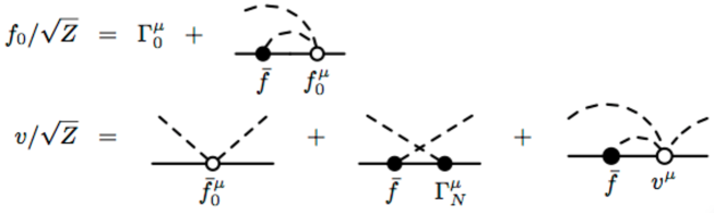
Figure 2: In exact field theory, relations connecting the bare $\pi NN$ vertex $f_{0}$ and ”non-pole” $\pi N$ potential $v$ of the standard description, Eqs. (1), to the corresponding gauged quantities $f_{0}^{\mu}$ and $v^{\mu}$ of the single-gauged description - see the first two of Eqs. (14).

The first two of Eqs. (14) are illustrated in Fig. 2.

2.1 Unitarity

For ease of presentation, we discuss unitarity within the framework of time ordered perturbation theory for which

$$G_{0}(E^{+})-G_{0}(E^{-})=-2\pi i\delta(E-H_{0})$$ (15)

where $H_{0}$ is the free Hamiltonian and $E^{\pm}=E\pm i\epsilon$. We consider only 2-body unitarity and thus restrict the discussion to energies $E$ below the two-pion threshold. In this energy region the potential $v$ and bare vertex $f_{0}$ are real, and the standard description of Eqs. (1) will therefore satisfy the following unitarity relations:

$$t-t^{\dagger} =t^{\dagger}\!\delta\,t, t_{b}-t_{b}^{\dagger} =t_{b}^{\dagger}\!\delta\,t_{b},$$ (16a)

$$f-f^{\dagger} =t_{b}^{\dagger}\delta f, \bar{f}-\bar{f}^{\dagger} =\bar{f}^{\dagger}\delta t_{b},$$ (16b)

$$g-g^{\dagger} =g^{\dagger}\,(\Sigma-\Sigma^{\dagger})\,g, \Sigma-\Sigma^{\dagger} =\bar{f}{\,}^{\dagger}\delta\,f,$$ (16c)

$$G-G^{\dagger} =(1+G_{0}^{\dagger}\,t_{b}^{\dagger})\,\delta\,(1+t_{b}G_{0}),$$ (16d)

where $\delta$ is shorthand for $-2\pi i\delta(E-H_{0})$ and where identical quantities with and without a dagger represent the same functions of $E^{-}$ and $E^{+}$, respectively (i.e., a dagger does not mean Hermitean conjugate, but rather, $T\equiv T(E^{+})$ and $T^{\dagger}\equiv T(E^{-})$). Applying these relations to Eqs. (11) and Eqs. (13) one obtains the analogous unitarity relations for the hybrid amplitudes:

$$T^{\nu}-T^{\nu}{}^{\dagger} =t^{\dagger}\!\delta\,T^{\nu}, T^{\nu}_{b}-T_{b}^{\nu}{}^{\dagger} =t_{b}^{\dagger}\!\delta\,T^{\nu}_{b},$$ (17a)

$$\bar{T}^{\mu}-\bar{T}^{\mu}{}^{\dagger} =\bar{T}^{\mu}{}^{\dagger}\!\delta\,t, \bar{T}^{\mu}_{b}-\bar{T}_{b}^{\mu}{}^{\dagger} =\bar{T}_{b}^{\mu}{}^{\dagger}\!\delta\,t_{b},$$ (17b)

$$\Gamma^{\mu}-\Gamma^{\mu}{}^{\dagger} =\bar{T}_{b}^{\mu}{}^{\dagger}\delta f, \Gamma^{\nu}-\Gamma^{\nu}{}^{\dagger} =\bar{f}^{\dagger}\delta T_{b}^{\nu}.$$ (17c)

In the case of gauging with photons, Eq. (17a) provides just the usual statement of Watson’s theorem for the gauge invariant pion photoproduction amplitude $T^{\nu}$. However, in the case of gauging with pions, Eq. (17a) differs from the usual statement of unitarity for the hybrid amplitude in that a $T^{\nu}{}^{\dagger}$ has been replaced with a $t^{\dagger}$ from the standard description. Thus the only way for a hybrid $\pi N$ amplitude $T^{\nu}$ to be unitary is for it to coincide, on-shell, with the standard amplitude $t$.

3 Double-gauged amplitude

To obtain a crossing symmetric $\pi N$ scattering amplitude, we attach two external pions to the dressed nucleon propagator $g$; that is, we first gauge $g$ to obtain $g^{\mu}$ as in Eq. (7), and then gauge Eq. (7) to obtain $g^{\mu\nu}$ with indices $\nu$ and $\mu$ denoting the initial- and final-state pion, respectively. Thus

$$g^{\mu\nu} =gT^{\mu\nu}g, T^{\mu\nu} =\Gamma^{\mu}g\Gamma^{\nu}+\Gamma^{\nu}g\Gamma^{\mu}+\Gamma_{0}^{\mu\nu}+\Sigma^{\mu\nu}$$ (18)

where $ZT^{\mu\nu}$ is the properly normalized crossing symmetric $\pi N$ amplitude. In Eq. (18)

$$\Gamma_{0}^{\mu\nu} =\left(g_{0}^{-1}g_{0}^{\mu}g_{0}^{-1}\right)^{\nu}=g_{0}^{-1}g_{0}^{\mu\nu}g_{0}^{-1}-\Gamma_{0}^{\mu}g_{0}\Gamma_{0}^{\nu}-\Gamma_{0}^{\nu}g_{0}\Gamma_{0}^{\mu},$$ (19a)

$$\Sigma^{\mu\nu} =\bar{f}_{0}^{\mu\nu}G_{0}f+\bar{f}G_{0}f_{0}^{\mu\nu}+\bar{f}G_{0}\Lambda^{\mu\nu}G_{0}f+A^{\mu\nu}+A^{\nu\mu}$$ (19b)

where

$$\Lambda^{\mu\nu} =\Gamma_{N}^{\mu\nu}g_{\pi}^{-1}+v^{\mu\nu},$$ (20a)

$$A^{\mu\nu} =\bar{V}^{\mu}GV^{\nu}=\bar{V}^{\mu}G_{0}T_{b}^{\nu}=\bar{T}_{b}^{\mu}G_{0}V^{\nu}.$$ (20b)

One can thus write the crossing symmetric $T^{\mu\nu}$ in terms of pole and non-pole parts as

$$T^{\mu\nu} =\Gamma^{\mu}g\Gamma^{\nu}+T_{b}^{\mu\nu},\hskip 56.9055ptT_{b}^{\mu\nu}=V^{\mu\nu}+\bar{T}_{b}^{\mu}G_{0}V^{\nu},$$ (21a)

$$V^{\mu\nu} =\Gamma^{\nu}g\Gamma^{\mu}+\Gamma_{0}^{\mu\nu}+\bar{f}_{0}^{\mu\nu}G_{0}f+\bar{f}G_{0}f_{0}^{\mu\nu}+\bar{f}G_{0}\Lambda^{\mu\nu}G_{0}f+A^{\nu\mu}$$

$$=\left(\bar{F}_{0}^{\nu}\right)^{\mu}+\Gamma^{\nu}g\Gamma^{\mu}+\bar{f}G_{0}\left(V^{\nu}\right)^{\mu}.$$ (21b)

We note that the second of Eqs. (21a) still has the basic structure of a Bethe-Salpeter equation although neither the two non-pole $\pi N$ potentials $V^{\mu\nu}$ and $V^{\nu}$, nor the two non-pole t matrices $T_{b}^{\mu\nu}$ and $\bar{T}_{b}^{\mu}$ are of the same origin. It is also important to note that Eqs. (21) apply also to the cases where either one or both of the superscripts $\mu$ and $\nu$ refer to the gauging by photons. That is, these equations provide a unified, crossing symmetric description of pion-nucleon elastic scattering, pion photoproduction, and Compton scattering. Morever, the electromagnetic amplitudes are due to a complete attachment of photons and are therefore manifestly gauge invariant.

3.1 Unitarity

In the crossing symmetric formulation, the $\pi N$ potential $V^{\mu\nu}$ of Eq. (21b) is real below two-pion threshold, as is the hybrid potential $V^{\nu}$. It is thus straightforward to obtain the 2-body unitarity relations from Eq. (21a) and the unitarity relations for the hybrid amplitudes, Eqs. (17). One obtains

$$T^{\mu\nu}-T^{\mu\nu}{}^{\dagger} =\bar{T}^{\mu}{}^{\dagger}\!\delta\,T^{\nu}, T_{b}^{\mu\nu}-T_{b}^{\mu\nu}{}^{\dagger} =\bar{T}_{b}^{\mu}{}^{\dagger}\!\delta\,T_{b}^{\nu}.$$ (22)

As for the hybrid case, these have the same form as usual unitarity relations, and differ from them only in that they contain $\pi N$ t matrices of different origin. The task of achieving exact 2-body unitarity for the crossing symmetric amplitudes is therefore a numerical one - the standard potential model of Eqs. (1), and its parameters, need to be adjusted so as to ensure that the single- and double-gauged amplitudes coincide on-shell. Finally, it is worth pointing out that 3-body unitarity could be obtained in a similar fashion by gauging a standard Faddeev-like description of the $\pi\pi N$ system Afnan and Pearce (1987).

References

• Morioka and Afnan (1982) S. Morioka, and I. R. Afnan, Phys. Rev. C 26, 1148 (1982).
• Gross and Surya (1993) F. Gross, and Y. Surya, Phys. Rev. C 47, 703–723 (1993).
• Pascalutsa and Tjon (2000) V. Pascalutsa, and J. A. Tjon, Phys. Rev. C 61, 054003 (2000), %****␣submit.tex␣Line␣500␣****nucl-th/0003050.
• Chew and Low (1956) G. F. Chew, and F. E. Low, Phys. Rev. 101, 1570–1579 (1956).
• McLeod (1984) R. J. McLeod, Phys. Rev. C 29, 1098–1100 (1984).
• Fernandez-Ramirez et al. (2008) C. Fernandez-Ramirez, E. Moya de Guerra, and J. M. Udias, Phys. Lett. B660, 188–192 (2008).
• Nozawa et al. (1990) S. Nozawa, B. Blankleider, and T. S. H. Lee, Nucl. Phys. A513, 459–510 (1990).
• Surya and Gross (1996) Y. Surya, and F. Gross, Phys. Rev. C 53, 2422–2448 (1996).
• Pascalutsa and Tjon (2004) V. Pascalutsa, and J. A. Tjon, Phys. Rev. C70, 035209 (2004), nucl-th/0407068.
• Kvinikhidze and Blankleider (1999a) A. N. Kvinikhidze, and B. Blankleider, Phys. Rev. C 60, 044003 (1999a), nucl-th/9901001.
• Kvinikhidze and Blankleider (1999b) A. N. Kvinikhidze, and B. Blankleider, Phys. Rev. C 60, 044004 (1999b), nucl-th/9901002.
• van Antwerpen and Afnan (1995) C. H. M. van Antwerpen, and I. R. Afnan, Phys. Rev. C52, 554–567 (1995), nucl-th/9407038.
• Afnan and Pearce (1987) I. R. Afnan, and B. C. Pearce, Phys. Rev. C 35, 737 (1987).