The epsilon expansion at next-to-next-to-leading order with small imaginary chemical potential

Abstract:

We discuss chiral perturbation theory for two and three quark flavors in the epsilon expansion at next-to-next-to-leading order (NNLO) including a small imaginary chemical potential. We calculate finite-volume corrections to the low-energy constants $\Sigma$ and $F$ and determine the non-universal modifications of the theory, i.e., modifications that cannot be mapped to random matrix theory (RMT). In the special case of two quark flavors in an asymmetric box we discuss how to minimize the finite-volume corrections and non-universal modifications by an optimal choice of the lattice geometry. Furthermore we provide a detailed calculation of a special version of the massless sunset diagram at finite volume.

1 Introduction

At low energies the theory of quantum chromodynamics (QCD) can be described by a chiral effective theory. If the theory is confined to a finite volume and considered for small quark masses, the $\varepsilon$-regime power counting applies and replaces the standard $p$-regime power counting, see Ref. [1]. The corresponding systematic expansion is called $\varepsilon$-expansion.

At leading order (LO) in the $\varepsilon$-expansion the theory becomes zero-dimensional and is therefore described by chiral RMT [2], see [3, 4] for reviews. The dimensionless quantities of RMT are mapped to the dimensionful quantities of the chiral effective theory using the LO low-energy constants (LECs) $\Sigma$ and $F$, see, e.g., Ref. [5]. In this way $\Sigma$ and $F$, which are of great phenomenological importance, can be obtained from lattice QCD simulations in the $\varepsilon$-regime by a fit to RMT predictions. While $\Sigma$ can be determined rather easily, e.g., from the distribution of the small Dirac eigenvalues, the extraction of $F$ is more complicated and can be done, e.g., by the inclusion of a suitable chemical potential [6, 7] or by using twisted boundary conditions [8].

Lattice QCD simulations in the $\varepsilon$-regime using an exactly chiral lattice fermion formulation are feasible, and recently such a set of lattice configurations, which also includes the effect of dynamical quarks, was generated by the JLQCD and TWQCD collaborations [9, 10, 11]. In an upcoming publication [12] we further investigate the eigenvalue spectrum of the Dirac operator on these configurations.

For typical volumes of state-of-the-art lattice QCD simulations, finite-volume corrections to the RMT predictions cannot be neglected. These corrections can be calculated in higher orders of the $\varepsilon$-expansion. At next-to-leading order (NLO) the analytical results of RMT still apply, but the mapping of RMT to chiral perturbation theory is modified, i.e., the LECs $\Sigma$ and $F$ are replaced by finite-volume effective LECs $\Sigma_{\text{eff}}$ and $F_{\text{eff}}$, see Refs. [13, 14, 15]. At NNLO, chiral perturbation theory can no longer be mapped to RMT, i.e., non-universal modifications appear. These non-universal modifications determine the systematic errors in fits of lattice data to RMT predictions.

In this paper we calculate the finite-volume corrections at NNLO in the $\varepsilon$-expansion in Euclidean space-time. We allow for nonzero imaginary chemical potential and consider its contribution to leading order. In this way we extend results of Hansen [16], which were obtained without chemical potential. The paper is structured as follows. In Sec. 2 we calculate the finite-volume effective action and the corresponding finite-volume effective low-energy and high-energy constants (HECs) at NNLO. In Sec. 3 we discuss how to minimize the systematic deviations from RMT as well as the finite-volume corrections to $\Sigma$ and $F$ in the special case of two quark flavors on an asymmetric lattice by an optimal choice of the lattice geometry. We conclude in Sec. 4 and provide a detailed calculation of a special version of the massless sunset diagram at finite volume in App. A.

2 The finite-volume effective theory at NNLO

In this section we discuss the finite-volume effective theory at NNLO in the $\varepsilon$-expansion. To this end we give the bare Lagrangian of the $p$-expansion at NLO and the LO contribution of the invariant integral measure in Sec. 2.1. In Sec. 2.2 we define the finite-volume effective action, and in Sec. 2.3 we calculate the finite-volume effective LECs and HECs. The LECs $L_{1},\ldots,L_{8}$ and the HEC $H_{2}$ that appear in the bare Lagrangian of the $p$-expansion at NLO are scale-dependent. We renormalize the theory in Sec. 2.3 and confirm that the scale dependence of $L_{1},\ldots,L_{8}$ and $H_{2}$ is the same as in the ordinary $p$-expansion [17].

2.1 The bare Lagrangian and the path-integral measure

We parametrize the Nambu-Goldstone manifold of chiral perturbation theory with $N_{f}$ quark flavors by

$$U(x)=U_{0}\exp\biggl{[}\frac{i\sqrt{2}}{F}\xi(x)\biggr{]}\,,$$ (1)

where $\xi$ is a complex matrix in flavor space of dimension $N_{f}$ with $\xi=\xi^{\dagger}$ and $\operatorname{Tr}\xi=0$. The constant mode is separated in $U_{0}$, and thus $\int d^{4}x\,\xi(x)=0$, see Ref. [1]. For nonzero imaginary chemical potential the LO Lagrangian of the effective theory in Euclidean space-time is given by

$${\cal L}_{1}=\frac{F^{2}}{4}\operatorname{Tr}[\nabla_{\rho}U(x)^{-1}\nabla_{\rho}U(x)]-\frac{\Sigma}{2}\operatorname{Tr}[M^{\dagger}U(x)+U(x)^{-1}M]$$ (2)

with

$$\nabla_{\rho}U(x)=\partial_{\rho}U(x)-i\delta_{\rho 0}[C,U(x)]\,,$$ (3)

where $M=\operatorname{\textrm{diag}}(m_{1},\ldots,m_{N_{f}})$, $m_{f}$ is the mass of quark flavor $f$, $C=\operatorname{\textrm{diag}}(\mu_{1},\ldots,\mu_{N_{f}})$, and $i\mu_{f}$ is the imaginary chemical potential of quark flavor $f$, see, e.g., Ref. [14]. We consider very small quark masses such that the Compton wavelength of the pions, given by the Gell-Mann–Oakes–Renner relation

$$m_{\pi}^{2}=\frac{2m_{f}\Sigma}{F^{2}}\,,$$ (4)

exceeds the size of the space-time box. This defines the $\varepsilon$-regime of QCD that was first discussed in Ref. [1]. The corresponding $\varepsilon$-regime power counting [1] is defined by

$$V\sim\varepsilon^{-4}\,,\qquad M\sim\varepsilon^{4}\,,\qquad C\sim\varepsilon^{2}\,,\qquad\partial_{\rho}\sim\varepsilon\,,\qquad\xi(x)\sim\varepsilon$$ (5)

which gives a consistent perturbative expansion in $\varepsilon^{2}\sim 1/F^{2}\sqrt{V}$, see, e.g., Ref. [15]. The $\varepsilon$-expansion is applicable if the quantities

$$m_{f}V\Sigma\quad\text{and}\quad\mu_{f}^{2}F^{2}V$$ (6)

are not larger than $\mathcal{O}(1)$ and the volume is sufficiently large, i.e.,

$$4\pi F^{2}\sqrt{V}\gg 1\,,$$ (7)

see also the quantitative discussion in Sec. 3.

In order to include all NNLO contributions in the $\varepsilon$-expansion we need to include the NLO Lagrangian of the $p$-expansion which for $N_{f}=3$ is given by

$${\cal L}_{2} =-L_{1}[\operatorname{Tr}(\nabla_{\mu}U^{-1}\nabla^{\mu}U)]^{2}-L_{2}\operatorname{Tr}(\nabla_{\mu}U^{-1}\nabla_{\nu}U)\operatorname{Tr}(\nabla^{\mu}U^{-1}\nabla^{\nu}U)$$

$$\quad-L_{3}\operatorname{Tr}(\nabla_{\mu}U^{-1}\nabla^{\mu}U\nabla_{\nu}U^{-1}\nabla^{\nu}U)$$

$$\quad+\left(\frac{2\Sigma}{F^{2}}\right)L_{4}\operatorname{Tr}(\nabla_{\mu}U^{-1}\nabla^{\mu}U)\operatorname{Tr}(MU^{-1}+M^{\dagger}U)$$

$$\quad+\left(\frac{2\Sigma}{F^{2}}\right)L_{5}\operatorname{Tr}[\nabla_{\mu}U^{-1}\nabla^{\mu}U(MU^{-1}+M^{\dagger}U)]$$

$$\quad-\left(\frac{2\Sigma}{F^{2}}\right)^{2}L_{6}[\operatorname{Tr}(MU^{-1}+M^{\dagger}U)]^{2}-\left(\frac{2\Sigma}{F^{2}}\right)^{2}L_{7}[\operatorname{Tr}(MU^{-1}-M^{\dagger}U)]^{2}$$

$$\quad-\left(\frac{2\Sigma}{F^{2}}\right)^{2}L_{8}\operatorname{Tr}(MU^{-1}MU^{-1}+M^{\dagger}UM^{\dagger}U)-\left(\frac{2\Sigma}{F^{2}}\right)^{2}H_{2}\operatorname{Tr}(M^{\dagger}M)\,,$$ (8)

where $H_{2}$ is a high-energy constant (HEC) corresponding to a contact term that is needed in the renormalization of one-loop graphs, see Refs. [16] and [17]. The field-strength tensors are not included since they vanish in the case of a constant vector source [17], of which an imaginary chemical potential is a special case, and therefore the LECs $L_{9}$ and $L_{10}$ and the HEC $H_{1}$ do not appear. Note that in the case of $N_{f}=2$ not all of the terms in ${\cal L}_{2}$ are independent and the LECs $L_{1},\ldots,L_{10}$ can be mapped to the LECs $l_{1},\ldots,l_{7}$ as described in Ref. [18]. In the case of $N_{f}>3$ one needs to include additional terms in Eq. (2.1), see, e.g., Ref. [18].

The invariant measure relevant to NNLO in the $\varepsilon$-expansion is given by

$$d[U] =d[U_{0}]d[\xi]\left(1-\frac{N_{f}}{3F^{2}V}\int d^{4}x\operatorname{Tr}[\xi(x)^{2}]\right)\,,$$ (9)

see Ref. [16], where $d[U_{0}]$ is the invariant measure of the constant mode and $d[\xi]$ is the flat measure of the fields $\xi$.

2.2 The finite-volume effective action

The volume dependence of the theory is contained entirely in the propagators of the fields $\xi$ [19], and therefore we can obtain a finite-volume effective action in terms of the constant mode $U_{0}$ by averaging over the fluctuations in $\xi$. At NLO this leads to a finite-volume effective action that differs from the LO (RMT) result by finite-volume corrections to the LECs $\Sigma$ and $F$, see Refs. [13, 14, 15]. We now perform the expansion of the partition function

$$Z=\int d[U]\,e^{-\int d^{4}x\,(\mathcal{L}_{1}+\mathcal{L}_{2})}$$ (10)

in terms of fields $\xi$ to NNLO and average over the fields using computer algebra, resulting in

$$Z=\int d[U_{0}]\,e^{-S_{\text{eff}}}\,.$$ (11)

The finite-volume effective action $S_{\text{eff}}$ contains invariant terms including the constant mode $U_{0}$, the mass matrix $M$, and the chemical potential matrix $C$. At NNLO in the $\varepsilon$-expansion and to leading order $C^{2}$ in the imaginary chemical potential, $S_{\text{eff}}$ can be written as

$$S_{\text{eff}} =-\frac{V\Sigma_{\text{eff}}}{2}\operatorname{Tr}(M^{\dagger}U_{0}+U_{0}^{-1}M)-\frac{VF^{2}_{\text{eff}}}{2}\operatorname{Tr}(CU_{0}^{-1}CU_{0})$$

$$\quad+\Upsilon_{1}\Sigma(VF)^{2}\operatorname{Tr}(C)[\operatorname{Tr}(U_{0}\{M^{\dagger},C\})+\operatorname{Tr}(U_{0}^{-1}\{C,M\})]$$

$$\quad+\Upsilon_{2}\Sigma(VF)^{2}\operatorname{Tr}(\{M^{\dagger},C\}U_{0}C+\{C,M\}CU_{0}^{-1}$$

$$\qquad\qquad\qquad\qquad+\{U_{0},C\}U_{0}^{-1}CU_{0}M^{\dagger}+CU_{0}\{C,U_{0}^{-1}\}MU_{0}^{-1})$$

$$\quad+\Upsilon_{3}\Sigma(VF)^{2}\operatorname{Tr}(U_{0}^{-1}CU_{0}C+C^{2})\operatorname{Tr}(MU_{0}^{-1}+M^{\dagger}U_{0})$$

$$\quad+\Upsilon_{4}\Sigma(VF)^{2}\operatorname{Tr}(U_{0}^{-1}CU_{0}C-C^{2})\operatorname{Tr}(MU_{0}^{-1}+M^{\dagger}U_{0})$$

$$\quad+\Upsilon_{5}\Sigma(VF)^{2}\operatorname{Tr}([M^{\dagger},C]U_{0}C+[C,M]CU_{0}^{-1}$$

$$\qquad\qquad\qquad\qquad+[U_{0},C]U_{0}^{-1}CU_{0}M^{\dagger}+CU_{0}[C,U_{0}^{-1}]MU_{0}^{-1})$$

$$\quad+\Upsilon_{6}(V\Sigma)^{2}[\operatorname{Tr}(MU_{0}^{-1}+M^{\dagger}U_{0})]^{2}$$

$$\quad+\Upsilon_{7}(V\Sigma)^{2}[\operatorname{Tr}(MU_{0}^{-1}-M^{\dagger}U_{0})]^{2}$$

$$\quad+\Upsilon_{8}(V\Sigma)^{2}[\operatorname{Tr}(MU_{0}^{-1}MU_{0}^{-1})+\operatorname{Tr}(M^{\dagger}U_{0}M^{\dagger}U_{0})]$$

$$\quad+\mathcal{H}_{1}VF^{2}\operatorname{Tr}(C^{2})+\mathcal{H}_{2}(V\Sigma)^{2}\operatorname{Tr}(M^{\dagger}M)+\mathcal{H}_{3}VF^{2}(\operatorname{Tr}C)^{2}\,,$$ (12)

where $\{A,B\}=AB+BA$ and $\Sigma_{\text{eff}}$, $F_{\text{eff}}$, and $\Upsilon_{1},\ldots,\Upsilon_{8}$ are finite-volume effective LECs that will be given in Sec. 2.3. Note that the terms corresponding to $\mathcal{H}_{1}$, $\mathcal{H}_{2}$, and $\mathcal{H}_{3}$ do not couple to $U_{0}$, and therefore the $\mathcal{H}_{i}$ can be viewed as finite-volume effective HECs. The terms proportional to the $\mathcal{H}_{i}$ only contain external sources and are therefore not relevant for low-energy phenomenology, but they are needed for the computation of operator expectation values, see Ref. [20]. They are also relevant to the renormalization of the coupling constants discussed in Sec. 2.3. The finite-volume effective HECs $\mathcal{H}_{i}$ are also given in Sec. 2.3.

Unlike the LECs $L_{1},\ldots,L_{8}$ and the HEC $H_{2}$, the finite-volume effective LECs $\Upsilon_{1},\ldots,\Upsilon_{8}$ and HECs $\mathcal{H}_{1}$, $\mathcal{H}_{2}$, and $\mathcal{H}_{3}$ are finite and depend on the volume. Specifically, we show in Sec. 2.3 that

$$\Sigma_{\text{eff}},F_{\text{eff}},\mathcal{H}_{1}={\cal O}(\varepsilon^{0})\,,\qquad\mathcal{H}_{3}={\cal O}(\varepsilon^{2})\,,\qquad\mathcal{H}_{2},\Upsilon_{1}\,,\ldots\,,\Upsilon_{8}={\cal O}(\varepsilon^{4})\,,$$ (13)

i.e., $\mathcal{H}_{2}$, $\mathcal{H}_{3}$, and $\Upsilon_{1},\ldots,\Upsilon_{8}$ vanish in the infinite-volume limit.

The terms corresponding to the $\Upsilon_{i}$ cannot be mapped to RMT, see, e.g., Ref. [5]. Therefore their magnitude quantifies the systematic deviations from RMT at finite volume. We will return to this point at the end of Sec. 3.

2.3 The finite-volume effective low-energy and high-energy constants

In the following we express the finite-volume effective LECs $\Sigma_{\text{eff}}$, $F_{\text{eff}}$, and $\Upsilon_{1}$, $\ldots$, $\Upsilon_{8}$ and the finite-volume effective HECs $\mathcal{H}_{1}$, $\mathcal{H}_{2}$, and $\mathcal{H}_{3}$ in terms of shape coefficients $P_{1},\ldots,P_{6}$ defined below. The resulting expressions for the effective LECs and HECs are given in terms of the massless finite-volume propagator in dimensional regularization,

$$\bar{G}(x)=\frac{1}{V}\sum_{k\neq 0}\frac{e^{ikx}}{k^{2}}\,,$$ (14)

where the sum is over all nonzero momenta, see Ref. [19]. We use the identity

$$\partial_{\rho}^{2}\bar{G}(x)\bigr{|}_{x=0}=\frac{1}{V}$$ (15)

and finally express the result in terms of the shape coefficients

$$P_{1} =V\partial_{0}^{2}\bar{G}(0)\,, P_{2} =\sqrt{V}\bar{G}(0)\,,$$

$$P_{3} =\sqrt{V}\int d^{d}x[\partial_{0}^{2}\bar{G}(x)]\bar{G}(x)\,, P_{4} =\int d^{d}x\,\bar{G}(x)^{2}\,,$$

$$P_{5} =\int d^{d}x\,d^{d}y[\partial_{0}^{2}\bar{G}(x+y)]\bar{G}(x)\bar{G}(y)\,,\ P_{6} =V\int d^{d}x[\partial_{0}^{2}\bar{G}(x)]\bar{G}(x)^{2}\,,$$ (16)

where $d$ is the number of space-time dimensions. We use conservation of momentum, by which all one-loop propagators can be related to [19]

$$\bar{G}_{r} =\frac{\Gamma(r)}{V}\sum_{k\neq 0}\frac{1}{(k^{2})^{r}}\,,$$ (17)

where $r\in\mathbbm{R}$ and $\Gamma(r)$ is the Gamma function [21]. The partial derivatives can be evaluated using

$$\partial_{\tilde{L}_{\nu}}(\tilde{L}_{\nu}\bar{G}_{r}) =\frac{2\Gamma(r+1)}{V}\sum_{k\neq 0}\frac{k_{\nu}^{2}}{(k^{2})^{r+1}}\,,$$ (18)

where $\tilde{L}_{\nu}$ is the length of the space-time box in dimension $\nu=0,1,2,3$ and $\partial_{\tilde{L}_{\nu}}$ denotes the partial derivative w.r.t. $\tilde{L}_{\nu}$. Note that in Eq. (18) no sum over $\nu$ is implied. The shape coefficients $P_{1},\ldots,P_{5}$ contain only one-loop propagators and are given by

$$P_{1} =-\frac{V}{2}\partial_{\tilde{L}_{0}}(\tilde{L}_{0}\bar{G}_{0})\,, P_{2} =\sqrt{V}\bar{G}_{1}\,,$$

$$P_{3} =-\frac{\sqrt{V}}{2}\partial_{\tilde{L}_{0}}(\tilde{L}_{0}\bar{G}_{1})\,, P_{4} =\bar{G}_{2}\,,$$

$$P_{5} =-\frac{1}{4}\partial_{\tilde{L}_{0}}(\tilde{L}_{0}\bar{G}_{2})\,.$$ (19)

For convenience we state the result of Ref. [19] explicitly as

$$\bar{G}_{r} =\lim_{m\to 0}\left[\frac{1}{(4\pi)^{d/2}}\Gamma(r-d/2)(m^{2})^{d/2-r}+g_{r}-\frac{\Gamma(r)}{Vm^{2r}}\right],$$

$$Vg_{0} =\beta_{0}+\beta_{1}m^{2}\sqrt{V}+\frac{1}{2}\beta_{2}m^{4}V-\log(m^{2}\sqrt{V})$$

$$\quad+\frac{Vm^{4}}{2(4\pi)^{2}}\left[\log(m^{2}\sqrt{V})-\frac{1}{2}\right]+\mathcal{O}(m^{6})\,,$$

$$g_{r+1} =-\frac{\partial g_{r}}{\partial(m^{2})}$$ (20)

with shape coefficients $\beta_{n}$ given in Eq. (B.14) of Ref. [19]. We express $\bar{G}_{0}$, $\bar{G}_{1}$, and $\bar{G}_{2}$ in terms of $\beta_{0}$, $\beta_{1}$, and $\beta_{2}$ and find

$$P_{1} =-\frac{1}{2}\tilde{L}_{0}\partial_{\tilde{L}_{0}}\beta_{0}+\frac{1}{4}\,, P_{2} =-\beta_{1}\,,$$

$$P_{3} =\frac{1}{4}\beta_{1}+\frac{1}{2}\tilde{L}_{0}\partial_{\tilde{L}_{0}}\beta_{1}\,, P_{4} =-2\lambda+\beta_{2}+\frac{\log\sqrt{V}}{(4\pi)^{2}}\,,$$

$$P_{5} =-\frac{1}{4}P_{4}-\frac{1}{4}\tilde{L}_{0}\partial_{\tilde{L}_{0}}\beta_{2}-\frac{2}{(16\pi)^{2}}\,,$$ (21)

where we borrow the definition of $\lambda$ from Ref. [17],

$$\lambda =\frac{\mu^{d-4}}{(4\pi)^{2}}\left\{\frac{1}{d-4}-\frac{1}{2}\left[1+\Gamma^{\prime}(1)+\log(4\pi)\right]\right\}$$

$$\to\frac{1}{(4\pi)^{2}}\left\{\frac{1}{d-4}-\frac{1}{2}\left[1+\Gamma^{\prime}(1)+\log(\mu^{2})+\log(4\pi)\right]\right\}\,.$$ (22)

We explicitly include the dependence on the scale $\mu$, which we define with mass dimension one. Note that the logarithms of dimensionful quantities in Eqs. (2.3) and (2.3) can always be combined to logarithms of dimensionless quantities. The shape coefficient $P_{6}$ is calculated in App. A, see Eq. (82). It contains a special version of the massless sunset diagram at finite volume.

In the following we state the resulting expressions for $\Sigma_{\text{eff}}$, $F_{\text{eff}}$, $\Upsilon_{1},\ldots,\Upsilon_{8}$, $\mathcal{H}_{1}$, $\mathcal{H}_{2}$, and $\mathcal{H}_{3}$. The finite-volume effective chiral condensate is given by

$$\frac{\Sigma_{\text{eff}}}{\Sigma} =1-\frac{P_{2}}{F^{2}\sqrt{V}}(N_{f}-N_{f}^{-1})-\frac{1}{2}(1-N_{f}^{-2})\frac{P_{2}^{2}}{F^{4}V}$$

$$\quad+\frac{P_{4}}{F^{4}V}(N_{f}^{2}-1)+\frac{8}{F^{4}V}\bigl{[}(N_{f}^{2}-1)L_{4}+(N_{f}-N_{f}^{-1})L_{5}\bigr{]}\,,$$ (23)

which agrees with Eqs. (22) and (23) of Ref. [16]. The finite-volume effective LEC

$$\frac{F_{\text{eff}}^{2}}{F^{2}} =1-2N_{f}\frac{P_{2}}{F^{2}\sqrt{V}}-2N_{f}\frac{P_{3}}{F^{2}\sqrt{V}}+2N_{f}^{2}\frac{P_{2}P_{3}}{F^{4}V}+2N_{f}^{2}\frac{P_{3}^{2}}{F^{4}V}+N_{f}^{2}\frac{P_{2}^{2}}{F^{4}V}$$

$$\quad+N_{f}^{2}\frac{(2P_{4}+4P_{5}+P_{6})}{F^{4}V}+\frac{16}{F^{4}V}\bigl{[}(N_{f}^{2}-1)L_{1}+L_{2}+(N_{f}-N_{f}^{-1})L_{3}\bigr{]}$$

$$\quad+\frac{16P_{1}}{F^{4}V}\bigl{[}2L_{1}+N_{f}^{2}L_{2}+(N_{f}-2N_{f}^{-1})L_{3}\bigr{]}$$ (24)

and the finite-volume effective HEC

$$\mathcal{H}_{1} =\frac{1}{2}+N_{f}\frac{P_{3}}{F^{2}\sqrt{V}}-N_{f}^{2}\frac{P_{2}P_{3}}{F^{4}V}-N_{f}^{2}\frac{P_{3}^{2}}{F^{4}V}+\frac{1}{2}N_{f}^{2}\frac{(P_{6}-4P_{5})}{F^{4}V}$$

$$\quad+\frac{8}{F^{4}V}\bigl{[}(N_{f}^{2}-1)L_{1}+L_{2}+(N_{f}-N_{f}^{-1})L_{3}\bigr{]}$$

$$\quad+\frac{8P_{1}}{F^{4}V}\bigl{[}2L_{1}+N_{f}^{2}L_{2}+(N_{f}-2N_{f}^{-1})L_{3}\bigr{]}$$ (25)

contain the contribution of the two-loop propagator in $P_{6}$. The other finite-volume effective LECs and HECs are given by

$$\Upsilon_{1} =\frac{1}{2}\frac{P_{4}+4P_{5}}{F^{4}V}\,, \Upsilon_{2} =-\frac{1}{4}N_{f}\Upsilon_{1}\,,$$

$$\Upsilon_{3} =-\frac{1}{2}\Upsilon_{1}\,, \Upsilon_{4} =-\frac{1}{4}\frac{P_{4}}{F^{4}V}-\frac{4L_{4}}{F^{4}V}\,,$$

$$\Upsilon_{5} =-\frac{1}{8}N_{f}\frac{P_{4}}{F^{4}V}-\frac{2L_{5}}{F^{4}V}\,, \Upsilon_{6} =-\frac{1}{8}\bigl{(}1+2N_{f}^{-2}\bigr{)}\frac{P_{4}}{F^{4}V}-\frac{4L_{6}}{F^{4}V}\,,$$

$$\Upsilon_{7} =-\frac{4L_{7}}{F^{4}V}\,, \Upsilon_{8} =\frac{1}{2}\bigl{(}N_{f}^{-1}-\frac{1}{4}N_{f}\bigr{)}\frac{P_{4}}{F^{4}V}-\frac{4L_{8}}{F^{4}V}$$ (26)

and

$$\mathcal{H}_{2} =\bigl{(}N_{f}^{-1}-\frac{1}{4}N_{f}\bigr{)}\frac{P_{4}}{F^{4}V}-\frac{4H_{2}}{F^{4}V}\,,$$

$$\mathcal{H}_{3} =-\frac{(P_{2}+2P_{3})}{F^{2}\sqrt{V}}+\frac{N_{f}}{2}\frac{(P_{2}^{2}+4P_{3}^{2})}{F^{4}V}+N_{f}\frac{(P_{4}+4P_{5})}{F^{4}V}+2N_{f}\frac{P_{2}P_{3}}{F^{4}V}\,.$$ (27)

Note that the shape coefficients $P_{4},P_{5}$, and $P_{6}$ as well as $H_{2}$ and the $L_{i}$ are divergent and need to be renormalized. We separate their scale dependence as

$$P_{4} =P_{4}^{r}-2\lambda\,,\qquad P_{5}=P_{5}^{r}+\frac{1}{2}\lambda\,,\qquad P_{6}=P_{6}^{r}+\frac{1}{3}\lambda-\frac{10}{3}P_{1}\lambda\,,$$

$$L_{i} =L_{i}^{r}+\Gamma_{i}\lambda\;\;\;\text{with}\;\;\;i=1,\ldots,8\,,\qquad H_{2}=H_{2}^{r}+\Delta_{2}\lambda\,,$$ (28)

where the quantities with superscript $r$ are finite. For $N_{f}=3$ the divergences in Eqs. (2.3) - (2.3) can be absorbed if and only if we choose

$$\Gamma_{4} =\frac{1}{8}\,, \Gamma_{5} =\frac{3}{8}\,, \Gamma_{6} =\frac{11}{144}\,,$$

$$\Gamma_{7} =0\,, \Gamma_{8} =\frac{5}{48}\,, \Delta_{2} =\frac{5}{24}\,,$$ (29)

and

$$\frac{30}{16}=16\Gamma_{1}+2\Gamma_{2}+\frac{16}{3}\Gamma_{3}=2\Gamma_{1}+9\Gamma_{2}+\frac{7}{3}\Gamma_{3}\,.$$ (30)

The coefficients $\Gamma_{4},\ldots,\Gamma_{8}$ and $\Delta_{2}$ are equal to the coefficients obtained in the one-loop expansion in the $p$ power counting, see Ref. [17]. The renormalization conditions of Eq. (30) for $\Gamma_{1},\Gamma_{2},\Gamma_{3}$ are also compatible with the result of Ref. [17],

$$\Gamma_{1}=\frac{3}{32}\,,\qquad\Gamma_{2}=\frac{3}{16}\,,\qquad\Gamma_{3}=0\,.$$ (31)

Note that the divergences in $\mathcal{H}_{3}$, $\Upsilon_{1}$, $\Upsilon_{2}$, and $\Upsilon_{3}$ cancel independently of the choice of $\Gamma_{i}$.

To summarize, we obtain finite expressions for the finite-volume effective LECs and HECs in Eqs. (2.3) - (2.3) if we replace $P_{4},P_{5}$, $P_{6}$, $H_{2}$ and the $L_{i}$ by their corresponding renormalized parts with superscript $r$. Note that the dependence on the scale $\mu$ drops out of the final results for the finite-volume effective LECs and HECs. The renormalization in the case of $N_{f}=2$ is discussed in Sec. 3.

3 Optimal geometries: Two quark flavors in an asymmetric box

In the following we discuss the finite-volume corrections to $\Sigma$ and $F$ and the coefficients of the non-universal terms at NNLO in the $\varepsilon$-expansion. We explicitly consider the case of $N_{f}=2$ and an asymmetric box with lattice geometries

$$(a_{x})\qquad\tilde{L}_{0} =xL\,,\qquad\tilde{L}_{1}=\tilde{L}_{2}=\tilde{L}_{3}=L\,,$$

$$(b_{x})\qquad\tilde{L}_{3} =xL\,,\qquad\tilde{L}_{0}=\tilde{L}_{1}=\tilde{L}_{2}=L\,,$$ (32)

where $x\in\{1,3/2,2,3,4\}$. The three-flavor coupling constants $L_{1},\ldots,L_{5}$ can be related to the two-flavor coupling constants $l_{1}$, $l_{2}$, and $l_{4}$ by

$$l_{1} =4L_{1}+2L_{3}\,, l_{2} =4L_{2}\,, l_{4} =8L_{4}+4L_{5}\,,$$ (33)

see, e.g., Eqs. (3.15) and (3.16) of Ref. [18]. Therefore

$$\frac{\Sigma_{\text{eff}}}{\Sigma} =1-\frac{3P_{2}}{2F^{2}\sqrt{V}}-\frac{3P_{2}^{2}}{8F^{4}V}+\frac{3P_{4}}{F^{4}V}+\frac{3l_{4}}{F^{4}V}$$ (34)

and

$$\frac{F_{\text{eff}}^{2}}{F^{2}} =1-\frac{4P_{2}}{F^{2}\sqrt{V}}-\frac{4P_{3}}{F^{2}\sqrt{V}}+\frac{8P_{2}P_{3}+8P_{3}^{2}+4P_{2}^{2}}{F^{4}V}+\frac{8P_{4}+16P_{5}+4P_{6}}{F^{4}V}$$

$$\quad+\frac{12l_{1}+4l_{2}}{F^{4}V}+\frac{P_{1}(8l_{1}+16l_{2})}{F^{4}V}\,.$$ (35)

In Ref. [22] the scale dependence of the coupling constants $l_{i}$ with $i=1,\ldots,7$ is separated as

$$l_{i}=l_{i}^{r}+\gamma_{i}\lambda\,,$$ (36)

where

$$\gamma_{1}=\frac{1}{3}\,,\qquad\gamma_{2}=\frac{2}{3}\,,\qquad\gamma_{4}=2\,.$$ (37)

It is straightforward to check that the divergences in Eqs. (34) and (3) cancel with this set of $\gamma_{1}$, $\gamma_{2}$, and $\gamma_{4}$. We therefore obtain finite results for $\Sigma_{\text{eff}}$ and $F_{\text{eff}}$ if we replace $P_{4},P_{5},P_{6}$ and $l_{1},l_{2},l_{4}$ in Eqs. (34) and (3) by their corresponding renormalized parts with superscript $r$.

The shape coefficients $P_{1},P_{2},P_{3}$ and the renormalized shape coefficients $P_{4}^{r},P_{5}^{r},P_{6}^{r}$ at scale $\mu=V^{-1/4}$ are given in Table 1 for geometries $(a_{x})$ and $(b_{x})$. The details of the calculation of $P_{6}^{r}$ are given in App. A.

	D..2P_1	D..2P_2	D..2P_3	D..2P_4^r	D..2P_5^r	$P_{6}^{r}$
$(a_{1})$	$0.249999$	$-0.140461$	$0.035115$	$-0.020305$	$0.004285$	$-0.0106(1)$
$(a_{3/2})$	$-0.251470$	$-0.123339$	$-0.014414$	$-0.018457$	$0.001121$	$0.00940(4)$
$(a_{2})$	$-0.674807$	$-0.083601$	$-0.076021$	$-0.012954$	$-0.005093$	$0.02487(2)$
$(a_{3})$	$-1.512610$	$0.041942$	$-0.237477$	$0.012150$	$-0.031163$	$0.0319(1)$
$(a_{4})$	$-2.350148$	$0.215097$	$-0.440882$	$0.062628$	$-0.082324$	$-0.0214(3)$
$(b_{3/2})$	$0.417156$	$-0.123339$	$0.045917$	$-0.018457$	$0.004723$	$-0.01513(3)$
$(b_{2})$	$0.558268$	$-0.083601$	$0.053207$	$-0.012954$	$0.004960$	$-0.01577(7)$
$(b_{3})$	$0.837535$	$0.041942$	$0.065178$	$0.012150$	$0.005282$	$-0.0080(1)$
$(b_{4})$	$1.116713$	$0.215097$	$0.075261$	$0.062628$	$0.005510$	$0.0117(1)$

Table 1: Shape coefficients $P_{1},P_{2},P_{3}$ and renormalized shape coefficients $P_{4}^{r},P_{5}^{r},P_{6}^{r}$ at scale $\mu=V^{-1/4}$ for geometries $(a_{x})$ and $(b_{x})$. The error in the last column is due to the extrapolation described in App. A.3.

The renormalized coupling constants $l_{i}^{r}$ can be related to scale-independent constants $\bar{l}_{i}$ by

$$l_{i}^{r}=\frac{\gamma_{i}}{2(4\pi)^{2}}\bigl{[}\bar{l}_{i}+\log(m_{\pi}^{2}/\mu^{2})\bigr{]},$$ (38)

where $m_{\pi}$ is the mass of the pion, see Ref. [22], and

$$\bar{l}_{1}=-0.4\pm 0.6\,,\qquad\bar{l}_{2}=4.3\pm 0.1\,,\qquad\bar{l}_{4}=4.4\pm 0.2\,,$$ (39)

see Ref. [20]. Therefore

$$l_{i}^{r} =\frac{\gamma_{i}}{2(4\pi)^{2}}\bigl{[}\bar{l}_{i}+\log(m_{\pi}^{2}\sqrt{V})\bigr{]}$$ (40)

at scale $\mu=V^{-1/4}$. Note again that the finite-volume corrections to $\Sigma$ and $F$ are independent of the choice of scale $\mu$.

	D..2(a_1)	D..2(a_3/2)	D..2(a_2)	D..2(a_3)	$(a_{4})$
$\Sigma^{\text{NLO}}_{\text{eff}}/\Sigma$	$1.3455$	$1.2477$	$1.1454$	$0.9404$	$0.7355$
$\Sigma^{\text{NNLO}}_{\text{eff}}/\Sigma$	$1.39(1)$	$1.288(7)$	$1.202(5)$	$1.047(3)$	$0.906(3)$
$F^{\text{NLO}}_{\text{eff}}/F$	$1.3004$	$1.3182$	$1.3192$	$1.3193$	$1.3193$
$F^{\text{NNLO}}_{\text{eff}}/F$	$1.279(9)$	$1.305(4)$	$1.306(2)$	$1.292(1)$	$1.261(2)$
		D..2(b_3/2)	D..2(b_2)	D..2(b_3)	$(b_{4})$
$F^{\text{NLO}}_{\text{eff}}/F$		$1.1894$	$1.06816$	$0.7710$	$0.2186$
$F^{\text{NNLO}}_{\text{eff}}/F$		$1.182(8)$	$1.092(7)$	$0.959(6)$	$0.919(5)$

Table 2: Finite-volume corrections to $\Sigma$ and $F$ at NLO and at NNLO for geometries $(a_{x})$ and $(b_{x})$ at $m_{\pi}^{2}\sqrt{V}=1$, $F=90$ MeV, and $L=1.71$ fm. The error in $\Sigma^{\text{NNLO}}_{\text{eff}}$ is due to the uncertainty in $\bar{l}_{4}$, the error in $F^{\text{NNLO}}_{\text{eff}}$ is due to the uncertainty in $\bar{l}_{1}$, $\bar{l}_{2}$, and $P_{6}^{r}$.

In Table 2 we give explicit values for the finite-volume corrections to $\Sigma$ and $F$ at NLO and NNLO for geometries $(a_{x})$ and $(b_{x})$ with $m_{\pi}^{2}\sqrt{V}=1$, $F=90$ MeV, and $L=1.71$ fm, which roughly corresponds to the values of the JLQCD lattice simulations. Note that the $\varepsilon$-expansion converges well for this set of parameters as long as the asymmetry of the lattice is not too strong (convergence is worst in geometry $(b_{4})$). We calculate the NLO result by discarding terms of order $1/F^{4}V$ in Eqs. (34) and (3). Note that for the same value of $x$, $\Sigma_{\text{eff}}$ is independent of the choice of lattice geometry $(a_{x})$ or $(b_{x})$.

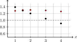
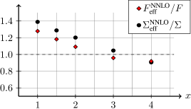
$(a_{x})$		$(b_{x})$

Figure 1: Finite-volume corrections to $\Sigma$ and $F$ at NNLO for geometries $(a_{x})$ and $(b_{x})$ at $m_{\pi}^{2}\sqrt{V}=1$, $F=90$ MeV, and $L=1.71$ fm.

In Figure 1 we visualize the NNLO results of Table 2. We confirm the picture obtained in Ref. [15] at NLO that the finite-volume corrections to $F$ can be largely reduced by an asymmetric lattice geometry with one appropriately large spatial dimension instead of one large temporal dimension.

We now turn to the non-universal terms that cannot be mapped to RMT. It follows from Eqs. (2.3) and (2.3) that the coefficients $\Upsilon_{4},\ldots,\Upsilon_{8}$ are independent of the choice of lattice geometry $(a_{x})$ or $(b_{x})$ for the same value of $x$. The coefficients $\Upsilon_{1}$, $\Upsilon_{2}$, and $\Upsilon_{3}$, however, are affected by the choice of lattice geometry $(a_{x})$ or $(b_{x})$, and we have

$$\Upsilon_{1},\Upsilon_{2},\Upsilon_{3}\propto P^{r}_{4}+4P^{r}_{5}\,.$$ (41)

We give values for $P^{r}_{4}+4P^{r}_{5}$ in Figure 2 at scale $\mu=V^{-1/4}$ for lattice geometries $(a_{x})$ and $(b_{x})$.

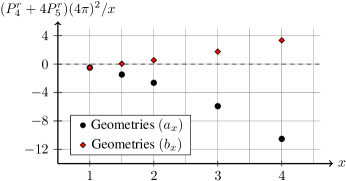
Figure 2: Linear combination of shape coefficients $P^{r}_{4}+4P^{r}_{5}$ for different geometries at scale $\mu=V^{-1/4}$. We divide by $x$ since $V=xL^{4}$ in Eq. (2.3).

Note that the non-universal contribution of $\Upsilon_{1}$, $\Upsilon_{2}$, and $\Upsilon_{3}$ is reduced significantly in lattice geometry $(b_{x})$ compared to lattice geometry $(a_{x})$ for the same value of $x$. In an upcoming publication [12] we perform the corresponding lattice simulation for $x=2$ and show numerically that the systematic deviations from RMT are indeed smaller for lattice geometry $(b_{2})$ compared to lattice geometry $(a_{2})$.

4 Conclusions

We discussed the $\varepsilon$-expansion at NNLO and determined the finite-volume effective action and the finite-volume effective LECs and HECs to this order. In the special case of two dynamical quarks confined to an asymmetric box we have confirmed the picture obtained at NLO that finite-volume corrections to the LECs $\Sigma$ and $F$ can be significantly reduced by choosing one appropriately large spatial dimension instead of a large temporal dimension, see Ref. [15]. Furthermore, we have shown that the systematic deviations from random matrix theory can also be reduced in the setup with one large spatial dimension. This implies that in order to determine the LECs $\Sigma$ and $F$ from eigenvalue correlation functions, as suggested in Refs. [6, 7] and performed in a pilot study in Ref. [23], one should choose an asymmetric lattice with one large spatial dimension. This will be demonstrated numerically in an upcoming publication [12].

We would like to add that even though we did not explicitly perform our calculations in a partially quenched setup, it is straightforward to extend our results to the partially quenched case, see, e.g., Ref. [15] for a discussion at NLO, and we expect our findings to be unmodified by the presence of valence quarks.

Appendix A The massless sunset diagram at finite volume

In this section we calculate the two-loop contribution defined by

$$P_{6} =V\int d^{d}x[\partial_{0}^{2}\bar{G}(x)]\bar{G}(x)^{2}=-\frac{1}{V}\sum_{k\neq 0}\frac{k_{0}^{2}}{k^{2}}\sum_{p\neq 0,-k}\frac{1}{p^{2}(p+k)^{2}}\,,$$ (42)

where the sum is over all nonzero momenta $k$ and $p$ with $p+k\neq 0$, and $k_{0}$ is the temporal component of the momentum vector $k$. We first express the propagators without constant mode as the limit of ordinary, massive propagators,

$$P_{6}=\lim_{m\to 0}P_{6}(m^{2})=\lim_{m\to 0}\left[P_{6}^{0}(m^{2})+P_{6}^{1}(m^{2})\right]$$ (43)

with

$$P_{6}^{0}(m^{2}) =\frac{2}{m^{2}V}\sum_{k}\frac{k_{0}^{2}}{(k^{2}+m^{2})^{2}}\,,$$

$$P_{6}^{1}(m^{2}) =-\frac{1}{V}\sum_{k,p}\frac{k_{0}^{2}}{(p^{2}+m^{2})[(p+k)^{2}+m^{2}](k^{2}+m^{2})}\,.$$ (44)

The terms $P_{6}^{0}(m^{2})$ and $P_{6}^{1}(m^{2})$ are calculated separately in the following.

A.1 The term $P_{6}^{0}(m^{2})$

We partition the term $P_{6}^{0}(m^{2})$ into its infinite-volume part and the finite-volume propagator $g_{1}$ defined in Eq. (2.3). We find

$$P_{6}^{0}(m^{2}) =\frac{2}{m^{2}V}\sum_{k}\frac{k_{0}^{2}}{(k^{2}+m^{2})^{2}}=\frac{1}{m^{2}}\partial_{\tilde{L}_{0}}\biggl{(}\tilde{L}_{0}\frac{1}{V}\sum_{k}\frac{1}{k^{2}+m^{2}}\biggr{)}$$

$$=\frac{1}{m^{2}}\frac{1}{(4\pi)^{d/2}}\Gamma(1-d/2)(m^{2})^{d/2-1}+\frac{1}{m^{2}}g_{1}(m^{2})+\frac{1}{m^{2}}\tilde{L}_{0}\partial_{\tilde{L}_{0}}g_{1}(m^{2})\,,$$ (45)

where

$$g_{1}(m^{2}) =\frac{1}{Vm^{2}}-\frac{\beta_{1}}{\sqrt{V}}-\frac{m^{2}\log(m^{2}\sqrt{V})}{(4\pi)^{2}}-m^{2}\beta_{2}+{\cal O}(m^{4})\,.$$ (46)

Therefore we can express $P_{6}^{0}(m^{2})$ in terms of $\beta_{1}$, $\beta_{2}$, and $\lambda$ as

$$P_{6}^{0}(m^{2}) =2\lambda-\frac{1}{m^{2}\sqrt{V}}\tilde{L}_{0}\partial_{\tilde{L}_{0}}\beta_{1}-\frac{\beta_{1}}{2m^{2}\sqrt{V}}-\frac{\log\sqrt{V}}{(4\pi)^{2}}-\partial_{\tilde{L}_{0}}(\tilde{L}_{0}\beta_{2})-\frac{1}{2(4\pi)^{2}}+{\cal O}(m^{2})\,.$$ (47)

A.2 The term $P_{6}^{1}(m^{2})$

The second term

$$P_{6}^{1}(m^{2}) =-\frac{1}{V}\sum_{k}\frac{k_{0}^{2}}{k^{2}+m^{2}}\sum_{p}\frac{1}{(p^{2}+m^{2})[(p+k)^{2}+m^{2}]}$$ (48)

is more involved. We use Poisson’s summation formula

$$\sum_{n=-\infty}^{\infty}e^{2\pi in\varphi}=\sum_{n=-\infty}^{\infty}\delta(\varphi-n)$$ (49)

and write

$$P_{6}^{1}(m^{2})=-V\sum_{r,s}\int\frac{d^{d}k}{(2\pi)^{d}} \frac{d^{d}p}{(2\pi)^{d}}\exp\biggl{[}i\sum_{j}\tilde{L}_{j}(r_{j}k_{j}+s_{j}p_{j})\biggr{]}$$

$$\times\frac{k_{0}^{2}}{(p^{2}+m^{2})[(p+k)^{2}+m^{2}](k^{2}+m^{2})}\,,$$ (50)

where the sum is over $r,s\in\mathbbm{Z}^{4}$. We partition the sum over $r$ and $s$ into

$$(A) \qquad r=0\land s=0\,,$$

$$(B) \qquad r\neq 0\land s=0\,,$$

$$(C) \qquad r=0\land s\neq 0\,,$$

$$(D) \qquad r\neq 0\land s\neq 0\land s=r\,,$$

$$(E) \qquad r\neq 0\land s\neq 0\land s\neq r\,.$$ (51)

Part (A) is given by the infinite-volume sunset diagram, see Ref. [24], which scales with $Vm^{d}$ and therefore vanishes in the massless limit. The parts $P_{6}^{1B}(m^{2}),\ldots,P_{6}^{1E}(m^{2})$ are calculated in the following.

A.2.1 The term $P_{6}^{1B}(m^{2})$

Along the lines of Eqs. (A.10) and (A.11) of Ref. [25] we separate

$$P_{6}^{1B}(m^{2}) =P_{6}^{1B1}(m^{2})+P_{6}^{1B2}(m^{2})$$ (52)

with

$$P_{6}^{1B1}(m^{2}) =-V\sum_{r\neq 0}\int\frac{d^{d}k}{(2\pi)^{d}}\frac{d^{d}p}{(2\pi)^{d}}\frac{k_{0}^{2}}{k^{2}+m^{2}}\frac{1}{(p^{2}+m^{2})^{2}}\exp\biggl{(}i\sum_{j}\tilde{L}_{j}r_{j}k_{j}\biggr{)},$$

$$P_{6}^{1B2}(m^{2}) =-V\sum_{r\neq 0}\int\frac{d^{d}k}{(2\pi)^{d}}\frac{d^{d}p}{(2\pi)^{d}}\frac{k_{0}^{2}}{k^{2}+m^{2}}\exp\biggl{(}i\sum_{j}\tilde{L}_{j}r_{j}k_{j}\biggr{)}$$

$$\quad\times\biggl{[}\frac{1}{(p^{2}+m^{2})[(p+k)^{2}+m^{2}]}-\frac{1}{(p^{2}+m^{2})^{2}}\biggr{]}\,.$$ (53)

The term $P_{6}^{1B1}(m^{2})$ contains the ultraviolet divergence and can be calculated explicitly,

$$P_{6}^{1B1}(m^{2}) =-V\int\frac{d^{d}p}{(2\pi)^{d}}\frac{1}{(p^{2}+m^{2})^{2}}\sum_{r\neq 0}\int\frac{d^{d}k}{(2\pi)^{d}}\frac{k_{0}^{2}}{k^{2}+m^{2}}\exp\biggl{(}i\sum_{j}\tilde{L}_{j}r_{j}k_{j}\biggr{)}$$

$$=-2\lambda P_{1}-\frac{1+\log m^{2}}{(4\pi)^{2}}P_{1}+{\cal O}(Vm^{d})\,,$$ (54)

where $P_{1}$ is the one-loop shape coefficient defined in Eq. (2.3). The term $P_{6}^{1B2}(m^{2})$ is finite. After a tedious but straightforward calculation along the lines of Ref. [19] we can express $P_{6}^{1B2}(m^{2})$ as

$$P_{6}^{1B2}(m^{2})=-\frac{1}{(8\pi)^{2}}\sum_{r\neq 0}\int_{0}^{\infty}dxdydz\>K(x,y,z)\>\exp\biggl{[}-(x+y+z)\frac{m^{2}\sqrt{V}}{4\pi}\biggr{]}$$ (55)

with

$$K(x,y,z) =\frac{1}{(xy+xz+yz)^{3}}\biggl{[}2(x+y)-\frac{({\tilde{L}_{0}}^{2}/\sqrt{V})[2r_{0}(x+y)]^{2}\pi}{(yz+xy+xz)}\biggr{]}$$

$$\quad\times\exp\biggl{[}-\sum_{j}\frac{({\tilde{L}_{j}}^{2}/\sqrt{V})r_{j}^{2}(x+y)\pi}{(yz+xy+xz)}\biggr{]}$$

$$\quad-\frac{1}{(x+y)^{2}z^{3}}\Bigl{[}2-({\tilde{L}_{0}}^{2}/\sqrt{V})4\pi r_{0}^{2}/z\Bigr{]}\exp\biggl{[}-\sum_{j}({\tilde{L}_{j}}^{2}/\sqrt{V})\pi\frac{r_{j}^{2}}{z}\biggr{]}\,.$$ (56)

This expression is suitable for a numerical evaluation of $P_{6}^{1B2}(m^{2})$ if we perform the integral over $x$, $y$ and $z$ in spherical coordinates. In Sec. A.2.4 we discuss how to efficiently calculate infinite sums such as the sums over $r_{0},\ldots,r_{3}$ with $r\neq 0$ in Eq. (55).

A.2.2 The term $P_{6}^{1C}(m^{2})$

The method used to separate the divergent part of $P_{6}^{1B}(m^{2})$ does not work for the integral over $k$ since it has a power divergence. Nevertheless, we can calculate the divergent sub-diagram

$$I_{\mu\nu}(m,p) =\int\frac{d^{d}k}{(2\pi)^{d}}\frac{k_{\mu}k_{\nu}}{(k^{2}+m^{2})[(p+k)^{2}+m^{2}]}$$ (57)

explicitly. The result is given by [26]

$$I_{\mu\nu}(m,p) =g_{\mu\nu}\int_{0}^{1}dx\frac{[m^{2}+x(1-x)p^{2}]\log[m^{2}+x(1-x)p^{2}]}{2(4\pi)^{2}}$$

$$\quad-p_{\mu}p_{\nu}\int_{0}^{1}dx\frac{x^{2}}{(4\pi)^{2}}\bigl{[}1+\log[m^{2}+x(1-x)p^{2}]\bigr{]}$$

$$\quad+g_{\mu\nu}\lambda\biggl{(}\frac{1}{6}p^{2}+m^{2}\biggr{)}-\frac{2}{3}\lambda p_{\mu}p_{\nu}\,.$$ (58)

We can thus separate the divergent part of

$$P_{6}^{1C}(m^{2}) =-V\sum_{s\neq 0}\int\frac{d^{d}p}{(2\pi)^{d}}\frac{I_{00}(m,p)}{p^{2}+m^{2}}\exp\biggl{(}i\sum_{j}\tilde{L}_{j}s_{j}p_{j}\biggr{)}\,,$$ (59)

which is given by

$$[P_{6}^{1C}(m^{2})]_{\text{UV}} =-\frac{\lambda V}{6}\sum_{s\neq 0}\int\frac{d^{d}p}{(2\pi)^{d}}\frac{(p^{2}+m^{2})+5m^{2}-4p_{0}^{2}}{p^{2}+m^{2}}\exp\biggl{(}i\sum_{j}\tilde{L}_{j}s_{j}p_{j}\biggr{)}$$

$$=-\frac{5}{6}\lambda-\frac{2}{3}\lambda P_{1}+{\cal O}(m^{2})\,.$$ (60)

In the calculation of $[P_{6}^{1C}(m^{2})]_{\text{UV}}$ we used the identities

$$V\sum_{s\neq 0}\int\frac{d^{d}p}{(2\pi)^{d}}\frac{1}{p^{2}+m^{2}}\exp\biggl{(}i\sum_{j}\tilde{L}_{j}s_{j}p_{j}\biggr{)} =\frac{1}{m^{2}}+{\cal O}(m^{0})\,,$$

$$\sum_{s\neq 0}\int\frac{d^{d}p}{(2\pi)^{d}}\>\exp\biggl{(}i\sum_{j}\tilde{L}_{j}s_{j}p_{j}\biggr{)} =0\,,$$

$$\sum_{s\neq 0}\int\frac{d^{d}p}{(2\pi)^{d}}\frac{p_{0}^{2}}{p^{2}+m^{2}}\exp\biggl{(}i\sum_{j}\tilde{L}_{j}s_{j}p_{j}\biggr{)} =-P_{1}+{\cal O}(m^{d})\,.$$ (61)

Note that the first two identities hold for arbitrary $d$. Thus there is no finite contribution from the product of these integrals with $\lambda$.

The finite contributions to $P_{6}^{1C}(m^{2})$ are given by

$$[P_{6}^{1C}(m^{2})]_{\text{finite}} =-\frac{V}{2(4\pi)^{2}}\sum_{s\neq 0}J^{\prime}_{s}(m^{2})\,,$$ (62)

where

$$J^{\prime}_{s}(m^{2})=\int_{0}^{1}dx\int\frac{d^{4}p}{(2\pi)^{4}}\frac{{\cal F}_{1}(m^{2},p^{2})-p_{0}^{2}{\cal F}_{2}(m^{2},p^{2})}{p^{2}+m^{2}}\exp\biggl{(}i\sum_{j}\tilde{L}_{j}s_{j}p_{j}\biggr{)}$$ (63)

with

$${\cal F}_{1}(m^{2},p^{2}) =[m^{2}+x(1-x)p^{2}]\log[m^{2}+x(1-x)p^{2}]\,,$$

$${\cal F}_{2}(m^{2},p^{2}) =2x^{2}\big{(}1+\log[m^{2}+x(1-x)p^{2}]\big{)}\,.$$ (64)

We define $L^{s}_{i}=\tilde{L}_{i}s_{i}$ and rotate the coordinate system of $p$ such that

$$J^{\prime}_{s}(m^{2}) =\int_{0}^{1}dx\int\frac{d^{4}p}{(2\pi)^{4}}\frac{{\cal F}_{1}(m^{2},p^{2})+(1/{\tilde{L}_{0}}^{2}){\cal F}_{2}(m^{2},p^{2})\partial_{s_{0}}^{2}}{p^{2}+m^{2}}\exp(iL^{s}p_{0})$$ (65)

with $L^{s}=[\sum_{n=0}^{3}(L^{s}_{n})^{2}]^{1/2}$. After differentiating w.r.t. $s_{0}$ we find

$$J^{\prime}_{s}(m^{2}) =\int_{0}^{1}dx\int\frac{d^{4}p}{(2\pi)^{4}}\frac{[{\cal F}_{1}(m^{2},p^{2})+{\cal F}_{2}(m^{2},p^{2}){\cal G}_{s}(p_{0}V^{1/4})]\exp(iL^{s}p_{0})}{\Bigl{(}p_{0}-i\sqrt{p_{\perp}^{2}+m^{2}}\Bigr{)}\Bigl{(}p_{0}+i\sqrt{p_{\perp}^{2}+m^{2}}\Bigr{)}}$$ (66)

with

$${\cal G}_{s}(p_{0}V^{1/4}) =\frac{ip_{0}}{L^{s}}-\frac{ip_{0}s_{0}^{2}\tilde{L}_{0}^{2}}{(L^{s})^{3}}-\frac{p_{0}^{2}s_{0}^{2}\tilde{L}_{0}^{2}}{(L^{s})^{2}}$$ (67)

and

$$p^{2}=p_{0}^{2}+p_{\perp}^{2}\,.$$ (68)

In Figure 3 we sketch the structure of the integrand of Eq. (66) in the complex plane.

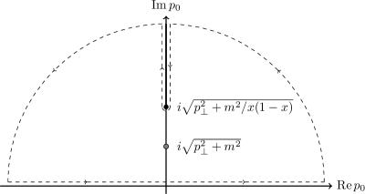
Figure 3: The complex plane of $p_{0}$.

There are two poles at $p_{0}=\pm i\sqrt{p_{\perp}^{2}+m^{2}}$ and a branch cut due to the logarithms in ${\cal F}_{1}(m^{2},p^{2})$ and ${\cal F}_{2}(m^{2},p^{2})$. We can close the integration contour in the upper half-plane and find

$$J^{\prime}_{s}(m^{2})=[J^{\prime}_{s}(m^{2})]_{p}+[J^{\prime}_{s}(m^{2})]_{c}\,,$$ (69)

where $[J^{\prime}_{s}(m^{2})]_{p}$ is the contribution of the pole and $[J^{\prime}_{s}(m^{2})]_{c}$ is the contribution of the branch cut. The contribution of the pole is given by

$$[J^{\prime}_{s}(m^{2})]_{p} =\frac{1}{(2\pi)^{2}V}\int_{0}^{1}dx\int_{0}^{\infty}d\hat{p}_{\perp}\hat{p}^{2}_{\perp}\exp\Bigl{(}-l^{s}\sqrt{\hat{p}_{\perp}^{2}+m^{2}\sqrt{V}}\Bigr{)}$$

$$\quad\times\frac{{\cal F}_{1}(m^{2},-m^{2})\sqrt{V}+{\cal F}_{2}(m^{2},-m^{2}){\cal G}_{s}\Bigl{(}i\sqrt{\hat{p}_{\perp}^{2}+m^{2}\sqrt{V}}\Bigr{)}\sqrt{V}}{\sqrt{\hat{p}_{\perp}^{2}+m^{2}\sqrt{V}}}$$ (70)

with $l^{s}=L^{s}/V^{1/4}$ and $\hat{p}_{\perp}=p_{\perp}V^{1/4}$. The contribution of the branch cut is given by

$$[J^{\prime}_{s}(m^{2})]_{c}=\frac{1}{(2\pi)^{4}}\int_{0}^{1}dx \int d^{3}p_{\perp}\int_{i\sqrt{p_{\perp}^{2}+m^{2}/x(1-x)}}^{i\infty}dp_{0}\exp(iL^{s}p_{0})$$

$$\times\frac{\operatorname{Disc}{\cal F}_{1}(m^{2},p^{2})+\operatorname{Disc}{\cal F}_{2}(m^{2},p^{2}){\cal G}_{s}(p_{0}V^{1/4})}{p^{2}+m^{2}}\,,$$ (71)

where

$$\operatorname{Disc}{\cal F}_{1}(m^{2},p^{2}) =\lim_{\varepsilon\to 0}\left[{\cal F}_{1}(p_{\perp}^{2}+(p_{0}+\varepsilon)^{2})-{\cal F}_{1}(p_{\perp}^{2}+(p_{0}-\varepsilon)^{2})\right]$$

$$=2\pi i[m^{2}+x(1-x)p^{2}]\,,$$

$$\operatorname{Disc}{\cal F}_{2}(m^{2},p^{2}) =\lim_{\varepsilon\to 0}\left[{\cal F}_{2}(p_{\perp}^{2}+(p_{0}+\varepsilon)^{2})-{\cal F}_{2}(p_{\perp}^{2}+(p_{0}-\varepsilon)^{2})\right]$$

$$=4\pi ix^{2}\,.$$ (72)

Therefore

$$[J^{\prime}_{s}(m^{2})]_{c}=\frac{2}{(2\pi)^{2}V} \int_{0}^{1}dx\int_{0}^{\infty}d\hat{p}_{\perp}\hat{p}_{\perp}^{2}\int_{\sqrt{\hat{p}_{\perp}^{2}+m^{2}\sqrt{V}/x(1-x)}}^{\infty}dy\exp(-l^{s}y)$$

$$\times\frac{m^{2}\sqrt{V}+x(1-x)(\hat{p}_{\perp}^{2}-y^{2})+2x^{2}{\cal G}_{s}(iy)\sqrt{V}}{y^{2}-\hat{p}_{\perp}^{2}-m^{2}\sqrt{V}}$$ (73)

with $p_{0}=iy$ and thus $dp_{0}=idy$. In Sec. 3 we calculate $[P_{6}^{1C}(m^{2})]_{\text{finite}}$ numerically at scale $\mu=V^{-1/4}$, i.e., we replace ${\cal F}_{1}(m^{2},p^{2})$ and ${\cal F}_{2}(m^{2},p^{2})$ by

$${\cal F}_{1}(m^{2},p^{2}) =[m^{2}+x(1-x)p^{2}]\log\bigl{[}m^{2}\sqrt{V}+x(1-x)p^{2}\sqrt{V}\bigr{]}\,,$$

$${\cal F}_{2}(m^{2},p^{2}) =2x^{2}\bigl{(}1+\log[m^{2}\sqrt{V}+x(1-x)p^{2}\sqrt{V}]\bigr{)}\,.$$ (74)

A.2.3 The term $P_{6}^{1D}(m^{2})$

The term $P_{6}^{1D}(m^{2})$ is equal to the term $P_{6}^{1C}(m^{2})$. This can be seen by shifting the integration variables $p_{\mu}\to p_{\mu}-k_{\mu}$ and using the invariance of the integral under $k_{\mu}\to-k_{\mu}$.

A.2.4 The term $P_{6}^{1E}(m^{2})$

The term $P_{6}^{1E}(m^{2})$ is finite and can be calculated numerically. We rewrite $P_{6}^{1E}(m^{2})$ analogously to $P_{6}^{1B2}(m^{2})$ as

$$P_{6}^{1E}(m^{2}) =-\frac{1}{(8\pi)^{2}}\sum_{r\neq 0,s\neq 0,r\neq s}\int_{0}^{\infty}dxdydz\>\frac{1}{(xy+xz+yz)^{3}}$$

$$\quad\times\biggl{[}2(x+y)-\frac{({\tilde{L}_{0}}^{2}/\sqrt{V})[-2s_{0}y+2r_{0}(x+y)]^{2}\pi}{yz+xy+xz}\biggr{]}$$

$$\quad\times\exp\biggl{[}-\sum_{j}\frac{({\tilde{L}_{j}}^{2}/\sqrt{V})[-2r_{j}s_{j}y+r_{j}^{2}(x+y)+s_{j}^{2}(y+z)]\pi}{yz+xy+xz}\biggr{]}$$

$$\quad\times\exp\biggl{[}-(x+y+z)\frac{m^{2}\sqrt{V}}{4\pi}\biggr{]}\,.$$ (75)

In the following we discuss how to efficiently calculate the infinite sums over $s_{0},\ldots,s_{3},r_{0},\ldots,r_{3}$. We first define

$$g =\sum_{r\neq 0,s\neq 0,r\neq s}\prod_{j=0}^{3}\exp(-a_{j}r_{j}^{2}-b_{j}s_{j}^{2}+c_{j}r_{j}s_{j}+d_{j}r_{j}+e_{j}s_{j})$$

$$=\sum_{s\neq 0}\biggl{[}\sum_{r}\prod_{j}\exp(-a_{j}r_{j}^{2}-b_{j}s_{j}^{2}+c_{j}r_{j}s_{j}+d_{j}r_{j}+e_{j}s_{j})-\prod_{j}\exp(-b_{j}s_{j}^{2}+e_{j}s_{j})$$

$$\qquad\quad\qquad-\prod_{j}\exp[-(a_{j}+b_{j}-c_{j})s_{j}^{2}+(d_{j}+e_{j})s_{j}]\biggr{]}$$

$$=2+\sum_{r,s}\prod_{j}\exp(-a_{j}r_{j}^{2}-b_{j}s_{j}^{2}+c_{j}r_{j}s_{j}+d_{j}r_{j}+e_{j}s_{j})-\sum_{s}\prod_{j}\exp(-b_{j}s_{j}^{2}+e_{j}s_{j})$$

$$\quad-\sum_{r}\prod_{j}\exp(-a_{j}r_{j}^{2}+d_{j}r_{j})-\sum_{s}\prod_{j}\exp[-(a_{j}+b_{j}-c_{j})s_{j}^{2}+(d_{j}+e_{j})s_{j}]\,,$$ (76)

where $a_{j},b_{j},c_{j},d_{j},e_{j}\in\mathbbm{C}$ with $\operatorname{Re}a_{j},\operatorname{Re}b_{j}>0$ and $j=0,\ldots,3$. In this way we can write

$$g =\prod_{j=0}^{3}\bar{g}(a_{j},b_{j},c_{j},d_{j},e_{j})-\prod_{j=0}^{3}\nu(b_{j},e_{j})-\prod_{j=0}^{3}\nu(a_{j},d_{j})-\prod_{j=0}^{3}\nu(a_{j}+b_{j}-c_{j},d_{j}+e_{j})+2\,,$$ (77)

where

$$\nu(a,b) =\sum_{n}\exp(-an^{2}+bn)\,,$$

$$\bar{g}(a,b,c,d,e) =\sum_{n,m}\exp(-an^{2}-bm^{2}+cmn+dn+em)$$

$$=\sum_{m}\nu(a,cm+d)\exp(-bm^{2}+em)\,.$$ (78)

Since $\nu$ is a Jacobi theta function it transforms covariantly under inversion of $a$,

$$\nu(a,b) =\sqrt{\frac{\pi}{a}}\exp(b^{2}/4a)\nu(\pi^{2}/a,i\pi(b/a))\,,$$ (79)

which is readily shown using Poisson’s summation formula. For $a\in\mathbbm{R}$ with $a<\pi$ we can therefore use Eq. (79) to achieve a swift convergence of the sum over $n$ in $\nu(a,b)$ in Eq. (A.2.4). In fact in the least favorable case of $a=\pi$ we need only to sum all $n$ with ${|n-n_{0}|}\leq 4$, where $n=n_{0}\in\mathbbm{Z}$ maximizes $-an^{2}+bn$, to achieve a precision of $-\log_{10}[\exp(-4^{2}\pi)]\approx 22$ digits. In this way we can express $P_{6}^{1E}(m^{2})$ as

$$P_{6}^{1E}(m^{2}) =-\frac{1}{(8\pi)^{2}}\int_{0}^{\infty}dxdydz\>R^{3}\left[2(x+y)-R\tilde{l}_{0}^{2}[-2y\partial_{e_{0}}+2(x+y)\partial_{d_{0}}]^{2}\pi\right]$$

$$\quad\times g(e_{0},d_{0})\Big{|}_{e_{0}=d_{0}=0}\exp\biggl{[}-(x+y+z)\frac{m^{2}\sqrt{V}}{4\pi}\biggr{]}$$ (80)

with

$$R =\frac{1}{yz+xy+xz}\,, \tilde{l}_{j} =\tilde{L}_{j}/V^{1/4}\,,$$

$$a_{j} =R\tilde{l}_{j}^{2}(x+y)\pi\,, b_{j} =R\tilde{l}_{j}^{2}(y+z)\pi\,,$$

$$c_{j} =R\tilde{l}_{j}^{2}2\pi y\,, d_{1} =d_{2}=d_{3}=e_{1}=e_{2}=e_{3}=0\,.$$ (81)

The integral over $x$, $y$ and $z$ can be performed conveniently in spherical coordinates, as in the case of $P_{6}^{1B2}(m^{2})$.

A.3 The complete diagram

We combine all contributions to $P_{6}(m^{2})$ and find that the complete diagram at scale $\mu=V^{-1/4}$ is given by

$$(P_{6})_{\text{UV}} =\frac{1}{3}\lambda-\frac{10}{3}\lambda P_{1}\,,$$

$$P_{6}^{r}(m^{2}) =-\frac{1}{m^{2}\sqrt{V}}\tilde{L}_{0}\partial_{\tilde{L}_{0}}\beta_{1}-\frac{\beta_{1}}{2m^{2}\sqrt{V}}-\frac{\log(m^{2}\sqrt{V})}{(4\pi)^{2}}P_{1}-\partial_{\tilde{L}_{0}}(\tilde{L}_{0}\beta_{2})$$

$$\quad-\frac{1}{2(4\pi)^{2}}+2[P_{6}^{1C}(m^{2})]_{\text{finite}}-\frac{1}{(4\pi)^{2}}P_{1}+P_{6}^{1B2}(m^{2})+P_{6}^{1E}(m^{2})\,,$$

$$P_{6}^{r} =\lim_{m^{2}\to 0}P_{6}^{r}(m^{2})\,,$$ (82)

where $P_{6}^{r}$ is the renormalized shape coefficient at scale $\mu=V^{-1/4}$. In Figs. 4 and 5 we show the result of a numerical calculation of $P_{6}^{r}(m^{2})$ for different values of $m^{2}\sqrt{V}$.

Note that the linear divergences as well as the logarithmic divergences in $1/m^{2}\sqrt{V}$ cancel. We perform a fit to a polynomial of order four for different ranges of $m^{2}\sqrt{V}$: (i) $m^{2}\sqrt{V}<0.75$, (ii) $m^{2}\sqrt{V}<1.5$, and (iii) $m^{2}\sqrt{V}<3$. The result of the fits and the corresponding extrapolated values for $m^{2}=0$ are given in Table 3.

	D..4(i)	D..4(ii)	D..4(iii)	extrapolation
$(a_{1})$	$-0.010591$	$-0.010538$	$-0.010501$	$-0.0106(1)$
$(a_{3/2})$	$0.009395$	$0.009429$	$0.009439$	$0.00940(4)$
$(a_{2})$	$0.024867$	$0.024892$	$0.024884$	$0.02487(2)$
$(a_{3})$	$0.031944$	$0.031799$	$0.031778$	$0.0319(1)$
$(a_{4})$	$-0.021362$	$-0.021531$	$-0.021720$	$-0.0214(3)$
$(b_{3/2})$	$-0.015129$	$-0.015092$	$-0.015050$	$-0.01513(3)$
$(b_{2})$	$-0.015765$	$-0.015714$	$-0.015669$	$-0.01577(7)$
$(b_{3})$	$-0.008005$	$-0.007968$	$-0.007904$	$-0.0080(1)$
$(b_{4})$	$0.011724$	$0.011748$	$0.011810$	$0.0117(1)$

Table 3: Best fit of $P_{6}^{r}$ for regions (i), (ii), and (iii) and extrapolated values of $P_{6}^{r}$ for different geometries.

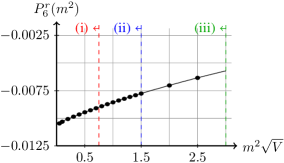
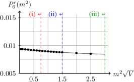
$(a_{1})$	$(a_{3/2})$
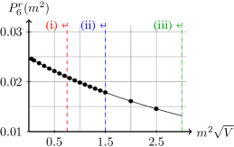
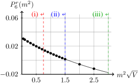
$(a_{2})$	$(a_{3})$
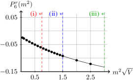
$(a_{4})$

Figure 4: Extrapolation of $P^{r}_{6}=\lim_{m\to 0}P^{r}_{6}(m^{2})$ for lattice geometries $(a_{x})$, $x\in\{1,3/2,2,3,4\}$ at scale $\mu=V^{-1/4}$. We fit a polynomial of order four including numerical data from three different ranges (i), (ii), and (iii).

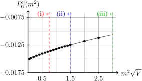
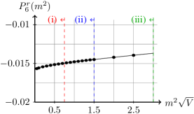
$(b_{3/2})$	$(b_{2})$
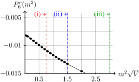
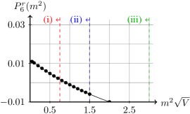
$(b_{3})$	$(b_{4})$

Figure 5: Extrapolation of $P^{r}_{6}=\lim_{m\to 0}P^{r}_{6}(m^{2})$ for lattice geometries $(b_{x})$, $x\in\{3/2,2,3,4\}$ at scale $\mu=V^{-1/4}$. We fit a polynomial of order four including numerical data from three different ranges (i), (ii), and (iii).

References

- [1] J. Gasser and H. Leutwyler, Thermodynamics of chiral symmetry, Phys. Lett. B188 (1987) 477.
- [2] E. V. Shuryak and J. J. M. Verbaarschot, Random matrix theory and spectral sum rules for the Dirac operator in QCD, Nucl. Phys. A560 (1993) 306–320, [hep-th/9212088].
- [3] J. J. M. Verbaarschot and T. Wettig, Random matrix theory and chiral symmetry in QCD, Ann. Rev. Nucl. Part. Sci. 50 (2000) 343–410, [hep-ph/0003017].
- [4] G. Akemann, Matrix models and QCD with chemical potential, Int. J. Mod. Phys. A22 (2007) 1077–1122, [hep-th/0701175].
- [5] F. Basile and G. Akemann, Equivalence of QCD in the epsilon-regime and chiral random matrix theory with or without chemical potential, JHEP 12 (2007) 043, [arXiv:0710.0376].
- [6] P. H. Damgaard, U. M. Heller, K. Splittorff, and B. Svetitsky, A new method for determining F(pi) on the lattice, Phys. Rev. D72 (2005) 091501, [hep-lat/0508029].
- [7] G. Akemann, P. H. Damgaard, J. C. Osborn, and K. Splittorff, A new chiral two-matrix theory for Dirac spectra with imaginary chemical potential, Nucl. Phys. B766 (2007) 34–67, [hep-th/0609059].
- [8] T. Mehen and B. C. Tiburzi, Quarks with twisted boundary conditions in the epsilon regime, Phys. Rev. D72 (2005) 014501, [hep-lat/0505014].
- [9] JLQCD Collaboration, H. Fukaya et. al., Two-flavor lattice QCD simulation in the epsilon-regime with exact chiral symmetry, Phys. Rev. Lett. 98 (2007) 172001, [hep-lat/0702003].
- [10] H. Fukaya et. al., Two-flavor lattice QCD in the epsilon-regime and chiral random matrix theory, Phys. Rev. D76 (2007) 054503, [arXiv:0705.3322].
- [11] JLQCD Collaboration, H. Fukaya et. al., Determination of the chiral condensate from 2+1-flavor lattice QCD, Phys. Rev. Lett. 104 (2010) 122002, [arXiv:0911.5555].
- [12] C. Lehner, J. Bloch, S. Hashimoto, and T. Wettig, “The Dirac eigenvalue spectrum and the low-energy constants and .” In preparation.
- [13] P. H. Damgaard, T. DeGrand, and H. Fukaya, Finite-volume correction to the pion decay constant in the epsilon-regime, JHEP 12 (2007) 060, [arXiv:0711.0167].
- [14] G. Akemann, F. Basile, and L. Lellouch, Finite size scaling of meson propagators with isospin chemical potential, JHEP 12 (2008) 069, [arXiv:0804.3809].
- [15] C. Lehner and T. Wettig, Partially quenched chiral perturbation theory in the epsilon regime at next-to-leading order, JHEP 11 (2009) 005, [arXiv:0909.1489].
- [16] F. C. Hansen, Finite size effects in spontaneously broken SU(N) SU(N) theories, Nucl. Phys. B345 (1990) 685–708.
- [17] J. Gasser and H. Leutwyler, Chiral perturbation theory: Expansions in the mass of the strange quark, Nucl. Phys. B250 (1985) 465.
- [18] J. Bijnens, G. Colangelo, and G. Ecker, Renormalization of chiral perturbation theory to order p**6, Annals Phys. 280 (2000) 100–139, [hep-ph/9907333].
- [19] P. Hasenfratz and H. Leutwyler, Goldstone boson related finite size effects in field theory and critical phenomena with O(N) symmetry, Nucl. Phys. B343 (1990) 241–284.
- [20] J. Bijnens, Chiral perturbation theory beyond one loop, Prog. Part. Nucl. Phys. 58 (2007) 521–586, [hep-ph/0604043].
- [21] M. Abramowitz and I. A. Stegun, Handbook of Mathematical Functions with Formulas, Graphs, and Mathematical Tables. Dover, New York, ninth Dover printing, tenth GPO printing ed., 1964.
- [22] J. Gasser and H. Leutwyler, Chiral perturbation theory to one loop, Ann. Phys. 158 (1984) 142.
- [23] T. DeGrand and S. Schaefer, Parameters of the lowest order chiral Lagrangian from fermion eigenvalues, Phys. Rev. D76 (2007) 094509, [arXiv:0708.1731].
- [24] G. Amoros, J. Bijnens, and P. Talavera, Two-point functions at two loops in three flavour chiral perturbation theory, Nucl. Phys. B568 (2000) 319–363, [hep-ph/9907264].
- [25] G. Colangelo and C. Haefeli, Finite volume effects for the pion mass at two loops, Nucl. Phys. B744 (2006) 14–33, [hep-lat/0602017].
- [26] G. Passarino and M. J. G. Veltman, One loop corrections for e+ e- annihilation into mu+ mu- in the Weinberg model, Nucl. Phys. B160 (1979) 151.