Kochen-Specker Sets and
Generalized Orthoarguesian Equations

Abstract.

Every set (finite or infinite) of quantum vectors (states) satisfies generalized orthoarguesian equations ($n$OA). We consider two 3-dim Kochen-Specker (KS) sets of vectors and show how each of them should be represented by means of a Hasse diagram—a lattice, an algebra of subspaces of a Hilbert space–that contains rays and planes determined by the vectors so as to satisfy $n$OA. That also shows why they cannot be represented by a special kind of Hasse diagram called a Greechie diagram, as has been erroneously done in the literature. One of the KS sets (Peres’) is an example of a lattice in which 6OA pass and 7OA fails, and that closes an open question of whether the 7oa class of lattices properly contains the 6oa class. This result is important because it provides additional evidence that our previously given proof of $n{\rm oa}\subseteq(n+1){\rm oa}$ can be extended to proper inclusion $n{\rm oa}\subset(n+1){\rm oa}$ and that $n{\rm OA}$ form an infinite sequence of successively stronger equations.

1. Introduction

Many authors have tried to empirically justify the mathematically well-established orthoisomorphism between the so-called Hilbert lattice and the lattice of subspaces of a Hilbert space, which has been worked out by many authors over the last 75 years.[1, 2, 3] However, a missing link between empirical quantum measurements and its lattice structure was a proper description of a correspondence between the standard quantum measurements, which use Hilbert vectors and states, on the one hand, and Hilbert lattices (algebras of the closed subspaces of Hilbert space), which make use of subspaces that contain these vectors and/or are spanned by them, on the other. What hampered a search for such a correspondence was a too narrow focus on orthogonality and on infinite-dimensionality via Greechie lattices (meaning the lattices depicted by Greechie diagrams). In Ref. [4] we gave two examples: empirical reconstruction of quantum mechanics via lattice theory and a description of Kochen-Specker’s setups via lattice theory.

A lattice can correctly represent a given formal description of a quantum system only if it satisfies all the equations that the lattice of subspaces of a Hilbert space satisfies. The only known set of equations that are related to the algebraic structure of the latter lattice (i.e., excluding those that are related to states introduced on the lattice) are the generalized orthoarguesian equations ($n$OA, $n\geq 3$). [33] Thus, these equations are an essential tool for analysing lattices for particular experimental setups. If a lattice does not pass $n$OA for all $n$, then it is not a correct lattice.

In this paper, we analyze two Kochen-Specker (KS) setups: Bub’s [5] and Peres’ [6]. We represent them by MMP hypergraphs. Vectors correspond to vertices in MMP hypergraphs, and tetrads of orthogonal vectors correspond to edges in MMP hypergraphs. MMP hypergraphs (also called MMP diagrams) are defined in Ref. [7] and in Sec. 2. One can establish a correspondence between MMP hypergraphs and lattices of subspaces of a Hilbert space. In such lattices the vertices of MMP hypergraphs correspond to lattice atoms and their edges to lattice blocks. Thus any KS setup can eventually be represented by a lattice.

In Sec. 3, we first show why KS setups cannot be represented by a special kind of lattice, called Greechie lattices, as erroneously claimed in the literature. Then we explain how they can be represented for use with any specifically chosen Hilbert lattice equation. In doing so, we introduce a new kind of lattice—we call it MMPL—that represents all nonorthogonal lattice elements as well as their meets and joins that take place in a proof of the chosen equation. As specific examples, we consider the 3OA equation for Bub’s KS lattice and 7OA for Peres’.

We show that Peres’ lattice satisfies 3OA through 6OA but violates 7OA. In Sec. 4, we then generate a serious of other lattices with this property. In Ref. [8], we proved that all individual orthoarguesian equations found previously (by other authors) were equivalent to either 3OA or 4OA and showed lattices in which 3OA and 4OA passed but 5OA failed. In Ref. [9], we found lattices in which 6OA failed and OAs up to 5OA passed.

Therefore, our finding of a series of lattices that satisfy 3OA-6OA but fail in 7OA amounts to a very strong indication that $n$oa’s properly contain each other for successively increasing $n$, for all $n$.

2. Lattice Definitions and Theorems

The closed subspaces of a Hilbert space form an algebra called a Hilbert lattice (defined by Def. 2.5). In any Hilbert lattice, the operation meet, $a\cap b$, corresponds to set intersection, ${\mathcal{H}}_{a}\bigcap{\mathcal{H}}_{b}$, of subspaces ${\mathcal{H}}_{a},{\mathcal{H}}_{b}$ of Hilbert space ${\mathcal{H}}$, the ordering relation $a\leq b$ corresponds to ${\mathcal{H}}_{a}\subseteq{\mathcal{H}}_{b}$, the operation join, $a\cup b$, corresponds to the smallest closed subspace of $\mathcal{H}$ containing ${\mathcal{H}}_{a}\bigcup{\mathcal{H}}_{b}$, and the orthocomplement $a^{\prime}$ corresponds to ${\mathcal{H}}_{a}^{\perp}$, the set of vectors orthogonal to all vectors in ${\mathcal{H}}_{a}$. Within Hilbert space there is also an operation which has no parallel in the Hilbert lattice: the sum of two subspaces ${\mathcal{H}}_{a}+{\mathcal{H}}_{b}$, which is defined as the set of sums of vectors from ${\mathcal{H}}_{a}$ and ${\mathcal{H}}_{b}$. We also have ${\mathcal{H}}_{a}+{\mathcal{H}}_{a}^{\perp}={\mathcal{H}}$. One can define all the lattice operations on a Hilbert space itself following the above definitions (${\mathcal{H}}_{a}\cap{\mathcal{H}}_{b}={\mathcal{H}}_{a}\bigcap{\mathcal{H}}_{b}$, etc.). Thus we have ${\mathcal{H}}_{a}\cup{\mathcal{H}}_{b}=\overline{{\mathcal{H}}_{a}+{\mathcal{H}}_{b}}=({\mathcal{H}}_{a}+{\mathcal{H}}_{b})^{\perp\perp}=({\mathcal{H}}_{a}^{\perp}\bigcap{\mathcal{H}}_{b}^{\perp})^{\perp}$,[10, p. 175] where $\overline{{\mathcal{H}}_{c}}$ is the closure of ${\mathcal{H}}_{c}$, and therefore ${\mathcal{H}}_{a}+{\mathcal{H}}_{b}\subseteq{\mathcal{H}}_{a}\cup{\mathcal{H}}_{b}$. When ${\mathcal{H}}$ is finite-dimensional or when the closed subspaces ${\mathcal{H}}_{a}$ and ${\mathcal{H}}_{b}$ are orthogonal to each other then ${\mathcal{H}}_{a}+{\mathcal{H}}_{b}={\mathcal{H}}_{a}\cup{\mathcal{H}}_{b}$. [11, pp. 21-29],   [12, pp. 66,67],  [13, pp. 8-16]

We briefly recall the definitions we will need. For further information, see Refs. [14, 8, 15, 9].

Definition 2.1.

[16] A lattice is an algebra ${\rm L}=\langle\mathcal{L}_{\rm O},\cap,\cup\rangle$ such that the following conditions are satisfied for any $a,b,c\in\mathcal{L}_{\rm O}$: $a\cup b=b\cup a,\ \ a\cap b=b\cap a,\ \ (a\cup b)\cup c=a,\cup(b\cup c)\ \ (a\cap b)\cap c=a\cap(b\cap c),\ \ a\cap(a\cup b)=a,\ \ a\cup(a\cap b)=a.$

Theorem 2.2.

[16] The binary relation $\leq$ defined on L as $a\leq b\ {\buildrel\rm def\over{\Longleftrightarrow}}\ a=a\cap b$ is a partial ordering.

Definition 2.3.

[17] An ortholattice (OL) is an algebra $\langle\mathcal{L}_{\rm O},^{\prime},\cap,\cup,0,1\rangle$ such that $\langle\mathcal{L}_{\rm O},\cap,\cup\rangle$ is a lattice with unary operation ^′ called orthocomplementation which satisfies the following conditions for $a,b\in\mathcal{L}_{\rm O}$ ($a^{\prime}$ is called the orthocomplement of $a$): $a\cup a^{\prime}=1,\ \ a\cap a^{\prime}=0,\ \ \leq b\ \Rightarrow\ b^{\prime}\leq a^{\prime},\ \ a^{\prime\prime}=a.$

Definition 2.4.

[18, 19] An orthomodular lattice (OML) is an OL in which the following condition holds: $a\leftrightarrow b=1\ \Leftrightarrow\ a=b$ where $a\leftrightarrow b=1\ {\buildrel\rm def\over{\Longleftrightarrow}}\ a\to b=1\ \&\ \ b\to a=1$, where $a\to b\ {\buildrel\rm def\over{=}}\ a^{\prime}\cup(a\cap b)$

Definition 2.5.

An orthomodular lattice which satisfies the following conditions is a Hilbert lattice, HL.

1. Completeness: The meet and join of any subset of an HL exist.

2. Atomicity: Every non-zero element in an HL is greater than or equal to an atom. (An atom $a$ is a non-zero lattice element with $0<b\leq a$ only if $b=a$.)

3. Superposition principle: (The atom $c$ is a superposition of the atoms $a$ and $b$ if $c\neq a$, $c\neq b$, and $c\leq a\cup b$.)

   (a):

   Given two different atoms $a$ and $b$, there is at least one other atom $c$, $c\neq a$ and $c\neq b$, that is a superposition of $a$ and $b$.

   (b):

   If the atom $c$ is a superposition of distinct atoms $a$ and $b$, then atom $a$ is a superposition of atoms $b$ and $c$.

4. Minimum height: The lattice contains at least two elements $a,b$ satisfying: $0<a<b<1$.

Note that atoms correspond to pure states when defined on the lattice. We recall that irreducibility and the covering property follow from the superposition principle. [2, pp. 166,167] We also recall that any Hilbert lattice must contain a countably infinite number of atoms. [21]

Orthogonal vectors determine directions in which we can orient our detection devices and therefore also directions of observable projections. We can choose one-dimensional subspaces ${\mathcal{H}}_{a},\dots,{\mathcal{H}}_{e}$ as shown in Fig. 1, where we denote them as $a,\dots,e$. The Hasse lattice shown in the figure graphically represents the orthogonality between the vectors—in our case the ones between each chosen vector and a plane determined by the other two. In particular, the orthogonalities are $a\perp b,c,d,e$ since $a\leq b^{\prime},c^{\prime},d^{\prime},e^{\prime}$, $b\perp c$ since $a\leq c^{\prime}$, and $d\perp e$ since $d\leq e^{\prime}$. Also, e.g., $b^{\prime}$ is a complement of $b$ and that means a plane to which $b$ is orthogonal: $b^{\prime}=a\cup c$. Eventually $b\cup b^{\prime}=1$ where $1$ stands for $\mathcal{H}$. Greechie lattices are shorthand representations of a certain class of Hasse lattices. The one corresponding to our Hasse lattice above is shown in Fig. 1.

Figure 1. MMP/Greechie lattice, and its corresponding Hasse lattice.

The Hasse lattice shown in Fig. 1 is a subalgebra of a Hilbert lattice but, as we show below, already the one with a third orthogonal triple attached to it is not. Therefore, for generation of our lattices we should instead use MMP hypergraphs to which we shall ascribe a lattice meaning later on. We define MMP hypergraphs (also called MMP diagrams) as follows [7]

• Every vertex belongs to at least one edge;

• Every edge contains at least 3 vertices;

• Edges that intersect each other in $n-2$ vertices contain at least $n$ vertices.

We encode MMP hypergraphs by means of alphanumeric and other printable ASCII characters. Each vertex (atom) is represented by one of the following characters: 1  2  3  4  5  6  7  8  9  A  B  C  D  E  F  G  H  I  J  K  L  M  N  O  P  Q  R  S  T  U  V  W  X  Y  Z  a  b  c  d  e  f  g  h  i  j  k  l  m  n  o  p  q  r  s  t  u  v  w  x  y  z  !  ”  #  $  %  &  ’  (  )  *  -  /  :  ;  $<$  =  $>$  ?  @  [  $\backslash$  ]  ^  _  $\grave{}$  {  $|$  }  ~ , and then again all these characters prefixed by ‘+’, then prefixed by ‘++’, etc. There is no upper limit on the number of characters.

Each block is represented by a string of characters that represent atoms (without spaces). Blocks are separated by commas (without spaces). All blocks in a line form a representation of a hypergraph. The order of the blocks is irrelevant—however, we shall often present them starting with blocks forming the biggest loop to facilitate their possible drawing. The line must end with a full stop (i.e. a period). Skipping of characters is allowed.

Generalized orthoarguesian equations $n$OA [8, 9] that hold in any Hilbert lattice follow from the following set of equations that hold in any Hilbert space.

Theorem 2.6.

Let ${\mathcal{M}}_{0},\ldots,{\mathcal{M}}_{n}$ and ${\mathcal{N}}_{0},\ldots,{\mathcal{N}}_{n}$, $n\geq 1$, be any subspaces (not necessarily closed) of a Hilbert space, and let $\bigcap$ denote set-theoretical intersection and $+$ subspace sum. We define the subspace term ${\mathcal{T}}_{n}(i_{0},\ldots,i_{n})$ recursively as follows, where $0\leq i_{0},\ldots,i_{n}\leq n$:

$${\mathcal{T}}_{1}(i_{0},i_{1})=({\mathcal{M}}_{i_{0}}+{\mathcal{M}}_{i_{1}})\text{$\bigcap$}({\mathcal{N}}_{i_{0}}+{\mathcal{N}}_{i_{1}})$$ (2.1)

$${\mathcal{T}}_{m} (i_{0},\ldots,i_{m})={\mathcal{T}}_{m-1}(i_{0},i_{1},i_{3},\ldots,i_{m})$$

$$\text{$\bigcap$}({\mathcal{T}}_{m-1}(i_{0},i_{2},i_{3},\ldots,i_{m})+{\mathcal{T}}_{n-1}(i_{1},i_{2},i_{3},\ldots,i_{m})),\quad 2\leq m\leq n$$ (2.2)

For $m=2$, this means ${\mathcal{T}}_{2}(i_{0},i_{1},i_{2})={\mathcal{T}}_{1}(i_{0},i_{1})$ $\bigcap\ ({\mathcal{T}}_{1}(i_{0},i_{2})+{\mathcal{T}}_{1}(i_{1},i_{2}))$. Then the following condition holds in any finite- or infinite-dimensional Hilbert space for $n\geq 1$:

$$({\mathcal{M}}_{0}+{\mathcal{N}}_{0})\text{$\bigcap$}\cdots\text{$\bigcap$}({\mathcal{M}}_{n}+{\mathcal{N}}_{n})\subseteq{\mathcal{N}}_{0}+({\mathcal{M}}_{0}\text{$\bigcap$}({\mathcal{M}}_{1}+{\mathcal{T}}_{n}(0,\ldots,n))).$$ (2.3)

Proof.

As given in [22, 4] ∎

We will use the above theorem to derive a condition that holds in the lattice of closed subspaces of a Hilbert space. In doing so we will make use of the definitions introduced above and the following well-known [11, p. 28] lemma.

Lemma 2.7.

Let ${\mathcal{M}}$ and ${\mathcal{N}}$ be two closed subspaces of a Hilbert space. Then

$${\mathcal{M}}+{\mathcal{N}} \subseteq{\mathcal{M}}\text{$\bigcup$}{\mathcal{N}}$$ (2.4)

$${\mathcal{M}}\perp{\mathcal{N}}\quad \Rightarrow\quad{\mathcal{M}}+{\mathcal{N}}={\mathcal{M}}\text{$\bigcup$}{\mathcal{N}}$$ (2.5)

Theorem 2.8.

(Generalized Orthoarguesian Laws) Let ${\mathcal{M}}_{0},\ldots,{\mathcal{M}}_{n}$ and ${\mathcal{N}}_{0},\ldots,{\mathcal{N}}_{n}$, $n\geq 1$, be closed subspaces of a Hilbert space. We define the term ${\mathcal{T}}^{\mbox{\tiny{$\bigcup$}}}_{n}(i_{0},\ldots,i_{n})$ by substituting $\bigcup$ for $+$ in the term ${\mathcal{T}}_{n}(i_{0},\ldots,i_{n})$ from Theorem 2.6. Then following condition holds in any finite- or infinite-dimensional Hilbert space for $n\geq 1$:

$${\mathcal{M}}_{0} \perp{\mathcal{N}}_{0}\ \&\ \cdots\ \&\ {\mathcal{M}}_{n}\perp{\mathcal{N}}_{n}\quad\Rightarrow\quad$$

$$({\mathcal{M}}_{0}\text{$\bigcup$}{\mathcal{N}}_{0})\text{$\bigcap$}\cdots\text{$\bigcap$}({\mathcal{M}}_{n}\text{$\bigcup$}{\mathcal{N}}_{n})\leq{\mathcal{N}}_{0}\text{$\bigcup$}({\mathcal{M}}_{0}\text{$\bigcap$}({\mathcal{M}}_{1}\text{$\bigcup$}{\mathcal{T}}^{\text{$\bigcup$}}_{n}(0,\ldots,n))).$$ (2.6)

Proof.

By the orthogonality hypotheses and Eq. (2.5), the left-hand side of Eq. (2.6) equals the left-hand side of Eq. (2.3). By Eq. (2.4), the right-hand side of Eq. (2.3) is a subset of the right-hand side of Eq. (2.6). Eq. (2.6) follows by Theorem 2.6 and the transitivity of the subset relation. ∎

Ref. [8] shows that in any OML (which includes the lattice of closed subspaces of a Hilbert space, i.e., the Hilbert lattice), Eq. (2.6) is equivalent to the $m$OA law Eq. (2.8) for $m=n+2$, thus establishing the proof of Theorem 2.10.

Definition 2.9.

We define an operation ${\buildrel(n)\over{\equiv}}$ on $n$ variables $a_{1},\ldots,a_{n}$ ($n\geq 3$) as follows:

$$a_{1} \ {\buildrel(3)\over{\equiv}}a_{2}\ {\buildrel\rm def\over{=}}\ ((a_{1}\to a_{3})\cap(a_{2}\to a_{3}))\cup((a_{1}^{\prime}\to a_{3})\cap(a_{2}^{\prime}\to a_{3}))$$

$$a_{1} {\buildrel(n)\over{\equiv}}a_{2}\ {\buildrel\rm def\over{=}}\ (a_{1}{\buildrel(n-1)\over{\equiv}}a_{2})\cup((a_{1}{\buildrel(n-1)\over{\equiv}}a_{n})\cap(a_{2}{\buildrel(n-1)\over{\equiv}}a_{n})),\qquad n\geq 4\,.$$ (2.7)

Theorem 2.10.

The $n$OA laws

$$(a_{1}\to a_{3})\cap(a_{1}{\buildrel(n)\over{\equiv}}a_{2})\leq a_{2}\to a_{3}\,.$$ (2.8)

hold in any Hilbert lattice.

The class of equations (2.8) are the generalized orthoarguesian equations $n$OA. [8, 9]

3. Lattices That Describe Kochen-Specker Sets

The Kochen-Specker (KS) theorem claims that experimental recordings that cannot be predetermined, i.e. fixed in advance. Its best known proof is based on sets (KS sets) to which it was impossible to ascribe classical 0-1 values. Two such sets are shown in Figs. 2 and 3.

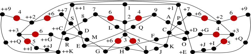
Figure 2. Bub’s MMP with 49 atoms and 36 blocks. Notice that 12 bigger dots with a pattern (red online) represent just 4 atoms: 4, 5, 6, and +6.

Bub’s set, shown in Fig. 2 is the smallest known KS setup.[5] Its MMP hypergraph reads: 123, 249, 267, 78++C, 9A+D, +1CK, ++1DE, 7LK, 9QE, 35I, 3+6G, EHI, IJK, +DFG, GM++C, CP+7, CO+G, ++1++C++K, ++3++2+1, +6++7++2, ++24++9, ++9++Q++K, ++35++I, ++I++J++K, ++36++G, ++GRD, DS++7, +3+2++1, +7+6+2, +26+9, +34+G, +35+I, +I+J+E, +1+D+E, +E+Q+9, 1+1++1. It is shown in Fig. 2

Peres’ set [6], shown in Fig. 3 is the most symmetric KS set among those with less than 60 vectors—it has 57 vectors (vertices) and 40 tetrads (edges). Its MMP hypergraph reads: 123, 345, 467, 789, 92A, ABC, CD4, AE+J, 5F+J, IG+9, IH+5, I7+1, JC++1, ++1+2+3, +3+4+5, +4+6+7, +7+8+9, +9+2+A, +A+B+C, +C+D+4, +A+E++J, +5+F++J, +I+G++9, +I+71, +I+H++5, +J+C+1, +1++2++3, ++3++4++5, ++4++6++7, ++7++8++9, ++9++2++A, ++A++B++C, ++C++D++4, ++A++EJ,++5++FJ, ++I++G9, ++I++7++1, ++I++H5, ++J++C1, 1+1++1. Another highly symmetrical KS set is the original Kochen-Specker’s one [23] but it contains 192 vectors.

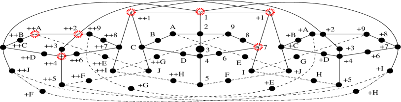
Figure 3. Peres’ KS MMP hypergraph/lattice. Red (online) rings denote atoms at which Peres’ lattice violates 7OA i.e. the failing assignment of atoms or co-atoms to the variables of 7OA in the form of Eq. (2.8).

Now, a number of authors have represented KS setups or indeed any spin-1 experimental setup by means of Greechie lattices.[24, 25, 26, 27, 28, 29, 30, 31, 32]

As we show above, the Hilbert lattice of any quantum system has to satisfy $n$OA equations. If we assume that the hypergraphs that describe Peres’ and Bub’s setups can be represented by lattices, we would end up with Greechie lattices for them, i.e., lattices that recognize only relations between orthogonal atoms and coatoms (spans) from such orthogonal sets. When we check—by our program latticeg described in Sec. 5—whether the Greechie lattices pass $n$OA equations, we find out that Bub’s lattice violates 3OA (and of course all $n$OA, $n>3$) and that Peres’ satisfies 3OA-6OA and violates 7OA. The reason that happens is simple: Greechie diagrams are not subalgebras of a Hilbert lattice and the aforementioned authors apparently did not realize that.

To convince ourselves that Peres’ and Bub’s Hilbert lattices really do satisfy 7OA and 8OA, it is enough to invoke Th. 2.8 according to which any quantum system (set of vectors/states ascribed to it) has to satisfy all $n$OA equations. But let us nevertheless go into some details with Bub’s Hilbert vectors so as to arrive at proper lattices and proper Hasse diagrams that they have to use. A proper description can only be carried out with lattices and Hasse diagrams that take into account joins (spans in terms of vectors) of nonorthogonal atoms (vectors) as well as the joins and meets (spans and intersections, respectively) of those joins, etc.

The details are as follows. We consider Bub’s KS setup. To be able to apply our program vectorfind for finding the vector components of Bub’s setup shown in Fig. 2, we have to write down its MMP representation without gaps in letters. So, we have 123,…,DFH,…, where we present only those Greechie/Hasse lattice atoms in which 3OA failed. Their Hilbert space vectors are: 1={0,0,1}, 2={1,0,0}, F={1,-2,-1}, and D={1,1,-1}.

In a Hilbert space representation, Bub’s KS setup does pass 3OA. Let us consider 3OA in the following form

$$a\perp b\quad\&\quad q\perp n\quad$$

$$\Rightarrow(a\cup b)\cap(q\cup n)\leq b\cup(a\cap(q\cup((a\cup q)\cap(b\cup n)))).$$

In 3-dim Euclidean space, all subspaces are closed (they are lines, planes, or the whole space), so $a\cup b=a+b$, i.e., subspace join and subspace sum are the same. Thus, converting joins in the previous equation to subspace sums and using the orthogonality we get:

$$a\perp b \quad\&\quad q\perp n\Rightarrow(a+b)\cap(q+n)$$

$$\leq b+(a\cap(q+((a+q)\cap(b+n)))).$$ (3.1)

Now, using the subspaces determined by the aforementioned vectors and their spans in a Hilbert space, we can easily check that Bub’s representation pass 3OA. For instance, vectors 1, 2, F, and D, determine subspaces {0,0,$\alpha$}, {$\beta$,0,0}, {$\gamma$,-2$\gamma$,-$\gamma$}, and {$\delta$,$\delta$,-$\delta$}, with arbitrary coefficients $\alpha,\dots$. They represent lines in both 3-dim Hilbert space and 3-dim Euclidean space. {0,0,$\alpha$}+{$\beta$,0,0}= {$\beta$,0,$\alpha$} is a plane spanned by 1 and 2, etc. We show a verification of Eq. (3.1) in Fig. 4.

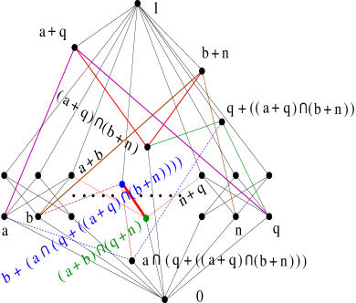
Figure 4. A new kind of lattice (MMPL) in which Bub’s setup passes 3OA. The inequality relation in Eq. (3.1) is represented by the thick line (red online).

Such lattices—we call them MMPLs—are essential for checking various other equations, because, e.g., the MMPL shown in Fig. 4 as an example of a lattice that satisfies 3OA for a particular nodal assignment to its variables, and we can further check whether it satisfies other equations that correspond to a particular experimental setup. Thus when we need a lattice to set up a blueprint for an experiment in which it is important that a system satisfy particular equations, we shall use MMPL. When we just need to find a lattice in which an equation fails and another pass to show their independence, a Greechie lattice might serve us better. Greechie lattices contain only relations between elements within orthogonal subsets of chosen lattices and therefore for more complicated equations soon become so large that one cannot compute them any more. Thus we were actually lucky to find that Peres’ lattice satisfied 6OA and violated 7OA because that provided an immediate proof that 7OA does not follow from 6OA.

4. Main Result: Lattices That Satisfy 6OA and Violate 7OA

Peres’ lattice violates 7OA at ++1, ++4, 1, 7, +1, ++A, ++23, and we have indicated these elements with the help of rings in Fig. 3. But rather than analyze the failure, we will show how we can arrive at a much smaller lattice that also satisfies 6OA and violates 7OA. The procedure shows how we can get smaller lattices using our program latticeg to eliminate atoms and blocks that did not take part in the violations of 7OA we originally found.

When we apply latticeg to the equation 7OA and it arrives at atoms (or more precisely, lattice nodes) at which 7AO fails, the program gives the nodes we listed above, and it also gives us the following additional information about the failure:

Greechie atoms not visited: 2 3 4 …

Greechie blocks that don’t affect the failure: 345 ABC CD4 …

If, during the evaluation of the failing assignment, the meets and joins contained in a block are never used, then that block is unrelated to the failure. The program accumulates such blocks and puts them into a list called “don’t affect the failure” as illustrated by the sample printout above. After removing these from the Peres’ Greechie lattice of Fig. 3 and renaming the atoms, we end up with the smaller Greechie lattice 123, 345, 567, 789, 9AB, BCD, DEF, FGH, HIJ, JKL, LMN, NOP, PQR, RS1, 4EK, 4AP, AVH, BXL, DUQ, FWN, JTQ   which is shown in Fig. 5. The left figure shows the blocks we dropped from Fig. 3, and the right one is given in the representation we previously used to show violations of 3OA through 6OA at lattices presented in [22, 9, 33] with the maximal loop (tetrakaidecagon, 14-gon) it contains.

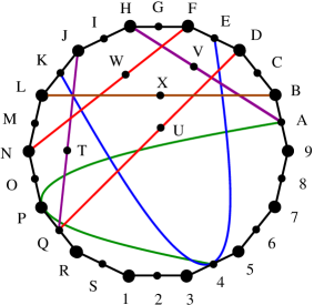
Figure 5. A lattice with 33 atoms and 21 blocks that satisfies 6OA and violates 7OA. Red (online) rings show atoms that take part in a violation of 7OA. The left and right diagrams are isomorphic to each other (i.e. are two ways of drawing the same lattice).

Of course, there is a whole series of lattices between Peres’ 57-40 and the 33-21 shown here with the same property of violating 7OA and satisfying 6OA which we obtain by adding the removed blocks to 33-21 lattice until we obtain Peres’.

The independence of 7OA emerged from our study to determine which quantum properties continue to hold when 3-dim KS setups are approximately (but erroneously, in a strict mathematical sense) represented by Greechie lattices. The passing of 6OA and failing of 7OA was fortuitous and quite unexpected. Previously, we had little hope of finding such an example with the help of Greechie diagrams. The discovery of a lattice passing 5OA but failing 6OA required many weeks on a 500-CPU cluster, and that discovery itself involved a large element of luck combined with some judicious intuition by the second author about which lattices might be promising. The search for a 7OA counterexample was expected to be many orders of magnitude harder. Even the verification that the single Peres’ lattice passed 6OA required weeks of cluster time, and had it not been for an early occurrence of a failure in the 7OA test, that test might have required a much longer time.

5. Algorithms and Programs

The main program that we used for this work was latticeg, which is a general-purpose utility for testing equations against orthocomplemented lattices expressed in the form of Greechie diagrams. Its algorithm is described in Ref. [34].

The $n$OA law in the form derived directly from Hilbert space, Eq. (2.6), has $2n-2$ variables, whereas in the equivalent form of Eq. (2.8) it has $n$ variables. Since testing an equation with $m$ variables against a lattice with $k$ nodes requires that up to $k^{m}$ combinations be checked, it is more efficient to use the form of Eq. (2.8).

Eq. (2.8) has $8\cdot 3^{n-3}+4$ occurrences of its $n$ variables. For faster computation, we found an equivalent with $6\cdot 3^{n-3}+3$ variable occurrences (which equals 166 for 6OA and 489 for 7OA). The following theorem shows this equivalent form for $n=3$. The proof is similar for larger $n$. The general form for larger $n$ can be inferred by looking at the proof, although we have not defined a “compact” notation for it as we have for Eq. (2.8).

Theorem 5.1.

An OML in which the equation

$$a\cap((a\cap b)\cup((a\to c)\cap(b\to c)))\leq b^{\prime}\to c$$ (5.1)

holds is a 3OA and vice-versa.

Proof.

For Eq. (5.1): To obtain the 3OA law, Eq. (2.8), from Eq. (5.1), we substitute $a\to c$ for $a$ and $b\to c$ for $b$, then we use the OML identities $(a\to c)\to c=a^{\prime}\to c$, $(b\to c)\to c=b^{\prime}\to c$, and $(b^{\prime}\to c)\to c=b\to c$.

For the converse, since $x\leq x^{\prime}\to y$,

$$a\cap(( a\cap b)\cup((a\to c)\cap(b\to c)))$$

$$\leq(a^{\prime}\to c)\cap(((a^{\prime}\to c)\cap(b^{\prime}\to c))\cup((a\to c)\cap(b\to c)))$$

$$=(a^{\prime}\to c)\cap(a^{\prime}{\buildrel c\over{\equiv}}b^{\prime})$$

$$\leq b^{\prime}\to c,$$

where for the last step we used an instance of Eq. (2.8) for $n=3$. ∎

Because of the large size of the $n$OA equations for larger $n$, in order to ensure that our input to latticeg was free from typos we used an auxiliary utility program, oagen, to generate $n$OA equations in the form of either Eq. (2.8) or Eq. (5.1).

The evaluation of the 7OA equation on the Peres Greechie diagram involves 7 nested loops, each with 116 iterations (since its Hasse diagram has 116 nodes). For the shorter equation of the form of Eq. (5.1), each evaluation at the innermost loop involves an assignment to 489 variable occurrences and 487 join, meet, and $\to$ operations (the last having a precomputed table in memory from its join, meet, and orthocomplementation expansion). Thus $116^{7}\cdot 489=138,202,145,015,414,784$ (138 quadrillion) operation evaluations ($489=487+1+1$ includes the final $\leq$ comparison and a single orthocomplementation) are required for a full scan.

Such a direct, full evaluation is a challenge on today’s hardware, even with a cluster of processors, unless one is very lucky to encounter a failure early on in the scan (and we were). In addition, we made several enhancements to latticeg to help make this project more feasible:

• The main algorithm was improved. The original algorithm assigned each possible combination of lattice nodes to the equation variables, then evaluated the resulting equation according to the structure of the lattice (i.e. the suprema, infima, and orthocomplements in the Hasse diagram derived from the input Greechie diagram). The main scan consists of nested loops that processes all nodal assignments to the first variable in the outermost loop, then all assignments to the second variable in the next inner loop, and so on. Since it has 7 variables, testing the 7OA equation involves 7 nested loops.

  The new algorithm takes into account, at each loop level, the variables in outer loops (which have known assignments) and evaluates as much of the equation as it can with those known variables. The equation is then shrunk with these partial evaluations, for further processing at that and deeper loop levels. Eventually, the equation is shrunk to a length of one, which means that it is completely evaluated. While a length of one will always be obtained at the innermost loop level, it may also occur at an outer level (such as when an expression containing not-yet-assigned variables is conjoined with a partial evaluation that resulted in lattice 0). In such cases, processing of further inner loops becomes unnecessary. So, the new algorithm benefits from (1) shorter equations to evaluate at deeper loop levels and (2) possible skipping of the deepest loops. Overall, this results in a speedup of about a factor of 10 for the 7OA equation evaluation.

  Because of the complexity of the new partial evaluation algorithm, it was put into a new version of latticeg called lattice2g. This allows us to check that the old and new algorithms produce the same result, helping to make sure there isn’t a program bug in the new algorithm. Having two programs also allows us to directly measure the speedup afforded by the new algorithm.

• For testing a huge lattice, a feature was added to break up the testing into several independent parts. This way the different parts can be run on different processors in our cluster. The test can be partitioned into any number of outermost and first inner loop iterations. For example, the Peres Greechie diagram has a Hasse representation with 116 nodes. We can specify that the cluster test the 98th iteration (out of 116) of the outmost loop and the 101st through 110th iteration (out of 116) of the next inner loop.

• A feature was added to analyze an equation failure to determine what nodes, atoms, and blocks were not involved in the failure. In particular, a block is said not to affect the failure whenever all operations that “visit” (non-0 and non-1) nodes in the block do not involve any other (non-0 and non-1) nodes in that block. This is described in more detail in Sec. 4, where we show how this feature was used to determine which blocks could be removed from Peres’ Greechie lattice to obtain a smaller lattice that satisfies 6OA but violates 7OA

6. Conclusion

After 75 years of research carried out in the field of the algebraic structure underlying quantum Hilbert space—the Hilbert lattice—only one class of equations (beyond the orthomodular lattice laws) that hold in it was found: the class of orthoarguesian equations. Individual orthoarguesian equations were found in the eighties and nineties. All other equations known to hold in a Hilbert lattice require a state introduced to it.

Then in 2000 we found [8] a class ($n$oa) of lattices determined by generalized orthoarguesian equations ($n$OA) and proved that the following inclusion holds: $n{\rm oa}\subseteq(n+1){\rm oa}$. We also proved that all previously found OAs are equivalent to either 3OA or 4OA, we proved that 4OA is strictly stronger than 3OA, and we found lattices in which 4OA passed but 5OA failed and lattices in which 5OA passed and 6OA failed. [9]

In this paper we found a series of lattices—shown in Figs. 3 and 5 and obtained as explained in Sec. 4—in which 6OA passes and 7OA fails. This is important because it very strongly indicates that the above inclusion is strict: $n{\rm oa}\subset(n+1){\rm oa}$.

We obtained these lattices by analyzing Kochen-Specker sets. The Kochen-Specker sets correspond to strictly quantum systems. They cannot be given a classical interpretation at all, and therefore their lattice representation should be a proper lattice representation. We wanted to find out how they can be constructed, what they look like, and what their Hasse diagrams look like. In the literature, we only found that 3-dim KS systems in particular and spin-1 systems in general were described by Greechie diagrams (as we stressed in the Introduction).

To our surprise, all but Peres’ Greechie lattices violated 3OA, and to our joy Peres’ Greechie lattice passed 3OA through 6OA but violated 7OA. We say surprise, because every lattice of a quantum system must be represented by a sublattice of a Hilbert lattice, and the violations of OAs meant that the representation by Greechie lattices is incorrect. It is incorrect because the Greechie lattices are not sublattices of the lattice of closed subspaces of a Hilbert space, a fact that escaped the authors mentioned in the Introduction. Therefore in Sec. 3, we explain what a proper lattice of any quantum system should look like and how we can use MMPLs when we need a lattice for a particular system which passes particular equations.

We should mention out that the numbers of elements (atoms and blocks) of the smallest known lattices that satisfy $n$OA but violate $(n+1)$OA do not grow exponentially. For $3\leq n\leq 7$ we have 13, 17, 22, 28, 33 and 7, 10, 13, 18, 21 atoms and blocks, respectively. [9] An important open question is whether there is a pattern that can be identified in this or a similar series of lattices. If so, that might lead to a proof that $(n+1)$OA is strictly stronger than $n$OA for all $n$.

Since the class of Hilbert lattices (HL) is a subclass of $n$oa for all $n$ (as Th. 2.6 shows), an open question is what additional conditions must be added to $n$OA to specify HL, for both the finite and infinite dimensional cases? Are there other classes of equations that hold in every HL when we do not introduce states on it? (The other known equations such as Godowski’s and Mayet’s [9] assume states.) How far can we define HL only by means of sets of equations added to an OL?

Acknowledgment

One of us (M. P.) would like to thank his host Hossein Sadeghpour for support during his stay at ITAMP.

Supported by the US National Science Foundation through a grant for the Institute for Theoretical Atomic, Molecular, and Optical Physics (ITAMP) at Harvard University and Smithsonian Astrophysical Observatory and the Ministry of Science, Education, and Sport of Croatia through the project No. 082-0982562-3160.

Computational support was provided by the cluster Isabella of the University Computing Centre of the University of Zagreb and by the Croatian National Grid Infrastructure.

References

- [1] G. Birkhoff and J. von Neumann, The Logic of Quantum Mechanics, Ann. Math. 37, 823–843 (1936).
- [2] E. G. Beltrametti and G. Cassinelli, The Logic of Quantum Mechanics, Addison-Wesley, 1981.
- [3] S. S. Holland, Jr., Orthomodularity in Infinite Dimensions; a Theorem of M. Solèr, Bull. Am. Math. Soc. 32, 205–234 (1995).
- [4] M. Pavičić, B. D. McKay, N. D. Megill, and K. Fresl, Graph Approach to Quantum Systems, ArXiv:1004.0776 2010 .
- [5] J. Bub, Schütte’s Tautology and the Kochen–Specker Theorem, Found. Phys. 26, 787–806 (1996).
- [6] A. Peres, Two Simple Proofs of the Bell–Kochen–Specker Theorem, J. Phys. A 24, L175–L178 (1991).
- [7] M. Pavičić, J.-P. Merlet, and N. D. Megill, Exhaustive Enumeration of Kochen–Specker Vector Systems, The French National Institute for Research in Computer Science and Control Research Reports RR-5388 (2004).
- [8] N. D. Megill and M. Pavičić, Equations, States, and Lattices of Infinite-Dimensional Hilbert Space, Int. J. Theor. Phys. 39, 2337–2379 (2000).
- [9] M. Pavičić and N. D. Megill, Quantum Logic and Quantum Computation, in Handbook of Quantum Logic and Quantum Structures, edited by K. Engesser, D. Gabbay, and D. Lehmann, volume Quantum Structures, pages 751–787, Elsevier, Amsterdam, 2007.
- [10] C. J. Isham, Lectures on Quantum Theory, Imperial College Press, London, 1995.
- [11] P. R. Halmos, Introduction to Hilbert Space and the Spectral Theory of Spectral Multiplicity, Chelsea, New York, 1957.
- [12] G. Kalmbach, Orthomodular Lattices, Academic Press, London, 1983.
- [13] P. Mittelstaedt, Quantum Logic, Synthese Library; Vol. 126, Reidel, London, 1978.
- [14] L. Beran, Orthomodular Lattices; Algebraic Approach, D. Reidel, Dordrecht, 1985.
- [15] M. Pavičić and N. D. Megill, Is Quantum Logic a Logic?, in Handbook of Quantum Logic and Quantum Structures, edited by K. Engesser, D. Gabbay, and D. Lehmann, volume Quantum Logic, pages 23–47, Elsevier, Amsterdam, 2009.
- [16] G. Birkhoff, Lattice Theory, volume XXV of American Mathematical Society Colloqium Publications, American Mathematical Society, New York, 2nd (revised) edition, 1948.
- [17] G. Birkhoff, Lattice Theory, volume XXV of American Mathematical Society Colloquium Publications, American Mathematical Society, Providence, Rhode Island, 3rd (new) edition, 1967.
- [18] M. Pavičić, Nonordered Quantum Logic and Its YES–NO Representation, Int. J. Theor. Phys. 32, 1481–1505 (1993).
- [19] M. Pavičić, Identity Rule for Classical and Quantum Theories, Int. J. Theor. Phys. 37, 2099–2103 (1998).
- [20] G. Kalmbach, Measures and Hilbert Lattices, World Scientific, Singapore, 1986.
- [21] P.-A. Ivert and T. Sjödin, On the Impossibility of a Finite Propositional Lattice for Quantum Mechanics, Helv. Phys. Acta 51, 635–636 (1978).
- [22] N. D. Megill and M. Pavičić, Equations, States, and Lattices of Infinite-Dimensional Hilbert Space, Int. J. Theor. Phys. 39, 2337–2379 (2000), ArXiv/quant-ph/0009038.
- [23] S. Kochen and E. P. Specker, The problem of hidden variables in quantum mechanics, J. Math. Mech. 17, 59–87 (1967).
- [24] B. O. Hultgren, III and A. Shimony, The Lattice of Verifiable Propositions of the Spin-1 System, J. Math. Phys. 18, 381–394 (1977).
- [25] B. O. Hultgren, III, A Lattice of Verifiable Propositions, PhD thesis, Boston University Graduate School, 1974.
- [26] K. Svozil and J. Tkadlec, Greechie Diagrams, Nonexistence of Measures and Kochen–Specker-Type Constructions, J. Math. Phys. 37, 5380–5401 (1996).
- [27] K. Svozil, Quantum Logic, Discrete Mathematics and Theoretical Computer Science, Springer-Verlag, New York, 1998.
- [28] J. Tkadlec, Greechie Diagrams of Small Quantum Logics with Small State Spaces, Int. J. Theor. Phys. 37, 203–209 (1998).
- [29] J. Tkadlec, Diagrams of Kochen–Specker Constructions, Int. J. Theor. Phys. 39, 921–926 (2000).
- [30] J. Tkadlec, Representations of Orthomodular Structures, in Ordered Algebraic Structures: Nanjing; Proceedings of the Nanjing Conference, edited by W. C. Holland, volume 16 of Algebra, Logic and Applications, pages 153–158, London, 2001, Taylor & Francis.
- [31] D. Smith, Algebraic Partial Boolean Algebras, J. Phys. A 36, 3899–3910 (2003).
- [32] D. J. Foulis, A Half-Century of Quantum Logic—What Have We Learned?, in Quantum Structures and the Nature of Reality, edited by D. Aerts and J. Pykacz, Proceedings of the Conference: The Indigo Book of Einstein Meets Magritte, pages 1–36, Dordrecht, 1999, Kluwer Academic Publishers.
- [33] N. D. Megill and M. Pavičić, Hilbert Lattice Equations, Ann. Henri Poincaré 10, 1335–1358 (2010).
- [34] B. D. McKay, N. D. Megill, and M. Pavičić, Algorithms for Greechie Diagrams, Int. J. Theor. Phys. 39, 2381–2406 (2000), ArXiv/quant-ph/0009039.