Orbits Around Black Holes in Triaxial Nuclei

Abstract

We discuss the properties of orbits within the influence sphere of a supermassive black hole (BH), in the case that the surrounding star cluster is nonaxisymmetric. There are four major orbit families; one of these, the pyramid orbits, have the interesting property that they can approach arbitrarily closely to the BH. We derive the orbit-averaged equations of motion and show that in the limit of weak triaxiality, the pyramid orbits are integrable: the motion consists of a two-dimensional libration of the major axis of the orbit about the short axis of the triaxial figure, with eccentricity varying as a function of the two orientation angles, and reaching unity at the corners. Because pyramid orbits occupy the lowest angular momentum regions of phase space, they compete with collisional loss cone repopulation and with resonant relaxation in supplying matter to BHs. General relativistic advance of the periapse dominates the precession for sufficiently eccentric orbits, and we show that relativity imposes an upper limit to the eccentricity: roughly the value at which the relativistic precession time is equal to the time for torques to change the angular momentum. We argue that this upper limit to the eccentricity should apply also to evolution driven by resonant relaxation, with potentially important consequences for the rate of extreme-mass-ratio inspirals in low-luminosity galaxies. In giant galaxies, we show that capture of stars on pyramid orbits can dominate the feeding of BHs, at least until such a time as the pyramid orbits are depleted; however this time can be of order a Hubble time.

1. Introduction

Following the demonstration that self-consistent equilibria could be constructed for triaxial galaxy models (Schwarzschild, 1979, 1982), observational evidence gradually accumulated for non-axisymmetry on large (kiloparsec) scales in early-type galaxies (Franx et al., 1991; Statler et al., 2004; Cappellari et al., 2007). On smaller scales, imaging of the centers of galaxies also revealed a wealth of features in the stellar distribution that are not consistent with axisymmetry, including bars, bars-within-bars, and nuclear spirals (Shaw et al., 1993; Erwin & Sparke, 2002; Seth et al., 2008). In the nuclei of low-luminosity galaxies, the non-axisymmetric features may be recent or recurring, associated with ongoing star formation; in luminous elliptical galaxies, central relaxation times are so long that triaxiality, once present, could persist for the age of the universe.

In a triaxial nucleus, torques from the stellar potential can induce gradual changes in the eccentricities of stellar orbits, allowing stars to find their way into the central BH. Gravitational two-body scattering also drives stars into the central BH, but only on a time scale of order the central relaxation time, which can be very long, particularly in the most luminous galaxies. Simple arguments suggest that the feeding of stars to the central BHs in many galaxies is likely to be dominated by large-scale torques rather than by two-body relaxation (e.g. Merritt & Poon, 2004).

This paper discusses the character of orbits near a supermassive BH in a triaxial nucleus. The emphasis is on low-angular-momentum, or “centrophilic,” orbits, the orbits that come closest to the BH. Self-consistent modelling (Poon & Merritt, 2004) reveals that a large fraction of the orbits in triaxial BH nuclei can be centrophilic.

Within the BH influence sphere, orbits are nearly Keplerian, and the force from the distributed mass can be treated as a small perturbation which causes the orbital elements (inclination, eccentricity) to change gradually with time. A standard way to deal with such motion is via orbit averaging (e.g. Sanders & Verhulst, 1985), i.e., averaging the equations of motion over the short time scale associated with the unperturbed Keplerian motion. The result is a set of equations describing the slow evolution of the remaining orbital elements due to the perturbing forces. This approach was followed by Sridhar & Touma (1999) for motion in an axially-symmetric nucleus containing a massive BH, and by Sambhus & Sridhar (2000) for motion in a constant-density triaxial nucleus.

In their discussion of motion in triaxial nuclei, Sambhus & Sridhar (2000) passed over one important class of orbit: the centrophilic orbits, i.e., orbits that pass arbitrarily close to the BH. Examples of centrophiliic orbits include the two-dimensional “lens” orbits (Sridhar & Touma, 1997, 1999) and the three-dimensional “pyramids” (Merritt & Valluri, 1999; Poon & Merritt, 2001). Centrophilic orbits are expected to dominate the supply of stars and stellar remnants to a supermassive BH (e.g. Merritt & Poon, 2004) and are the focus of the current paper.

The paper is organized as follows. In §2 we present a model for the gravitational potential of a triaxial nuclear star cluster, which is more general than that studied in Sambhus & Sridhar (2000), but which has many of the same dynamical features. Then in §3 we write down the orbit-averaged equations of motion, and in §4 present a detailed analytical study of their solutions, with emphasis on the case where the triaxiality is weak and the eccentricity large. In this limiting case, the averaged equations of motion turn out to be fully integrable. In §5 we derive the equations that describe the rate of capture of stars on pyramid orbits by the BH. Comparison of orbit-averaged treatment with real-space motion is made in §6, to test the applicability of the former. In §7 we consider the effect of general relativity on the motion, which imposes an effective upper limit on the eccentricty. §8 discusses the connection with resonant relaxation: we argue that a similar upper limit to the eccentricity should characterize orbital evolution in the case of resonant relaxation. Finally, in §9 we make some quantitative estimates of the importance of pyramid orbits for capture of stars in galactic nuclei. §10 sums up.

2. Model for the nuclear star cluster

Consider a nucleus consisting of a BH, a spherical star cluster, and an additional triaxial component. An expression for the gravitational potential that includes the three components is

$$\Phi({\bf r}) = -\frac{G{M_{\bullet}}}{r}+\Phi_{s}\left(\frac{r}{r_{0}}\right)^{2-\gamma}$$

$$+ 2\pi\,G\rho_{t}\,\left(T_{x}x^{2}+T_{y}y^{2}+T_{z}z^{2}\right).$$

The second term on the right hand side is the potential of a spherical star cluster with density $\rho(r)=\rho_{s}(r/r_{0})^{-\gamma}$; the coefficient $\Phi_{s}$ is given by

$$\Phi_{s}=\frac{4\pi G}{(3-\gamma)(2-\gamma)}\rho_{s}r_{0}^{2}.$$

The scale radius $r_{0}$ may be chosen arbitrarily but it is convenient to set $r_{0}=r_{\mathrm{infl}}$, with $r_{\mathrm{infl}}$ the radius at which the enclosed stellar mass is twice ${M_{\bullet}}$:

$$r_{\mathrm{infl}}=\left(\frac{3-\gamma}{2\pi}\frac{{M_{\bullet}}}{\rho_{s}}\right)^{1/3}.$$ (2)

The third term is the potential of a homogeneous triaxial ellipsoid of density $\rho_{t}$; this term can also be interpreted as a first approximation to the potential of a more general, inhomogeneous triaxial component. In the former case, the dimensionless coefficients ($T_{x},T_{y},T_{z}$) are expressible in terms of the axis ratios $(p,q)$ of the ellipsoid via elliptic integrals (Chandrasekhar, 1969). The $x(z)$ axes are assumed to be the long(short) axes of the triaxial figure; this implies $T_{x}\leq T_{y}\leq T_{z}$. In what follows we will generally assume $\rho_{t}\ll\rho_{s}(r_{0})$, i.e. that the triaxial bulge has a low density compared with that of the spherical cusp at $r=r_{\mathrm{infl}}$.

3. Orbit-averaged equations

Within the BH influence sphere, orbits are nearly Keplerian and the force from the distributed mass can be treated as a small perturbation which causes the elements of the orbit (inclination, eccentricity etc.) to change gradually with time. A standard way to deal with such motion (e.g. Sanders & Verhulst, 1985) is to average the equations over the coordinate executing the most rapid variation, e.g., the radius. The result is a set of equations describing the slow evolution of the remaining variables due to the perturbing forces.

We begin by transforming from Cartesian coordinates to action-angle variables in the Kepler problem. Following Sridhar & Touma (1999) and Sambhus & Sridhar (2000), we adopt the Delaunay variables (e.g. Goldstein et al., 2002) to describe the unperturbed motion.

Let $a$ be the semi-major axis of the Keplerian orbit. The Delaunay action variables are the radial action $I=(G{M_{\bullet}}a)^{1/2}$, the angular momentum $L$, and the projection of $\mathbf{L}$ onto the $z$ axis $L_{z}$. The conjugate angle variables are the mean anomaly $w$, the argument of the periapse $\varpi$, and the longitude of the ascending node $\Omega$. In the Keplerian case, five of these are constants; the exception is $w$ which increases linearly with time at a rate

$$\nu_{r}=(GM_{\bullet})^{2}/I^{3}$$ (3)

In terms of the new variables, the Hamiltonian is

$${\cal H}=-\frac{1}{2}\left(\frac{GM_{\bullet}}{I}\right)^{2}+\Phi_{p}(I,L,L_{z},w,\varpi,\Omega);$$ (4)

the first term is the Keplerian contribution and $\Phi_{p}$, the “perturbing potential”, contains the contributions from the spherical and triaxial components of the distributed mass. This transformation is completely general if we interpret the new variables as instantaneous (osculating) orbital elements. However if we assume that the perturbing potential is small compared with the point-mass potential, the rates of change of these variables (again with the exception of $w$) will be small compared with the radial frequency $\nu_{r}$, and the new variables can be regarded as approximate orbital elements that change little over a radial period $P\equiv 2\pi/\nu_{r}$. Accordingly, we average the Hamiltonian over the fast angle $w$:

$$\overline{\cal H} = -\frac{1}{2}\left(\frac{GM_{\bullet}}{I}\right)^{2}+\overline{\Phi}_{p},$$ (5a)

$$\overline{\Phi}_{p} \equiv \oint\frac{dw}{2\pi}\Phi=\frac{1}{2\pi}\int_{0}^{2\pi}dE\,(1-e\cos E)\,\Phi_{p}({\bf r}).$$ (5b)

The final term replaces the mean anomaly $w$ by the eccentric anomaly $E$, where $r=a(1-e\cos E)$ and the eccentricity is $e=\sqrt{1-L^{2}/I^{2}}$. After the averaging, $\overline{\cal H}$ is independent of $w$, and $I$ is conserved, as is the semi-major axis $a$. We are left with four variables and with $\overline{\Phi}_{p}$ as the effective Hamiltonian of the system.

The spherically symmetric part of $\overline{\Phi}_{p}$ is

$$\overline{\Phi}_{s} = F_{\gamma}(e)\,\Phi_{s}\left(\frac{a}{r_{0}}\right)^{2-\gamma},$$ (6)

$$F_{\gamma}(e) \equiv {}_{2}F_{1}\left(\left[-\frac{3-\gamma}{2},-\frac{2-\gamma}{2}\right],[1],e^{2}\right).$$

A good approximation to $F_{\gamma}(e)$ is

$$F_{\gamma}(e)\approx 1+\alpha e^{2}\;,\quad\alpha=\frac{2^{3-\gamma}\Gamma(\frac{7}{2}-\gamma)}{\sqrt{\pi}\,\Gamma(4-\gamma)}-1$$ (7)

which is exact for $\gamma=0$ and $\gamma=1$; for $0\leq\gamma<2$, $0<\alpha\leq 3/2$. When $\gamma>1$ and $e$ is close to 1, a better approximation is

$$F_{\gamma}(e)\approx 1+\alpha+\alpha^{\prime}(e^{2}-1)\;,\quad\alpha^{\prime}=\frac{2^{1-\gamma}(2-\gamma)}{\sqrt{\pi}}\frac{\Gamma(\frac{5}{2}-\gamma)}{\Gamma(3-\gamma)}.$$ (8)

We adopt the latter expression in what follows. Good approximations are

$$\alpha \approx \textstyle\frac{3}{2}-\frac{79}{60}\gamma+\frac{7}{20}\gamma^{2}-\frac{1}{30}\gamma^{3},$$ (9a)

$$\alpha^{\prime} \approx \textstyle\frac{3}{2}-\frac{29}{20}\gamma+\frac{11}{20}\gamma^{2}-\frac{1}{10}\gamma^{3}.$$ (9b)

Similar expressions can be found in Ivanov, Polnarev & Saha (2005) and Polyachenko, Polyachenko & Shukhman (2007).

Expressions for the orbit-averaged triaxial harmonic potential (excluding the spherical component) are derived in Sambhus & Sridhar (2000). Adopting their notation, the orbit-averaged potential in our case becomes

$$\overline{\Phi}_{p} = \Phi_{s}\left(\frac{a}{r_{0}}\right)^{2-\gamma}(1+\alpha-\alpha^{\prime}\ell^{2})+2\pi G\rho_{t}T_{x}\,a^{2}\times$$

$$\times \left[\frac{5}{2}-\frac{3}{2}\ell^{2}+\epsilon_{b}^{(t)}H_{b}(\ell,\ell_{z},\varpi,\Omega)+\epsilon_{c}^{(t)}H_{c}(\ell,\ell_{z},\varpi)\right]$$

$$H_{b} = {\textstyle\frac{1}{2}}\left[(5-4\ell^{2})(c_{\varpi}s_{\Omega}+c_{i}c_{\Omega}s_{\varpi})^{2}\right.$$

$$+ \left.\ell^{2}(s_{\varpi}s_{\Omega}-c_{i}c_{\Omega}c_{\varpi})^{2}\right],$$

$$H_{c} = {\textstyle\frac{1}{4}}(1-c_{i}^{2})[5-3\ell^{2}-5(1-\ell^{2})c_{2\varpi}],$$ (10c)

$$\epsilon_{b}^{(t)} \equiv T_{y}/T_{x}-1\;,\quad\epsilon_{c}^{(t)}\;\equiv\;T_{z}/T_{x}-1.$$ (10d)

The shorthand $s_{x},c_{x}$ has been used for $\sin x,\cos x$. We have defined the dimensionless variables $\ell=L/I$ and $\ell_{z}=L_{z}/I$, both of which vary from 0 to 1; the orbital inclination $i$ is given by $\cos i\equiv\ell_{z}/\ell$ and the eccentricity by $e^{2}=1-\ell^{2}$.

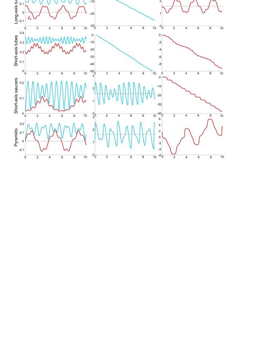
Figure 1.— Four classes of orbits around a BH in a triaxial nucleus. Left column: time dependence of the dimensionless angular momentum $\ell$ (top/blue) and its component $\ell_{z}$ along the short axis of the figure (bottom/red). Middle column: argument of the periapse $\varpi$. Right column: angle of nodes $\Omega$.

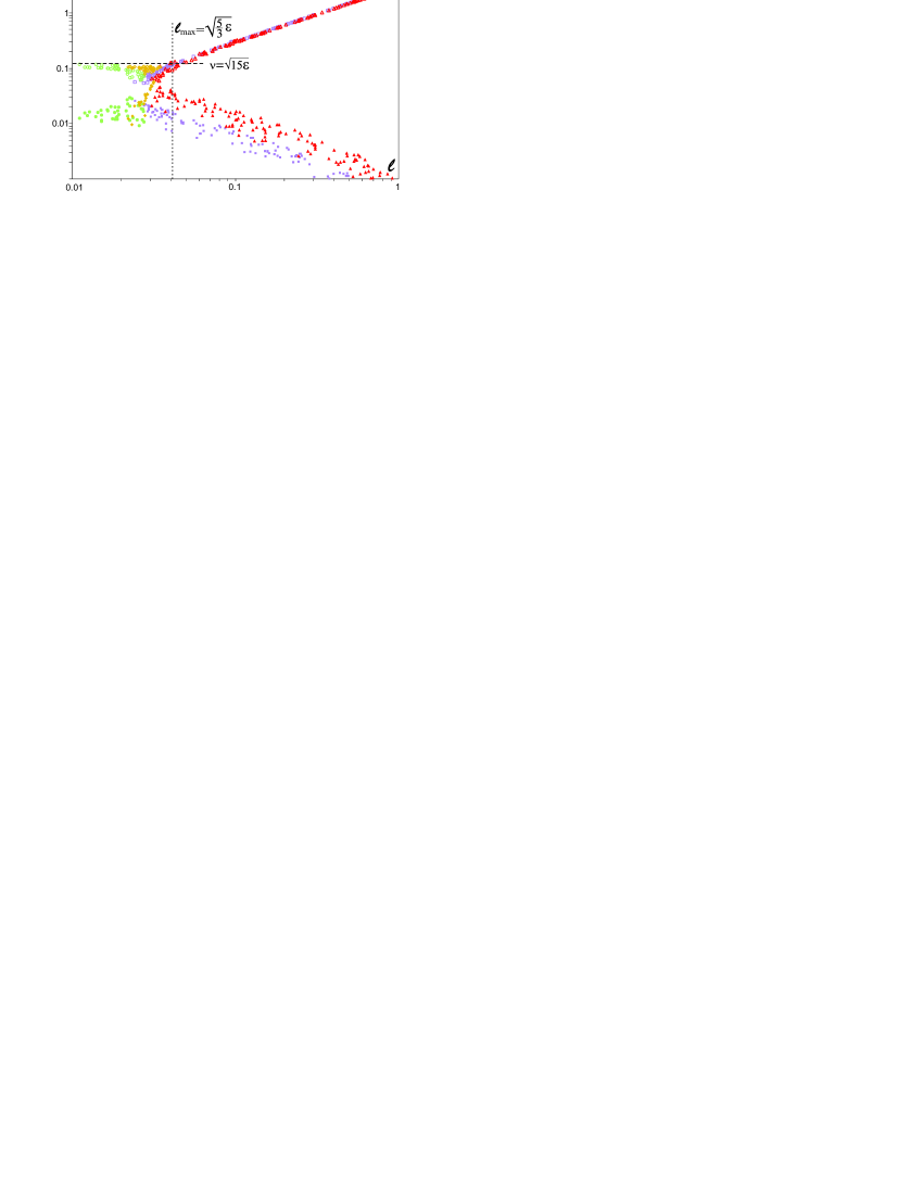
Figure 2.— Dependence of the characteristic frequencies $\nu_{\varpi}$ (in-plane precession) and $\nu_{\Omega}$ (nodal precession) on the value of the dimensionless angular momentum $\ell$. Top (open) symbols: $\nu_{\varpi}$; bottom (filled) symbols: $\nu_{\Omega}$. Magenta boxes: LATs; red triangles: SATs; yellow diamonds: saucers; green circles: pyramids. For large $\ell$ $\nu_{\varpi}\propto\ell$ and $\nu_{\Omega}\ll\nu_{\varpi}$, but for sufficiently low $\ell$ these two are comparable, which gives birth to the pyramid and saucer orbits. Vertical line denotes the threshold in $\ell$ (equation 36), horizontal line the characteristic frequency $\nu_{x0}$ (equation 22). Triaxiality coefficients were set to $\epsilon_{c}=10^{-3}$, $\epsilon_{b}=0.4\epsilon_{c}$.

The first term in equation (10), which arises from the spherically-symmetric cusp, does not depend on the angular variables, and has the same dependence on $\ell^{2}$ as the corresponding term in the harmonic triaxial potential. So we can sum up the coefficients at $\ell^{2}$ and renormalize the triaxial coefficients $\epsilon_{b,c}$ to obtain the same functional form of the Hamiltonian as in the purely harmonic case. Dropping an unnecessary constant term (depending only on $a$) and defining a dimensionless time $\tau=\nu_{p}t$, where $\nu_{p}$ is characteristic rate of precession,

$$\nu_{p} \equiv 2\pi G\rho_{t}T_{x}a^{2}(1+A)/I\;,$$ (11)

$$A \equiv {\textstyle\frac{4\alpha^{\prime}}{3(3-\gamma)(2-\gamma)T_{x}}}\frac{\rho_{s}}{\rho_{t}}\left(\frac{a}{r_{0}}\right)^{-\gamma},$$ (12)

we obtain the dimensionless Hamiltonian and the equations of motion describing the perturbed motion:

$$H \equiv \frac{\overline{\Phi}_{p}}{\nu_{p}I}=-\frac{3}{2}\ell^{2}+\epsilon_{b}H_{b}+\epsilon_{c}H_{c},$$ (13a)

$$\frac{d\ell}{d\tau} = -\frac{\partial H}{\partial\varpi},\ \frac{d\varpi}{d\tau}=\frac{\partial H}{\partial\ell},\ \frac{d\ell_{z}}{d\tau}=-\frac{\partial H}{\partial\Omega},\ \frac{d\Omega}{d\tau}=\frac{\partial H}{\partial\ell_{z}}.\qquad\mathstrut$$ (13b)

The renormalized triaxiality coefficients are $\epsilon_{b,c}\equiv\epsilon_{b,c}^{(t)}/(1+A)$.

If there were no spherical component ($A=0$), this would reduce to the purely harmonic triaxial case studied by Sambhus & Sridhar (2000). Adding the spherically symmetric cusp increases the rate of periapse precession, while at the same time reducing the relative amplitude of the triaxial terms; otherwise the form of the Hamiltonian is essentially unchanged.

A more transparent expression for the precession frequency $\nu_{p}$ is

$$\nu_{p} = \nu_{r}\left(\frac{M_{t}(a)}{M_{\bullet}}\frac{3T_{x}}{2}+\frac{M_{s}(a)}{M_{\bullet}}\frac{2\alpha^{\prime}}{3(2-\gamma)}\right)$$ (14a)

$$M_{t}(a) \equiv \frac{4\pi}{3}a^{3}\rho_{t}\;\;,\quad M_{s}(a)\equiv\frac{4\pi}{3-\gamma}a^{3}\rho_{s}\left(\frac{a}{r_{0}}\right)^{-\gamma}$$ (14b)

where $M(a)$ denotes the mass enclosed within radius $r=a$. From equation (13b), the precession rate of an orbit in the spherical cluster is $\nu_{\varpi}\equiv|d\varpi/dt|=3\ell\nu_{p}=3\sqrt{1-e^{2}}\,\nu_{p}$. Near the BH influence radius, it is clear that $\nu_{p}\approx\nu_{r}$; hence the orbit-averaged treatment, which assumes only one “fast” variable, is likely to break down at this radius.

We note that $\nu_{\varpi}\rightarrow 0$ as $e\rightarrow 1$. For the very eccentric orbits that are the focus of this paper, the rate of precession is much lower than for a typical, non-eccentric orbit of the same energy. This will turn out to be important, since the slow precession allows torques from the triaxial part of the potential to build up.

4. Orbital structure of the model potential

4.1. General remarks

The orbit-averaged Hamiltonian (13a) describes a dynamical system of two degrees of freedom. The trajectories must be obtained by numerical integration of the equations of motion (13b). We begin by making some qualitative points about the nature of the solutions.

In the absence of the triaxial terms in equation (13a), the effect of the distributed mass is to rotate the periapse angle $\varpi$ in a fixed plane; this steadily rotating elliptic orbit fills an annulus. The addition of a weak triaxial perturbation changes the rate of in-plane precession slightly, and also causes the orbital plane itself to change, as described by the last two terms in equation (13b).

In general, two angular variables $\varpi$ and $\Omega$ can either librate around fixed points or circulate, giving rise to four basic families of orbits (Figure 1). Solutions to the equations of motion that are characterized by circulation in both $\varpi$ and $\Omega$ correspond to tube orbits about the short axis (SAT). Motion that circulates in $\varpi$ but librates in $\Omega$ corresponds to tube orbits about the long axis (LAT). Both types of orbit are qualitatively similar to the tube orbits that are generic to the triaxial geometry (Schwarzschild, 1979). A subclass of the SAT orbits corresponds to motion that circulates in $\Omega$ and librates in $\varpi$ (Sambhus & Sridhar, 2000; Poon & Merritt, 2001). These orbits resemble cones, or saucers; similar orbits exist also at $r\gg r_{\mathrm{infl}}$ in oblate or nearly oblate potentials (Richstone, 1982; Lees & Schwarzschild, 1992).

If the degree of triaxiality is small ($\epsilon_{b,c}\ll 1$), then as noted above, the dominant effect of the distributed mass is simply to induce a periapse shift, at a rate $\nu_{\varpi}\equiv d\varpi/d\tau=-3\ell$. If the additional mass is much less than the mass of the BH, then on short time scales (comparable to the radial period $\nu_{r}^{-1}$) the orbit resembles a nearly closed ellipse. On intermediate time scales (of order the precession time $\nu_{\varpi}^{-1}$), a steadily-rotating elliptic orbit fills an annulus in a fixed plane. On still longer time scales $\nu_{\Omega}^{-1}$, the orbital plane itself changes due to the torques from the triaxial potential. Similar considerations give rise to the concept of vector resonant relaxation (Rauch & Tremaine, 1996).

The foregoing description is valid as long as the angular momentum is not too low. Since the precession rate is proportional to $\ell$, for sufficiently low $\ell$ the intermediate and long time scales become comparable (Figure 2). As a result, the triaxial torques can produce substantial changes in $\ell$ (i.e. the eccentricity) on a precession time scale via the first term in (13b), and the circulation in $\varpi$ can change to libration. This is the origin of the pyramid orbits, which are unique to the triaxial geometry (Merritt & Valluri, 1999).

4.2. Pyramid orbits

Of the four orbit families discussed above, the first three were treated, in the orbit-averaged approximation, by Sambhus & Sridhar (2000). The fourth class of orbits, the pyramids, are three-dimensional analogs of the two-dimensional “lens” orbits discussed by Sridhar & Touma (1997), also in the context of the orbit-averaged equations. An important property of the pyramid orbits is that $\ell$ can come arbitrarily close to zero (Poon & Merritt, 2001) and Merritt & Poon (2004). This makes the pyramids natural candidates for providing matter to BHs at the centers of galaxies.

Pyramid orbits can be treated analytically if the following two additional aproximations are made: (1) the angular momentum is assumed to be small, $\ell^{2}\ll 1$; (2) the triaxial component of the potential is assumed to be small compared with the spherical component, i.e. $\epsilon_{b},\epsilon_{c}\ll 1$. As shown below, these two conditions are consistent, in the sense that $\ell_{\mathrm{max}}^{2}\sim\epsilon_{b,c}$ for pyramid orbits.

Removing the second-order terms in $\epsilon_{b},\epsilon_{c}$ and in $\ell^{2}$ from the orbit-averaged Hamiltonian (13a), we find

$$H=-\frac{3}{2}\ell^{2}+\frac{5}{2}\left[\epsilon_{c}(1-c_{i}^{2})s_{\varpi}^{2}+\epsilon_{b}(c_{\varpi}s_{\Omega}+c_{i}s_{\varpi}c_{\Omega})^{2}\right]$$ (15)

where again $c_{i}\equiv\cos i=\ell_{z}/\ell$.

Because an orbit described by (15) is essentially a precessing rod, one expects the important variables to be the two that describe the orientation of the rod, and its eccentricity. This argument led us to search for exact solutions to the equations of motion in terms of the Laplace-Runge-Lenz vector, or its dimensionless counterpart, the eccentricity vector, which point in the direction of orbital periapse.

We therefore introduced new variables $e_{x}$, $e_{y}$ and $e_{z}$:

$$e_{x} = \cos\varpi\,\cos\Omega-\sin\varpi\,\cos i\,\sin\Omega$$ (16a)

$$e_{y} = \sin\varpi\,\cos i\,\cos\Omega+\cos\varpi\,\sin\Omega$$ (16b)

$$e_{z} = \sin\varpi\,\sin i$$ (16c)

which correspond to components of a unit vector in the direction of the eccentricity vector. Of these, only two are independent, since $e_{x}^{2}+e_{y}^{2}+e_{z}^{2}=1$. In terms of these variables, the Hamiltonian (15) takes on a particularly simple form:

$$H=-\frac{3}{2}\ell^{2}+\frac{5}{2}\left[\epsilon_{c}-\epsilon_{c}e_{x}^{2}-(\epsilon_{c}-\epsilon_{b})e_{y}^{2}\right].$$ (17)

As expected, the Hamiltonian depends on only three variables: $e_{x}$ and $e_{y}$, which describe the orientation of the orbit’s major axis, and the eccentricity $\ell$.

To find the equations of motion, we must switch to a Lagrangian formalism. Taking the first time derivatives of equations (16) and using equations (13b), we find

$$\dot{e}_{x}=3\ell(\sin\varpi\,\cos\Omega+\cos\varpi\,\sin\Omega\,\cos i),$$ (18a)

$$\dot{e}_{y}=3\ell(\sin\varpi\,\sin\Omega-\cos\varpi\,\cos\Omega\,\cos i)$$ (18b)

where $\dot{e}_{x}\equiv de_{x}/d\tau$ etc. Taking second time derivatives, the variables describing the orientation and eccentricty of the orbit drop out, as desired, and the equations of motion for $e_{x}$ and $e_{y}$ can be expressed purely in terms of $e_{x}$ and $e_{y}$:

$$\ddot{e}_{x} = -e_{x}\,6(H+3\ell^{2})$$

$$= -e_{x}\,[30\epsilon_{c}-6H-30\epsilon_{c}e_{x}^{2}-30(\epsilon_{c}-\epsilon_{b})e_{y}^{2}],$$

$$\ddot{e}_{y} = -e_{y}\,6(H+3\ell^{2}-{\textstyle\frac{5}{2}}\epsilon_{b})$$

$$= -e_{y}\,[30\epsilon_{c}-6H-15\epsilon_{b}-30\epsilon_{c}e_{x}^{2}-30(\epsilon_{c}-\epsilon_{b})e_{y}^{2}].$$

From equations (18), $(\dot{e}_{x},\dot{e}_{y})=0$ implies $\ell=0$, i.e. the eccentricity reaches one at the “corners” of the orbit. These define the base of the pyramid. Defining $(e_{x0},e_{y0})$ to be the values of $(e_{x},e_{y})$ when this occurs, vthe Hamiltonian has numerical value

$$H=\frac{5}{2}\epsilon_{c}-\frac{5}{2}\left[\epsilon_{c}e_{x0}^{2}+(\epsilon_{c}-\epsilon_{b})e_{y0}^{2}\right].$$ (20)

Equations (19) have the form of coupled, nonlinear oscillators. Given solutions to these equations, the time dependence of the additional variables ($\ell,\ell_{z},\varpi,\Omega$) follows immediately from equations (16) and (18):

$$\ell^{2} = \frac{\dot{e}_{x}^{2}+\dot{e}_{y}^{2}-(\dot{e}_{x}e_{y}-e_{x}\dot{e}_{y})^{2}}{9(1-e_{x}^{2}-e_{y}^{2})}=\frac{1}{9}(\dot{e}_{x}^{2}+\dot{e}_{y}^{2}+\dot{e}_{z}^{2}),$$

$$\ell_{z} = (\dot{e}_{x}e_{y}-e_{x}\dot{e}_{y})/3,$$

$$\sin^{2}\varpi = \frac{1-e_{x}^{2}-e_{y}^{2}}{1-\ell_{z}^{2}/\ell^{2}}=\frac{e_{z}^{2}}{1-\ell_{z}^{2}/\ell^{2}},$$

$$\dot{e}_{z}^{2} = \frac{(e_{x}\dot{e}_{x}+e_{y}\dot{e}_{y})^{2}}{1-e_{x}^{2}-e_{y}^{2}}\;,\quad e_{z}^{2}=1-e_{x}^{2}-e_{y}^{2},$$

and a quite lengthy expression for $\Omega$ which we choose not to reproduce here.

In the limit of small amplitudes, $(e_{x},e_{y})\ll 1$ (which corresponds to $H\approx\frac{5}{2}\epsilon_{c}$), the oscillations are harmonic and uncoupled, with dimensionless frequencies

$$\nu_{x0}\equiv\sqrt{15\epsilon_{c}}\;,\;\;\nu_{y0}\equiv\sqrt{15(\epsilon_{c}-\epsilon_{b})}.$$ (22)

The apoapse traces out a 2d Lissajous figure in the plane perpendicular to the short axis of the triaxial figure. This is the base of the pyramid (e.g. Merritt & Valluri (1999), Figure 11). The solutions in this limiting case are

$$e_{x}(\tau) = e_{x0}\cos(\nu_{x0}\tau+\phi_{x}),$$ (23a)

$$e_{y}(\tau) = e_{y0}\cos(\nu_{y0}\tau+\phi_{y}),$$ (23b)

$$\ell^{2}(\tau) = \ell_{x0}^{2}\sin^{2}(\nu_{x0}\tau+\phi_{x})+\ell_{y0}^{2}\sin^{2}(\nu_{y0}\tau+\phi_{y})$$

where $\phi_{x},\phi_{y}$ are arbitraty constants and

$$\ell_{x0}=\nu_{x0}e_{x0}/3,\ \ \ \ \ell_{y0}=\nu_{y0}e_{y0}/3.$$ (24)

Figure 3a plots an example.

Figure 3.— A pyramid orbit, in three approximations. Each orbit has the same $(e_{x0},e_{y0})=(0.5,0.35)$. (a) The simple harmonic oscillator (SHO) approximation, equations (23), valid for small $\ell^{2}$, $(\epsilon_{b},\epsilon_{c})$ and $(e_{x0},e_{y0})$. (b) From equation (19), which does not assume small $(e_{x0},e_{y0})$. (c) From the full orbit-averaged equations (13), which does not assume small $\ell^{2}$, $\epsilon$ or ($e_{x0},e_{y0}$). Aside from the fact that the latter orbit is fairly close to a $5:2$ resonance, the correspondence between the physically important properties of the approximate orbits is good. The triaxiality parameters are $(\epsilon_{b},\epsilon_{c})=(0.0578,0.168)$, corresponding to a pyramid orbit with $a=0.1r_{0}$ in a nucleus with triaxial axis ratios $(0.5,0.75)$, density ratio $\rho_{t}(r_{0})/\rho_{s}(r_{0})=0.1$, and $\gamma=1$. The frequencies for the SHO case are $\nu_{x0}=1.59$, $\nu_{y0}=1.28$ (equation 22); frequencies for planar orbits with the same $e_{x}$ and $e_{y}$ amplitudes are 1.48 and 1.24 respectively (equation 27).

Equations (23) describe integrable motion. Remarkably, it turns out that the more general (anharmonic, coupled) equations of motion (19) are integrable as well. The first integral is $H$; an equivalent, but nonnegative, integral is $U$ where

$$U\equiv 15\epsilon_{c}-6H=\nu_{x0}^{2}e_{x}^{2}+\nu_{y0}^{2}e_{y}^{2}+(\dot{e}_{x}^{2}+\dot{e}_{y}^{2}+\dot{e}_{z}^{2}).$$ (25)

The second integral is obtained after multiplying the first of equations (19) by $15\epsilon_{c}\dot{e}_{x}$, the second by $15(\epsilon_{c}-\epsilon_{b})\dot{e}_{y}$, and adding them to obtain a complete differential. The integral $W$ is then

$$W = \nu_{x0}^{2}(\dot{e}_{x}^{2}+\nu_{x}^{2}e_{x}^{2}-\nu_{x0}^{2}e_{x}^{4})+\nu_{y0}^{2}(\dot{e}_{y}^{2}+\nu_{y}^{2}e_{y}^{2}-\nu_{y0}^{2}e_{y}^{4})$$ (26a)

$$- 2\nu_{x0}^{2}\nu_{y0}^{2}\,e_{x}^{2}e_{y}^{2},$$

$$\nu_{x}^{2} \equiv U+\nu_{x0}^{2}\;,\quad\nu_{y}^{2}\equiv U+\nu_{y0}^{2}.$$ (26b)

The existence of two integrals ($U,W$), for a system with two degrees of freedom, demonstrates regularity of the motion.

Regular motion can always be expressed in terms of action-angle variables. The period of the motion, in each degree of freedom, is then given simply by the time for the corresponding angle variable to increase by $2\pi$. We were unable to derive analytic expressions for the action-angle variables corresponding to the two-dimensional motion described by equations (19). However the periods of oscillation of the planar orbits ($e_{x}=0$ or $e_{y}=0$) described by these equations are easily shown to be

$$\nu_{x0}P(e_{x0}) = 4K\left(e_{x0}^{2}\right)\ \ (e_{y}=0),$$ (27)

$$\nu_{y0}P(e_{y0}) = 4K\left(e_{y0}^{2}\right)\ \ (e_{x}=0)$$

where $K(\alpha)$ is the complete elliptic integral:

$$K(\alpha)=\int_{0}^{\pi/2}\left(1-\alpha\sin^{2}x\right)^{-1/2}\;dx.$$

For small $\alpha$, $K\approx\pi/2$ and $P\approx 2\pi/\nu_{0}$. As $\alpha\rightarrow 1$, $K\rightarrow\infty$; this corresponds to a pyramid that precesses from the $z$ axis all the way to the ($x,y$) plane. The oscillator is “soft”: increasing the amplitude increases also the period. Figure 3 shows comparison of orbits with the same initial conditions, calculated in three different approximations.

Pyramid orbits can be seen as analogs of regular box orbits in triaxial potentials (Schwarzschild, 1979), with three independent oscillations in each coordinate. Like box orbits, they do not conserve the magnitude of the sign of the angular momentum about any axis. The difference is that a BH in the center serves as a kind of “reflecting boundary”, so that a pyramid orbit is reflected by $180^{\circ}$ near periapsis, instead of continuing its way to the other side of $x-y$ plane as a box orbit would do.

4.3. The complete phase space of eccentric orbits

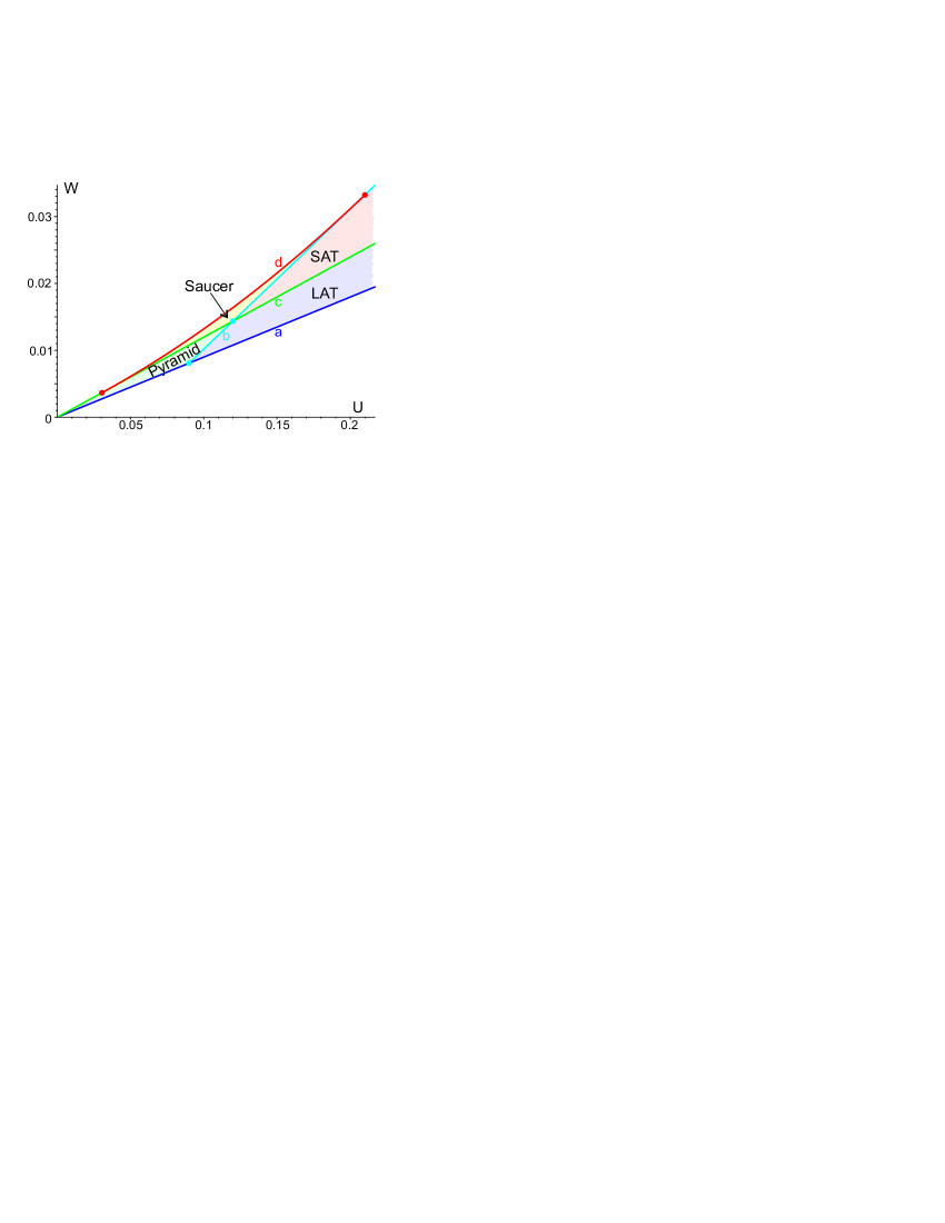
Figure 4.— Regions in the $U-W$ plane occupied by the different orbit families. Lower (dark blue) line ($a$), equation (29); upper (red) curve ($d$), equation  (34); green line ($c$), equation (30); light blue line ($b$), equation (31); red points, equation (35); blue points, equation (32). Plotted for $\epsilon_{b}=0.002,\epsilon_{c}=0.008$.

While our focus is on the pyramid orbits, the low-angular-momentum Hamiltonian (15) also supports orbits from other families. In this section, we complete the discussion of the phase space described by equation (15), by delineating the regions in the $U-W$ plane that are occupied by each of the four orbit families (Figure 4).

Pyramids and LATs both resemble distorted rectangles in the $e_{x},e_{y}$ plane. The corner points of this region correspond to $\dot{e}_{x}=\dot{e}_{y}=0$. Evaluating the two integrals at a corner (denoted by the subscript $0$) gives

$$U = \nu_{x0}^{2}\,e_{x0}^{2}+\nu_{y0}^{2}\,e_{y0}^{2}+\dot{e}_{z,0}^{2}\,,$$ (28a)

$$W = \nu_{x0}^{4}\,e_{x0}^{2}+\nu_{y0}^{4}\,e_{y0}^{2}+(U-\dot{e}_{z,0}^{2})\dot{e}_{z,0}^{2}\,.$$ (28b)

The difference between pyramids and LATs arises from the last term: corner points of pyramid orbits correspond to $\ell^{2}=0$ and hence (from (21)) to $\dot{e}_{z,0}=0$. For LATs the condition is, conversely, $\dot{e}_{z,0}^{2}>0$, and $e_{z,0}=0$ (hence $e_{y0}^{2}=1-e_{x0}^{2}$). Analyzing these expressions, we find that for pyramids and LATs the lower and upper boundaries for $W$ given $U$ are

$$W = \nu_{y0}^{2}\,U\,,$$ (29)

$$W = \nu_{x0}^{2}\,U\,,$$ (30)

and the boundary between pyramids and LATs is given by

$$W=(\nu_{x0}^{2}+\nu_{y0}^{2})\,U-\nu_{x0}^{2}\,\nu_{y0}^{2}.$$ (31)

Pyramids lie above and to the left of this line in the $U-W$ plane, while LATs are below and to the right. The intersection of this line with (29) and (30) occurs at the points

$$U = \nu_{y0}^{2},\;W=\nu_{y0}^{4}\,,$$ (32a)

$$U = \nu_{x0}^{2},\;W=\nu_{x0}^{4}\,.$$ (32b)

These points constitute the leftmost bound for LATs and the rightmost bound for pyramids respectively.

Short-axis tubes and saucers resemble distorted rectangular regions in the $e_{x},e_{z}$ plane. Again, the corner points (with subscript 0) are defined to have $\dot{e}_{x}=\dot{e}_{z}=0$ and $e_{y}=0$, with $\dot{e}_{y}^{2}>0$, and therefore

$$U = \nu_{x0}^{2}\,e_{x0}^{2}+\dot{e}_{y0}^{2}\,,$$ (33a)

$$W = \nu_{x0}^{2}\,U+(\nu_{x0}^{2}e_{x0}^{2}+\nu_{y0}^{2}-\nu_{x0}^{2})\,\dot{e}_{y0}^{2}\,.$$ (33b)

Both these families have $W\geq\epsilon_{c}U$, i.e. lie above the line (30). SAT orbits intersect the plane $e_{z}=0$, so we can set $e_{x0}=1$ in (33). (Alternatively, for SATs, both angles circulate, so we can set $\varpi=\Omega=0$, which again gives $e_{x}=1$). We then find that SATs lie below the line (31).

On the other hand, saucers never reach $e_{z}=0$ (since for them $\sin^{2}\varpi>0$), so that they lie above the line (31). To obtain the upper limit for $W$ at fixed $U$, we substitute $\dot{e}_{y0}^{2}$ from the first equation in (33) in the second, and then seek a maximum of $W$ with respect to $e_{x0}$ at fixed $U$. This gives

$$W=\nu_{x0}^{2}\,U+(U+\nu_{y0}^{2}-\nu_{x0}^{2})^{2}/4.$$ (34)

This curve intersects (30) and (31) in the points

$$U=\nu_{x0}^{2}-\nu_{y0}^{2},\;W=\nu_{x0}^{2}U\,,$$ (35a)

$$U=\nu_{x0}^{2}+\nu_{y0}^{2},\;W=\nu_{x0}^{2}U+\nu_{y0}^{4}\,,$$ (35b)

which define the left- and rightmost bounds for the saucer region.

All these criteria are summarized in Figure 4. In particular, pyramid orbits exist in the following cases:

• for $0\leq H\leq\frac{5}{2}\epsilon_{b}$ they coexist with LATs;

• for $0\leq H\leq\frac{5}{2}(\epsilon_{c}-\epsilon_{b})$ they coexist with SAT saucers;

• above these values they are the only population for $H\leq\frac{5}{2}\epsilon_{c}$, which is the maximum allowed value of $H$.

• below $H<0$ pyramids do not exist (this is easily seen from equation (15): since the term in square brackets is always non-negative, it is impossible to have $\ell^{2}=0$ when $H<0$).

Figure 5 shows Poincaré surfaces of section for $\Omega=\pi/2$ and $0<H<\frac{5}{2}\epsilon_{b}$. The three families of orbits are delineated.

Since $H$ is an integral of the motion, the maximum allowed value of $\ell^{2}$ can not exceed

$$\ell_{\mathrm{max}}^{2}(H)=\frac{5\epsilon_{c}-2H}{3+4\epsilon_{c}-\epsilon_{b}}\approx\frac{1}{3}(5\epsilon_{c}-2H).$$ (36)

The latter approximate expression is immediately seen from the simplified Hamiltonian (15), while the former comes from the exact Hamiltonian (13). However, it does not follow that an orbit with a sufficiently low instantaneous value of the angular momentum is necessarily a pyramid: both tube families can also have arbitrarily low $\ell$. The principal distinction is that any pyramid orbit can achieve arbitrarily low $\ell$ (that is, the lower bound is $\ell=0$), while tube orbits always have $0<\ell_{\mathrm{min}}^{2}\leq\ell^{2}$ (however small $\ell_{\mathrm{min}}$ may be, it is strictly positive).

We now return from the simplified Hamiltonian (15) to the full Hamiltonian (13), i.e. we no longer require $\epsilon$ to be small. The full Hamiltonian retains all the qualitative properties of the simplified system but requires numerical integration of the equations of motion (13) to determine orbit classes.

To quantify the overall fraction of pyramid orbits in a given potential, one should uniformly sample the phase space for all four variables and determine the orbit class for each initial condition. From equation (36), we can restrict ourselves to values of $\ell^{2}\leq\ell_{\mathrm{max}}^{2}(0)=\frac{5\epsilon_{c}}{3+4\epsilon_{c}-\epsilon_{b}}$ (but we must take care not to filter out initial conditions corresponding to $H<0$).

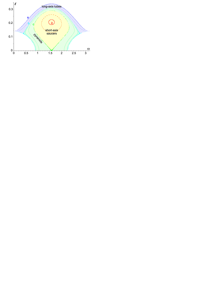
Figure 5.— Poincaré section for $\ell,\varpi$ plotted at $\Omega=\pi/2$ for energy $H=0.02$ ($\epsilon_{b}=0.99^{-2}-1,\epsilon_{c}=0.96^{-2}-1$) showing the three possible types of orbit: LATs, pyramids and SATs/saucers. This figure adopts the same potential parameters as Figure 5b in Sambhus & Sridhar (2000), but those authors chose $H=-0.02$ which precludes pyramid orbits. Boundaries are marked by the same letters as in Figure 4.

We calculated the proportions of the $\ell_{\mathrm{max}}^{2}$-restricted fraction of phase space occupied by each family of orbits. Initial conditions were drawn randomly for $10^{4}$ points (with uniform distribution in $\ell^{2}\in[0..\ell^{2}_{max}]$, in $\ell_{z}\in[0..\ell]$, and in $\varpi,\Omega\in[0,\frac{\pi}{2}]$). The proportions were found to depend very weakly on $\epsilon_{c}$ if $\epsilon_{c}\ll 1$. To elucidate the dependence on $\epsilon_{b}/\epsilon_{c}$ (the degree of triaxiality) we took 15 values in the range ($0.001-0.999$).

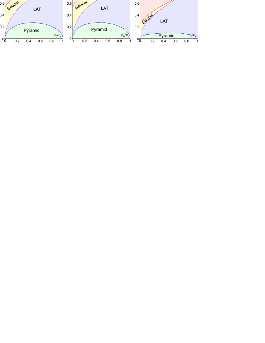
Figure 6.— Proportions of the restricted part of phase space (defined by $\ell^{2}<\ell_{\mathrm{max}}^{2}(0)$) that are occupied by the major orbit families: LATs, pyramids, SATs, and SAT/saucers, as a function of the ratio $\epsilon_{b}/\epsilon_{c}$. Left: analytic estimates from the simplified orbit-averaged Hamiltonian (15) for $\epsilon_{c}\to 0$; middle: orbit-averaged Hamiltonian (13) for $\epsilon_{c}=0.1$; right: real-space integration for orbits with semimajor axis $a=r_{\mathrm{infl}}$ (equal to the BH influence radius) and $\epsilon_{c}=0.1$.

We found that the relative fraction $\eta$ of pyramids among low-$\ell$ orbits is almost independent of $\epsilon_{c}$ (Figure 6):

$$\eta\approx 0.28\sqrt{4\frac{\epsilon_{b}}{\epsilon_{c}}\left(1-\frac{\epsilon_{b}}{\epsilon_{c}}\right)}.$$ (37)

The fraction of pyramids among all orbits is $\tilde{\eta}=\eta\ell_{\mathrm{max}}^{2}(0)=\frac{5}{3}\epsilon_{c}\,\eta$. For comparison, the left panel of Figure 6 shows the results obtained using the simplified Hamiltonian (15) and the analytical classification scheme described above, while the middle panel, made for $\epsilon_{c}=0.1$, shows almost the same behavior, with the addition of a small number of chaotic orbits. We note that for $\epsilon_{c}\sim 1$ the phase space becomes largely chaotic.

These estimates of the relative fraction of pyramid orbits are directly applicable to a galaxy with an isotropic distribution of stars at any energy. This assumption may not be valid, for example, in the case of induced tangential anisotropy following the merger of supermassive BHs (Merritt & Milosavljevic, 2005).

One can ask a different question: if we know the instantaneous value of an orbit’s eccentricity and orientation, what can we conclude about the orbit class? It is clear that without knowledge of the derivatives of $e_{x,y}$ the answer will only be probabilistic. It turns out that the probability $p$ for an orbit with “sufficiently high” eccentricity (i.e. with $\ell^{2}\leq\ell_{\mathrm{max}}^{2}$) to be a pyramid depends mostly on the $z$ component of the eccentricity vector: $p\approx 0.7\sqrt{4\frac{\epsilon_{b}}{\epsilon_{c}}(1-\frac{\epsilon_{b}}{\epsilon_{c}})}\,e_{z}^{1.5}$ (here the normalization comes from the total number of pyramids among low-$\ell$ orbits). That is, an orbit lying in the plane defined by the long and intermediate axes of the potential is certainly not a pyramid, and the highest probabilitiy occurs for orbits directed toward the short axis.

4.4. Large $\ell$ limit

In the previous sections we considered the case $\epsilon_{b,c}\ll 1$ and $\ell^{2}\sim\epsilon_{c}$, which allowed a simplification leading to integrable equations.

In the opposite case, when $\epsilon_{b,c}\ll\ell^{2}\lesssim 1$, the frequency of in-plane precession, $\nu_{\varpi}$, is much greater than the rates change of $\Omega$ and $i$ (Figure 2). In this limit we can carry out a second averaging of the Hamiltonian (13a), this time over $\varpi$. Thus

$$\langle H\rangle = \frac{1}{2\pi}\int_{0}^{2\pi}Hd\varpi=-\frac{3}{2}\ell^{2}$$

$$+ \frac{5-3\ell^{2}}{4}\left[\epsilon_{b}\left(s_{\Omega}^{2}+c_{i}^{2}c_{\Omega}^{2}\right)+\epsilon_{c}\left(5-3\ell^{2}\right)\left(1-c_{i}^{2}\right)\right].$$

On timescales $T\gtrsim\nu_{p}^{-1}$ the orbit resembles an annulus that lies in the plane defined by the angles $i$ and $\Omega$. The only remaining equations of motion are those that describe the change in orientation of the orbital plane:

$$\frac{d\ell_{z}}{d\tau} = -\frac{\epsilon_{b}}{4}\left(5-3\ell^{2}\right)\left(1-c_{i}^{2}\right)s_{2\Omega},$$ (39)

$$\ell\frac{d\Omega}{d\tau} = \frac{\epsilon_{b}}{2}\left(5-3\ell^{2}\right)c_{\Omega}^{2}c_{i}-\frac{\epsilon_{c}}{2}\left(5-3\ell^{2}\right)c_{i}.$$

One expects the natural variables in this case to be the components of the angular momentum:

$$\ell_{x} = \ell\sin i\sin\Omega,$$ (40)

$$\ell_{y} = \ell\sin i\cos\Omega,$$

$$\ell_{z} = \ell\cos i$$

and $\ell_{x}^{2}+\ell_{y}^{2}+\ell_{z}^{2}=\ell^{2}=$ constant. In terms of these variables, the Hamiltonian is

$$\langle H\rangle=-\frac{3}{2}\ell^{2}+\frac{(5-3\ell^{2})}{4\ell^{2}}\left[\epsilon_{b}\left(\ell^{2}-\ell_{y}^{2}\right)+\epsilon_{c}\left(\ell^{2}-\ell_{z}^{2}\right)\right].$$ (41)

After some algebra, one finds the equations of motion:

$$\dot{\ell}_{x} = -\frac{1}{2}\left(\epsilon_{c}-\epsilon_{b}\right)\left(5-3\ell^{2}\right)\frac{\ell_{y}\ell_{z}}{\ell^{2}},$$ (42)

$$\dot{\ell}_{y} = \frac{\epsilon_{c}}{2}\left(5-3\ell^{2}\right)\frac{\ell_{x}\ell_{z}}{\ell^{2}},$$

$$\dot{\ell}_{z} = -\frac{\epsilon_{b}}{2}\left(5-3\ell^{2}\right)\frac{\ell_{x}\ell_{y}}{\ell^{2}}$$

(only two of which are independent). These can be written

$$\frac{\mathrm{d}\vec{\ell}}{\mathrm{d}\tau} = \mathbf{T}\times\vec{\ell},$$ (43)

$$\mathbf{T} = \frac{5-3\ell^{2}}{2\ell^{2}}\left(\begin{array}[]{c}0\\ \epsilon_{b}\ell_{y}\\ \epsilon_{c}\ell_{z}\end{array}\right).$$ (47)

Conservation of the Hamiltonian (41) implies

$$\epsilon_{b}\ell_{y}^{2}+\epsilon_{c}\ell_{z}^{2}=\mathrm{constant}=C.$$

This is an elliptic cylinder; the axis is parallel to the $\ell_{x}$-axis, and the ellipse is elongated in the direction of the $\ell_{y}$-axis. In addition, we know that

$$\ell_{x}^{2}+\ell_{y}^{2}+\ell_{z}^{2}=\mathrm{constant}=\ell^{2}$$

which is a sphere. So, the motion lies on the intersection of a sphere with an elliptic cylinder. There are two possibilities.

1. $\ell^{2}>C/\epsilon_{b}$. In this case, the cylinder intersects the sphere in a deformed ring that circles the $\ell_{x}$-axis. This corresponds to a LAT orbit.

2. $\ell^{2}<C/\epsilon_{b}$. In this case, the locus of intersection is a deformed ring about the $\ell_{z}$-axis. This orbit is a SAT.

In other words, precession of the angular momentum vector can be either about the short or long (not intermediate) axes of the triaxial ellipsoid.

5. Capture of pyramid orbits by the BH

As we have seen, pyramid orbits can attain arbitrarily low values of the dimensionless angular momentum $\ell$. The BH tidally disrupts or captures stars with angular momentum less than a certain critical value $L_{\bullet}$, or – in dimensionless variables – $\ell_{\bullet}\equiv L_{\bullet}/I(a)$. We can express $\ell_{\bullet}$ in terms of the capture radius $r_{t}$, the radius at which a star is either tidally disrupted or swallowed. For BH masses greater than $\sim 10^{8}~{}M_{\odot}$, main sequence stars avoid disruption and $r_{t}\approx r_{\mathrm{Schw}}\equiv 2GM_{\bullet}/c^{2}$; for smaller $M_{\bullet}$, tidal disruption occurs outside the Schwarzschild radius; e.g. at the center of the Milky Way, $r_{t}\approx 10r_{\mathrm{Schw}}$ for solar-type stars. Defining $r_{t}=\Theta r_{\mathrm{Schw}}$ and writing $L_{\bullet}^{2}\approx G{M_{\bullet}}r_{t}$, then gives

$$\ell_{\bullet}^{2}=\Theta\,\frac{r_{\mathrm{Schw}}}{a}\approx 10^{-5}\Theta\left(\frac{M_{\bullet}}{10^{8}M_{\odot}}\right)\left(\frac{a}{1\ \mathrm{pc}}\right)^{-1}.$$ (48)

We note the following property of the pyramid orbits: as long as the frequencies of $e_{x}$ and $e_{y}$ oscillation are incommensurate, the vector $(e_{x},e_{y})$ fills densely the whole available area, which has the form of distorted rectangle. The corner points correspond to zero angular momentum, and the “drainage area” is similar to four holes in the corners of a billiard table.

Unless otherwise noted, in this section we adopt the simple harmonic oscillator (SHO) approximation to the ($e_{x},e_{y}$) motion, that is, we use the simplified Hamiltonian (15) and its solutions (23); these orbits have $e_{x}^{2}+e_{y}^{2}\ll 1$ and they form a rectangle in the $e_{x}-e_{y}$ plane, with sides $2e_{x},2e_{y}$. As long as the motion is integrable, the results for arbitrary pyramids with $e_{x},e_{y}\lesssim 1$ will be qualitatively similar. Quantitative results may be obtained by numerical analysis and are presented near the end of this section.

Figure 7 shows a two-torus describing oscillations in ($e_{x},e_{y}$) for a pyramid orbit. In the SHO approximation, solutions are given by (23). If the two frequencies $\nu_{x0},\nu_{y0}$ are incommensurate, the motion will fill the torus. In this case, we are free to shift the time coordinate so as to make both phase angles $(\phi_{1},\phi_{2})$ zero, yielding

$$\ell^{2}(\tau) = \ell_{x0}^{2}\sin^{2}(\nu_{x0}\tau)+\ell_{y0}^{2}\sin^{2}(\nu_{y0}\tau)$$ (49a)

$$= \ell_{x0}^{2}\sin^{2}\theta_{1}+\ell_{y0}^{2}\sin^{2}\theta_{2}$$ (49b)

where $\theta_{1}=\nu_{x0}\tau,\theta_{2}=\nu_{y0}\tau$. (In the case of exact commensurability, i.e. $m_{1}\nu_{x0}+m_{2}\nu_{y0}=0$ with ($m_{1},m_{2}$) integers, the trajectory will avoid certain regions of the torus and such a shift may not be possible.) In the SHO approximation, $\nu_{x0}=\sqrt{15\epsilon_{c}},\nu_{y0}=\sqrt{15(\epsilon_{c}-\epsilon_{b})}$ (22). More generally, integrable motion will still be representable as uniform motion on the torus but the frequencies and the relations between $\ell$ and the angles will be different.

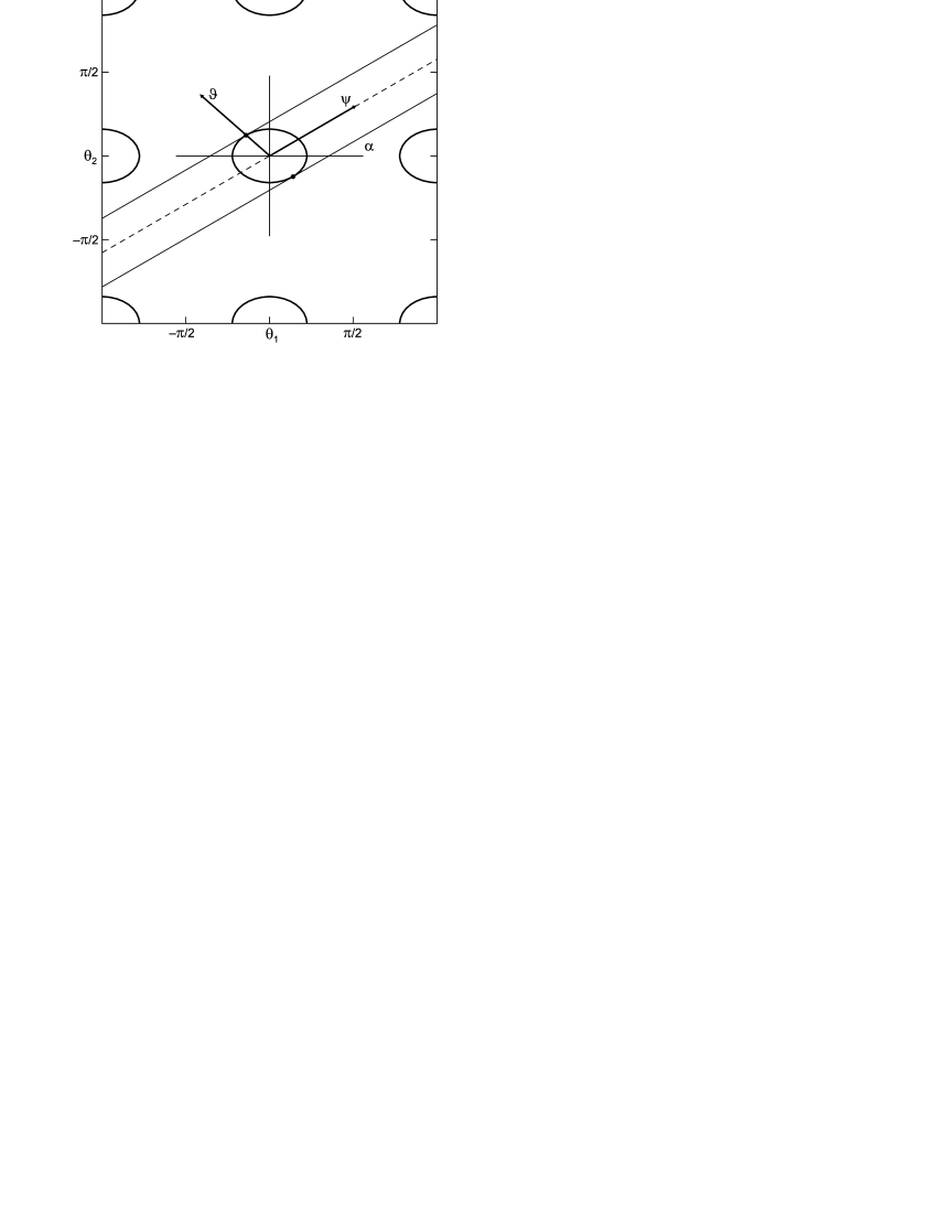
Figure 7.— Two-torus describing oscillations of ($e_{x},e_{y}$) for a pyramid orbit. The ellipses correspond to regions near the four corners of the pyramid’s base where $\ell\leq\ell_{\bullet}$. In the orbit-averaged approximation, trajectories proceed smoothly along lines parallel to the solid lines, with slope $\tan\alpha=\nu_{y}/\nu_{x}$. In reality, successive periapse passages occur at discrete intervals, once per radial period.

Stars are lost when $\ell(\theta_{1},\theta_{2})\leq\ell_{\bullet}$. Consider the loss region centered at $(\theta_{1},\theta_{2})=(0,0)$. This is one of four such regions, of equal size and shape, that correspond to the four corners of the base of the pyramid. For small $\ell_{\bullet}$, the loss region is approximately an ellipse,

$$\frac{\ell_{x0}^{2}}{\ell_{\bullet}^{2}}\theta_{1}^{2}+\frac{\ell_{y0}^{2}}{\ell_{\bullet}^{2}}\theta_{2}^{2}\lesssim 1.$$ (50)

The area enclosed by this “loss ellipse” is

$$\pi\frac{\ell_{\bullet}^{2}}{\ell_{x0}\ell_{y0}}.$$ (51)

There are four such regions on the torus; together, they constitute a fraction

$$\mu=\frac{1}{\pi}\frac{\ell_{\bullet}^{2}}{\ell_{x0}\ell_{y0}}$$ (52)

of the torus.

Stars move in the $(\theta_{1},\theta_{2})$ plane along lines with slope $\tan\alpha=\nu_{y0}/\nu_{x0}$, at an angular rate of $\sqrt{\nu_{x0}^{2}+\nu_{y0}^{2}}$. Since periapse passages occur only once per radial period, a star will move a finite step in the phase plane between encounters with the BH. The dimensionless time between successive periapse passages is $\Delta t=2\pi\nu_{p}/\nu_{r}$. The angle traversed during this time is

$$\Delta\theta=2\pi(\nu_{p}/\nu_{r})\sqrt{\nu_{x0}^{2}+\nu_{y0}^{2}}.$$ (53)

The rate at which stars move into one the four loss ellipses is given roughly by the number of stars that lie an angular distance $\Delta\theta$ from one side of a loss ellipse, divided by $\Delta t$.

This is not quite correct however, since a star may precess past the loss ellipse before it has had time to reach periapse. We carry out a more exact calculation by assuming that the torus is uniformly populated at some initial time, with unit total number of stars. To simplify the calculation, we transform to a new phase plane defined by

$$\psi = \frac{\nu_{x0}\ell_{x0}^{2}\theta_{1}+\nu_{y0}\ell_{y0}^{2}\theta_{2}}{\sqrt{\nu_{x0}^{2}\ell_{x0}^{2}+\nu_{y0}^{2}\ell_{y0}^{2}}},$$ (54)

$$\vartheta = \frac{-\nu_{y0}\ell_{x0}\ell_{y0}\theta_{1}+\nu_{x0}\ell_{x0}\ell_{y0}\theta_{2}}{\sqrt{\nu_{x0}^{2}\ell_{x0}^{2}+\nu_{y0}^{2}\ell_{y0}^{2}}}.$$ (55)

With this transformation, the phase velocity becomes

$$\dot{\psi}=(\nu_{x0}^{2}\ell_{x0}^{2}+\nu_{y0}^{2}\ell_{y0}^{2})^{1/2},\ \ \ \ \ \ \dot{\vartheta}=0$$ (56)

and the loss regions become circles of radius $\ell_{\bullet}$. The angular displacement in one radial period is

$$\Delta\psi=2\pi(\nu_{p}/\nu_{r})\left(\nu_{x0}^{2}\ell_{x0}^{2}+\nu_{y0}^{2}\ell_{y0}^{2}\right)^{1/2}.$$ (57)

The density of stars is $(4\pi^{2}\ell_{x0}\ell_{y0})^{-1}$.

At any point in the ($\psi,\vartheta$) plane, stars have a range of radial phases. Assuming that the initial distribution satisfies Jeans’ theorem, stars far from the loss regions are uniformly distributed in $\chi$ where

$$\chi=P^{-1}\int_{r_{p}}^{r}\frac{dr}{v_{r}};$$ (58)

here $P\equiv 2\pi/\nu_{r}$ is the radial period, $r_{p}$ is the periapse distance and $v_{r}$ is the radial velocity. The integral is performed along the orbit, hence $\chi$ ranges between 0 and 1 as $r$ varies from $r_{p}$ to apoapse and back to $r_{p}$. ($\chi=w\mbox{ mod }2\pi$, where $w$ is mean anomaly).

Figure 8 shows how stars move in the $(\chi,\psi)$ plane at fixed $\vartheta$. The loss region extends in $\psi$ a distance $2\sqrt{\ell_{\bullet}^{2}-\vartheta^{2}}$, from $\psi_{\mathrm{in}}$ to $\psi_{\mathrm{out}}$. Stars are lost to the BH if they reach periapse while in this region.

Two regimes must be considered, depending on whether $\Delta\psi$ is less than or greater than $\psi_{\mathrm{out}}-\psi_{\mathrm{in}}$.

1. $\Delta\psi<\psi_{\mathrm{out}}-\psi_{\mathrm{in}}$ (Figure 8a). In one radial period, stars in the orange region are lost. One-half of this region lies within the loss ellipse; these are stars with $\ell<\ell_{0}$ but which have not yet attained periapse. The persistence of stars inside the “loss cone” is similar to what occurs in the case of diffusional loss cone repopulation, where there is also a “boundary layer”, the width of which depends on the ratio of the relaxation time to the radial period (e.g. Cohn & Kulsrud (1978)). The other one-half consists of stars that have not yet entered the loss region. The area of the orange region is equal to the area of a rectangle of unit height and width $\Delta\psi$; since stars are distributed uniformly on the $(\chi,\psi)$ plane, the number of stars lost per radial period is equal to the total number of stars, of any radial phase, contained within $\Delta\psi$.

2. $\Delta\psi>\psi_{\mathrm{out}}-\psi_{\mathrm{in}}$ (Figure 8b). In this case, some stars manage to cross the loss region without being captured. The area of the orange region is equal to that of a rectangle of unit height and width $\psi_{\mathrm{out}}-\psi_{\mathrm{in}}$. The number of stars lost per radial period is therefore equal to the number of stars, of arbitrary radial phase, contained within $\psi_{\mathrm{out}}-\psi_{\mathrm{in}}=2\sqrt{\ell_{\bullet}^{2}-\vartheta^{2}}$.

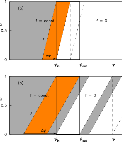
Figure 8.— Trajectories of stars in the $(\psi,\chi)$ plane as they encounter a loss region from left to right, defined as $\psi_{\mathrm{in}}\leq\psi\leq\psi_{\mathrm{out}}$. $\chi$ increases from 0 at periapse, to $1/2$ at apoapse, to $1$ at subsequent periapse. Trajectories are indicated by dashed lines. Stars are lost if they reach periapse while inside the loss region. Stars within the orange region are lost in one radial period. (a) $\Delta\psi<\psi_{\mathrm{in}}-\psi_{\mathrm{out}}$; (b) $\Delta\psi>\psi_{\mathrm{in}}-\psi_{\mathrm{out}}$.

To compute the total loss rate, we integrate the loss per radial period over $\vartheta$. It is convenient to express the results in terms of $q$ where

$$q\equiv\frac{\Delta\psi}{2\ell_{\bullet}}=\pi\frac{\nu_{p}}{\nu_{r}}\ell_{\bullet}^{-1}\sqrt{\nu_{x0}^{2}\ell_{x0}^{2}+\nu_{y0}^{2}\ell_{y0}^{2}}.$$ (59)

$q\ll 1$ corresponds to an “empty loss cone” and $q\gg 1$ to a “full loss cone”. However we note that – for any $q<1$ – there are values of $\vartheta$ such that the width of the loss region, $\psi_{\mathrm{out}}-\psi_{\mathrm{in}}$, is less than $\Delta\psi$. In terms of the integral $W$ defined above (28), $q$ becomes simply

$$q=\frac{P\nu_{p}}{6\ell_{\bullet}}\sqrt{W}.$$ (60)

Unlike the case of collisional loss cone refilling, where $q=q(E)$ is only a function of energy, here $q$ is also a function of a second integral $W$. Pyramid orbits with small opening angles will have small $W$ and small $q$.

The area on the $(\psi,\vartheta)$ plane that is lost, in one radial period, into one of the four loss regions is

$$2\int_{0}^{\vartheta_{c}}\Delta\psi d\vartheta+2\int_{\vartheta_{c}}^{\ell_{\bullet}}(\psi_{\mathrm{out}}-\psi_{\mathrm{in}})d\vartheta$$ (61)

where

$$\vartheta_{c}\equiv\ell_{\bullet}\sqrt{1-q^{2}}$$ (62)

is the value of $\vartheta$ where $\Delta\psi=\psi_{\mathrm{out}}-\psi_{\mathrm{in}}$; for $q\geq 1$, $\vartheta_{c}=0$. For $q\leq 1$, the area integral becomes

$$4q\ell_{\bullet}\int_{0}^{\vartheta_{c}}d\vartheta+4\int_{\vartheta_{c}}^{\ell_{\bullet}}\sqrt{\ell_{\bullet}^{2}-\vartheta^{2}}d\vartheta$$

$$= 4q\ell_{\bullet}^{2}\sqrt{1-q^{2}}\ +4\ell_{\bullet}^{2}\int_{\sqrt{1-q^{2}}}^{1}dx\sqrt{1-x^{2}}$$

$$= \ell_{\bullet}^{2}\left(\pi+2q\sqrt{1-q^{2}}-2\arcsin\sqrt{1-q^{2}}\right)$$

$$= 4q\ell_{\bullet}^{2}f(q),$$

$$f(q) = \frac{1}{2}\sqrt{1-q^{2}}+\frac{1}{2q}\arcsin(q)$$ (63)

and for $q>1$ it is $\pi\ell_{\bullet}^{2}$. The function $f(q)$ varies from $f(0)=1$ to $f(1)=\pi/4\approx 0.785$.

The area on the phase plane that is lost each radial period can be interpreted in a very simple way geometrically, as shown in Figure 9.

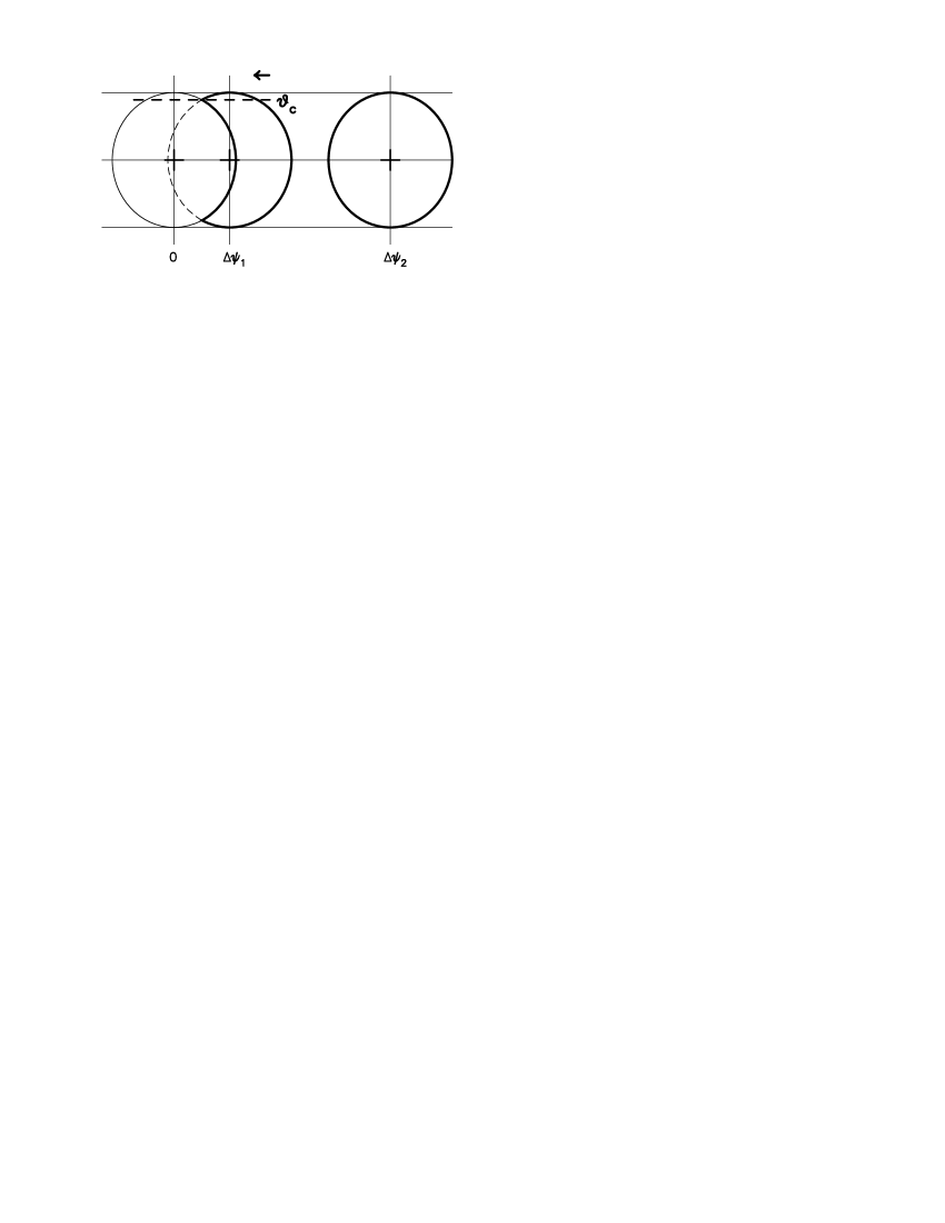
Figure 9.— Illustrating the area of the $(\psi,\vartheta)$ phase plane that is lost into the BH each radial period. The circle centered at $(0,0)$ is the loss region corresponding to one corner of the pyramid orbit; its radius is $\ell_{\bullet}$. Regions marked in bold denote the area of the torus that is lost in one radial period, for $q<1$ ($\Delta\psi_{1}$) and $q>1$ ($\Delta\psi_{2}$). While the number of stars lost per radial period is proportional to the marked areas, the region on the torus from which those stars come is more complicated since it depends also on an orbit’s radial phase (Figure 8).

Considering that there are four loss regions, the instantaneous total loss rate $\cal F$, in dimensionless units, is

$${\cal F} = f(q)\frac{2\ell_{\bullet}}{\pi^{2}\,\ell_{x0}\ell_{y0}}\sqrt{\nu_{x0}^{2}\,\ell_{x0}^{2}+\nu_{y0}^{2}\,\ell_{y0}^{2}}=\frac{\mu}{P\nu_{p}}\frac{4q\,f(q)}{\pi}$$ (64a)

$$\mbox{for }0\leq q\leq 1,$$

$${\cal F} = q^{-1}\frac{\ell_{\bullet}}{2\pi\,\ell_{x0}\ell_{y0}}\sqrt{\nu_{x0}^{2}\,\ell_{x0}^{2}+\nu_{y0}^{2}\,\ell_{y0}^{2}}=\frac{1}{2\pi^{2}}\frac{\ell_{\bullet}^{2}}{\ell_{x0}\ell_{y0}}\frac{\nu_{r}}{\nu_{p}}$$ (64b)

$$= \frac{\mu}{P\nu_{p}}\ \ \ \ \mbox{for }q>1.$$

The second expression for the loss rate, equation (64b), can be called the “full-loss-cone” loss rate, since it corresponds to completely filling and empyting the loss regions in each radial step (Figure 9). Note that the loss rate for $q<1$ is $\sim q$ times the full-loss-cone loss rate. A similar relation holds in the case of collisionally repopulated loss cones (Cohn & Kulsrud, 1978).

The inverse of the loss rate $\cal F$ gives an estimate of the time $t_{\mathrm{drain}}$ required to drain an orbit, or equivalently the time for a single star, of unknown initial phase, to go into the BH. In this approximation, the loss rate remains constant until $t=t_{\mathrm{drain}}$ at which time the torus is completely empty. In reality the draining time will always be longer than this, since after $\sim 1$ precessional periods, some parts of the torus that are entering the loss regions will be empty and the loss rate will drop below equation (64). For $\Delta\psi\geq\psi_{\mathrm{in}}-\psi_{\mathrm{out}}$, the downstream density in Figure 8, integrated over radial phase, is easily shown to be $1-q^{-1}\sqrt{1-\vartheta^{2}/\ell_{\bullet}^{2}}$ times the upstream density while for $\Delta\psi<\psi_{\mathrm{in}}-\psi_{\mathrm{out}}$ the downstream density is zero. Integrated over $\vartheta$, the downstream depletion factor becomes

$$1-\frac{\pi}{4q}-\sqrt{1-q^{2}}(1+q)+\frac{1}{2q}\sin^{-1}\sqrt{1-q^{2}}$$ (65)

for $q\leq 1$ and $1-\pi/4q$ for $q>1$; it is $0$ for $q=0$, $\sim 0.215$ for $q=1$ and $1$ for $q\rightarrow\infty$. For small $q$, the torus will become striated, containing strips of nearly-zero density interlaced with undepleted regions; the loss rate will exhibit discontinous jumps whenever a depleted region encounters a new loss ellipse and the time to totally empty the torus will depend in a complicated way on the frequency ratio $\nu_{x}/\nu_{y}$ and on $\ell_{\bullet}$. For large $q$, the loss rate will drop more smoothly with time, roughly as an exponential law with time constant $\sim t_{\mathrm{drain}}$.

We postpone a more complete discussion of loss cones in the triaxial geometry to a future paper. Here we make a few remarks about pyramids with arbitrary opening angles, i.e. for which $e_{x0},e_{y0}$ are not required to be small.

For each orbit one can compute $\mu$, the fraction of the torus occupied by the loss cone (equation 52), by numerically integrating the equations of motion (13) and analyzing the probability distribution for instantaneous values of $\ell^{2}$: ${\cal P}(\ell^{2}<X)\propto X-\ell_{min}^{2}$, where $\ell_{min}^{2}$ allows for a nonzero lower bound on $\ell^{2}$. Almost all pyramids have $\ell_{min}=0$, but some of them happen to be resonances (commensurable $\nu_{x}$ and $\nu_{y}$) and hence avoid approaching $\ell=0$. This linear character of the distribution of $\ell^{2}$ near its minimum corresponds to a linear probability distribution of periapse radii (${\cal P}(r_{\mathrm{peri}}<r)\propto r$), which is natural to expect if we combine a quadratic distribution of impact parameters at infinity with gravitational focusing (see equation 7 of Merritt & Poon (2004)).

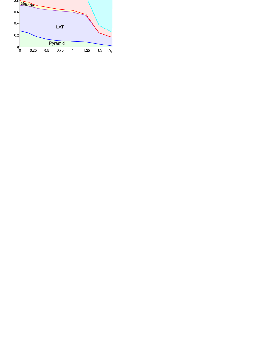
Figure 10.— Proportion of phase space ($\ell^{2}<\ell_{\mathrm{max}}^{2}(0)$) that is occupied by the major orbit families: LATs, pyramids, SATs, saucers, and chaotic orbits, as a function of semimajor axis $a$ based on real-space integrations. Triaxiality parameters are $\epsilon_{b}=0.5\epsilon_{c}$ and $\epsilon_{c}=0.12/[0.2+(a/r_{\mathrm{infl}})^{-1}]$ (equation 11), corresponding to a density cusp with $\gamma=1$ and $\epsilon_{c}=0.1$ at $a=r_{\mathrm{infl}}$. For $a\gtrsim r_{\mathrm{infl}}$ most low-$\ell$ orbits are chaotic (Poon & Merritt, 2001).

The coefficient $\mu$ for each orbit is calculated as ${\cal P}(\ell^{2}<\ell_{\bullet}^{2})$. As seen from equation (52), the smaller the extent of a pyramid in any direction, the greater $\mu$ – this is true even for orbits with large $e_{x0}$ or $e_{y0}$. While $\mu$ varies greatly from orbit to orbit, its overall distribution over the entire ensemble of pyramid orbits follows a power law:

$${\cal P}_{\mu}(\mu>Y)\approx(Y/\mu_{min})^{-2}\;,\qquad\mu_{min}\approx\frac{\ell_{\bullet}^{2}}{2\tilde{\eta}};$$ (66)

${\cal P}_{\mu}$ is the probability of having $\mu$ greater than a certain value and $\tilde{\eta}$ is the fraction of pyramids among all orbits (37). The average $\mu$ for all pyramid orbits is therefore $\overline{\mu}=2\mu_{min}$, and the average fraction of time that a random orbit of any type and any $\ell$ spends inside the loss cone is $\overline{\mu}\tilde{\eta}\simeq\ell_{\bullet}^{2}$ (almost independent of the potential parameters $\epsilon_{b}$ and $\epsilon_{c}$) – the same number that would result from an isotropic distribution of orbits in a spherically-symmetric potential.

6. Comparison with real-space integrations

We tested the applicability of the orbit-averaged approach by comparing the orbit-averaged equations of motion, equation (13b), with real-space integrations of orbits having the same initial conditions (and arbitrary radial phases). The agreement was found to be fairly good for orbits with semimajor axes $a\lesssim 0.1r_{\mathrm{infl}}$: about 90% of the orbits were found to belong to the same orbital class, and the correspondence between values of $\mu$ and $\ell_{\mathrm{min}}^{2}$ was also quite good for individual orbits. Averaged over the ensemble, the proportion of phase space occupied by the different orbital families, as well as the net flux of pyramids into the BH, is almost the same for the two methods. However, at larger radii, the relative fraction of pyramids and saucers decreases (Figure 6 (right), 10). Since the maximum possible angular momentum for orbits with a given semimajor axis $a$ grows faster than $\sqrt{G{M_{\bullet}}a}$, this means that the fraction of pyramid orbits among all (not just low-$\ell$) orbits is even smaller. For orbits with semimajor axis $a\gtrsim r_{\mathrm{infl}}$ the frequency of radial oscillation becomes comparable to the frequencies of precession, and when these overlap, orbits tend to become chaotic. (Weakly chaotic behavior starts earlier). So low-$\ell$ orbits with $a>1.5r_{\mathrm{infl}}$ are mostly chaotic, as seen from Figure 10, confirming that regular pyramid orbits (along with saucers) exist only within BH sphere of influence (Poon & Merritt, 2001).

7. Effects of general relativity

In the previous sections we considered the BH as a Newtonian point mass. In general relativity (GR), the gravitational field of the BH is more complicated, and this will affect the behavior of orbits with distances of closest approach that are comparable to $r_{g}\equiv GM_{\bullet}/c^{2}$.

For a non-spinning BH, the lowest order post-Newtonian effect is advance of the periapse, which acts in the opposite sense to the precession due to an extended mass distribution. The GR periapse advance is

$$\Delta\varpi=\frac{6\pi}{c^{2}}\frac{G{M_{\bullet}}}{(1-e^{2})a}$$ (67)

per radial period, with $c$ the speed of light (Weinberg, 1972), making the orbit-averaged precession frequency

$$\nu_{GR}=\nu_{r}\frac{3GM_{\bullet}}{c^{2}\,a\,\ell^{2}}.$$ (68)

We can approximate the effects of this precession by adding an extra term to the orbit-averaged Hamiltonian (13):

$$H = -\frac{3}{2}\ell^{2}+\epsilon_{b}H_{b}+\epsilon_{c}H_{c}-\frac{\varkappa}{\ell}$$ (69a)

$$\varkappa \equiv \frac{\nu_{GR}\ell^{2}}{\nu_{p}}=\frac{3G{M_{\bullet}}}{c^{2}a}\frac{\nu_{r}}{\nu_{p}}\sim\frac{r_{\mathrm{Schw}}}{a}\frac{M_{\bullet}}{M(a)}.$$ (69b)

This is equivalent to adding the term $\varkappa/l^{2}$ to the equation of motion for $\varpi$, i.e. to the right hand side of $d\varpi/d\tau=\partial H/\partial\ell$. When $\ell=\ell_{\mathrm{crit}}$, where

$$\ell_{\mathrm{crit}}=\left(\frac{\varkappa}{3}\right)^{1/3},$$ (70)

the precession due to GR exactly cancels the precession due to the spherical component of the distributed mass. Since the angular momentum of a pyramid orbit approaches arbitrarily close to zero in the absence of GR, there will always come a time when its precession is dominated by the effects of GR, no matter how small the value of the dimensionless coefficient $\varkappa$.

We again restrict consideration to the simplified Hamiltonian (15), valid for $\epsilon_{b},c\ll 1$, $\ell^{2}\lesssim\epsilon_{c}$, now with the added term due to GR. This Hamiltonian may be rewritten as

$$\frac{5}{2}\epsilon_{c}-H = \left[\frac{3}{2}\ell^{2}+\frac{\varkappa}{\ell}\right]+\left[\frac{5}{2}\epsilon_{c}e_{x}^{2}+\frac{5}{2}(\epsilon_{c}-\epsilon_{b})e_{y}^{2}\right]$$ (71)

$$\equiv P(\ell)+Q(e_{x},e_{y})\,,$$

where $P$ and $Q$ denote the expressions in the first and second sets of square brackets. The minimum of $P(\ell)$ occurs at $\ell=\ell_{\mathrm{crit}}$:

$$P_{\mathrm{min}}=\sqrt[3]{81\varkappa^{2}/8}.$$ (72)

The function $Q$ can vary from 0 to some maximum value $Q_{\mathrm{max}}$ due to the limitation that $e_{x}^{2}+e_{y}^{2}\leq 1$.

Two differences from the Newtonian case are apparent.

1) For each value of $(e_{x},e_{y})$ (and therefore $Q$), there are now two allowed values of $\ell$. One of these is smaller than $\ell_{\mathrm{crit}}$ while the other is greater (Figure 11).

2) Both the minimum and maximum values of $\ell$ – both of which correspond to the maximum value of $P$ (Figure 11) – are attained when $Q=0$, i.e. when $e_{x}=e_{y}=0$. The maximum of $Q$ corresponds to $\ell=\ell_{\mathrm{crit}}$. In the Newtonian case, the minimum of $\ell$ corresponds to the maximum of $Q$.

7.1. Planar orbits

We first consider orbits confined to the $y-z$ plane ($e_{x}=0$, hence $\Omega=\pi/2,\ell_{z}=0$ throughout the evolution). Namely, we start an orbit from $\varpi=\pi/2$ ($e_{y}=0$) and $\ell=\ell_{0}$. In the absence of GR, such an orbit would be a LAT for $\ell_{0}>\frac{5}{3}\epsilon_{b}$ and a pyramid otherwise.

The Hamiltonian and the equations of motion are

$$\frac{5}{2}\epsilon_{c}-H = \frac{3}{2}\ell_{0}^{2}+\frac{\varkappa}{\ell_{0}}=\frac{3}{2}\ell^{2}+\frac{\varkappa}{\ell}+\frac{\nu_{y0}^{2}}{6}\cos^{2}\varpi\,,$$ (73)

$$\dot{\ell} = -\frac{\nu_{y0}^{2}}{6}\sin 2\varpi\,,\qquad\dot{\varpi}=-3\ell+\frac{\varkappa}{\ell^{2}}\,.$$ (74)

The orbit in the course of its evolution may or may not attain $\varpi=0\ (\mathrm{mod}\,\pi)$. If it does, then the angle $\varpi$ circulates monotonically, with $\dot{\varpi}\neq 0$. In Figure 11, the condition $\dot{\varpi}=0$ corresponds to reaching the lowest point in the $P(\ell)$ curve, $\ell=\ell_{\mathrm{crit}}$. Whether this happens depends on the value of $\ell_{0}$: since the orbit starts from $Q=0$ and $P=P(\ell_{0})$, it can “descend” the $P(\ell)$ curve at most by $Q_{\mathrm{max}}=\nu_{y0}^{2}/6$. If this condition is consistent with reaching $P(\ell_{\mathrm{crit}})$, the orbit will flip to the other branch of the $P(\ell)$ curve. The condition for this to happen is

$$\frac{3}{2}\ell_{0\pm}^{2}+\frac{\varkappa}{\ell_{0\pm}}=\frac{3}{2}\ell_{\mathrm{crit}}^{2}+\frac{\varkappa}{\ell_{\mathrm{crit}}}+\frac{\nu_{y0}^{2}}{6};$$ (75)

$\ell_{0+}$ and $\ell_{0-}$ are the upper and lower positive roots of this equation.

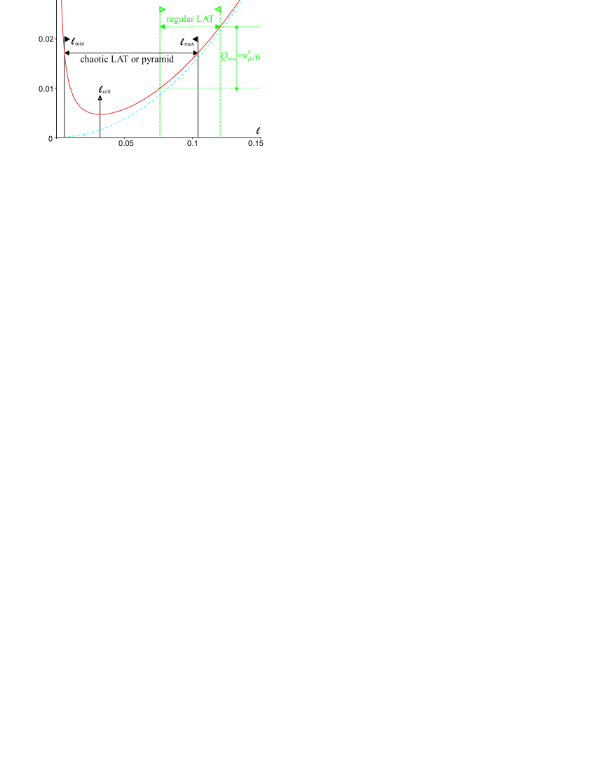
Figure 11.— Illustrating the allowed variations in angular momentum $\ell$ for orbits in the presence of general relativistic precession. The solid (red) curve represents the function $P(\ell)$ (equation 71); the dashed (blue) parabola is the same function in the Newtonian case ($\varkappa=0$). If $\varkappa\neq 0$, $P(\ell)$ has a minimum at $\ell_{\mathrm{crit}}$ (equation 70). Orbits make excursions along the curve $P(\ell)$ in the range from a certain value $P_{\mathrm{max}}$ to $P_{\mathrm{max}}-Q_{\mathrm{max}}$ (here $Q_{\mathrm{max}}$ is given for the case of planar orbits of § 7.1 and equals $\frac{5}{2}(\epsilon_{c}-\epsilon_{b})\equiv\nu_{y0}^{2}/6$). If during such an excursion $\ell$ does not cross $\ell_{\mathrm{crit}}$, then the orbit resides on one branch of $P(\ell)$, typically remaining regular. Otherwise it flips to the other branch, reaching lower values of $\ell_{\mathrm{min}}$ (equation 83), becoming a (typically chaotic) LAT or pyramid orbit.

If $\ell_{0}>\ell_{0+}$, the orbit behaves like a Newtonian LAT (Figure 12, case $a$): it has $\dot{\varpi}<0$ and $\ell>\ell_{\mathrm{crit}}$. If $\ell_{0}<\ell_{0-}$, the orbit is again a LAT, but now it precesses in the opposite direction ($\dot{\varpi}>0$) due to the dominance of GR, and $\ell$ never climbs above $\ell_{\mathrm{crit}}$ (Figure 12, case $e$). In these cases the condition $\varpi=0$ gives the extremum of $\ell$, which is found from equation (73):

$$\frac{3}{2}\ell_{\mathrm{extr,L}}^{2}+\frac{\varkappa}{\ell_{\mathrm{extr,L}}}=\frac{3}{2}\ell_{0}^{2}+\frac{\varkappa}{\ell_{0}}-\frac{\nu_{y0}^{2}}{6}\,.$$ (76)

This extremum appears to be a minimum ($\ell_{\mathrm{extr,L}}<\ell_{0}$) if $\ell_{0}>\ell_{0+}$ and a maximum ($\ell_{\mathrm{extr,L}}>\ell_{0}$) if $\ell_{0}<\ell_{0-}$.

Pyramid orbits are those that reach $\ell=\ell_{\mathrm{crit}}$. $\dot{\varpi}$ changes sign exactly at $\ell_{\mathrm{crit}}$, but the angular momentum continues to decrease beyond the point of turnaround, reaching its minimum value only when $\varpi$ returns again to $\pi/2$, i.e the $z$-axis. The two semiperiods of oscillation are not equal: the first ($\ell>\ell_{\mathrm{crit}}$ and $\dot{\varpi}<0$) is slower, the other is more abrupt (Figure 12, cases $b$, $d$). In effect, the orbit is “reflected” by striking the GR angular momentum barrier. After the orbit precesses past the $z$ axis in the oposite sense, the angular momentum begins to increase again, reaching its original value after the precession in $\varpi$ has gone a full cycle and the orbit has returned to the $z$ axis from the other side.

If $\ell_{0}=\ell_{\mathrm{crit}}$, there is no oscillation at all – the GR and extended mass precession balance each other exactly (Figure 12, case $c$). For $\ell_{0}\lesssim\ell_{\mathrm{crit}}$ the orbit precesses in the opposite sense to the Newtonian precession.

We can find the extreme values of $\ell$ by setting $\dot{\ell}=0$ in equation (74). This occurs for $\varpi=\pi/2$, i.e. for $Q=0$ or $P(\ell)=P(\ell_{0})$. This gives

$$\ell_{\mathrm{extr,P}}=\frac{\ell_{0}}{2}\left(\sqrt{1+8\ell_{\mathrm{crit}}^{3}/\ell_{0}^{3}}-1\right).$$ (77)

If $\ell_{0}>\ell_{\mathrm{crit}}$, this root corresponds to the minimum $\ell$, with $\ell_{0}$ the maximum value; in the opposite case they exchange places. For $\varkappa\ll 3\ell_{0}^{3}$ this additional root is

$$\ell_{\mathrm{min}}\approx\frac{2\ell_{\mathrm{crit}}^{3}}{\ell_{0}^{2}}=\frac{2}{3}\frac{\varkappa}{\ell_{0}^{2}}.$$ (78)

Thus the minimum angular momentum attained by a pyramid orbit in the presence of GR is approximately proportional to $\varkappa$. Note the counter-intuitive result that the pyramid orbit with the widest base (largest $\ell_{0}$) comes closest to the BH.

Figure 13 shows the dependence of the maximum and minimum values of $\ell$ on $\ell_{0}$ for the various orbit families.

7.2. Three-dimensional pyramids

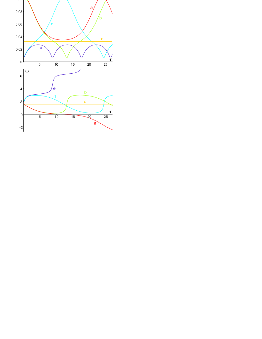
Figure 12.— Planar $y-z$ orbits, solutions of equation (73) in a potential with $\epsilon_{c}=10^{-2},\epsilon_{b}=\epsilon_{c}/2,\varkappa=10^{-4}$, started with $\varpi=\pi/2$ and different $\ell_{0}$: (a) 0.104, (b) 0.103, (c) 0.0322, (d) 0.006, (e) 0.0058. The first two orbits lie close to the separatrix between LATs and pyramids, $\ell_{0+}=0.10392$ (75); the third is the stationary orbit with $\ell_{0}=\ell_{\mathrm{crit}}$; and the last two lie near the separatrix between pyramids and GR-precession-dominated LATs, $\ell_{0-}=0.005845$. Top panel shows the evolution of $\ell(\tau)$, bottom panel shows $\varpi(\tau)$. For pyramid orbits (b–d), the angle $\varpi$ librates around $\pi/2$, and $\ell$ crosses the critical value $\ell_{\mathrm{crit}}$; tube orbits (a,e) have $\varpi$ monotonically circulating, and $\ell$ is always above or below $\ell_{\mathrm{crit}}$.

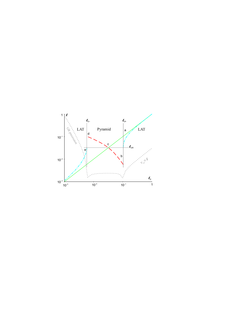
Figure 13.— Minimum and maximum values of $\ell$ for a series of orbits with initial conditions $\ell=\ell_{0}$, $\omega=\pi/2$, $\ell_{z}=0$, $\Omega=\pi/2$. Potential parameters are $\epsilon_{c}=10^{-2},\epsilon_{b}=\epsilon_{c}/2,\varkappa=10^{-4}$. The straight line is $\ell=\ell_{0}$; dashed line is the extremum for pyramids, equation (77). These two curves intersect at $\ell_{\mathrm{crit}}$ (equation 70), where they exchange roles. For $\ell>\ell_{0+}$ and $\ell<\ell_{0-}$ (equation 75) the orbit is a tube, and the minimum (or maximum) is given by equation (76). Dotted grey line shows the leading frequency of $\varpi$ oscillations, $\nu_{\varpi}\times 10^{-2}$; for high-$\ell$ orbits $\nu_{\varpi}\approx 3\ell$, for orbits dominated by GR precession $\nu_{\varpi}\approx 2\varkappa/\ell^{2}$. Letters denote the position of orbits shown in Figure 12.

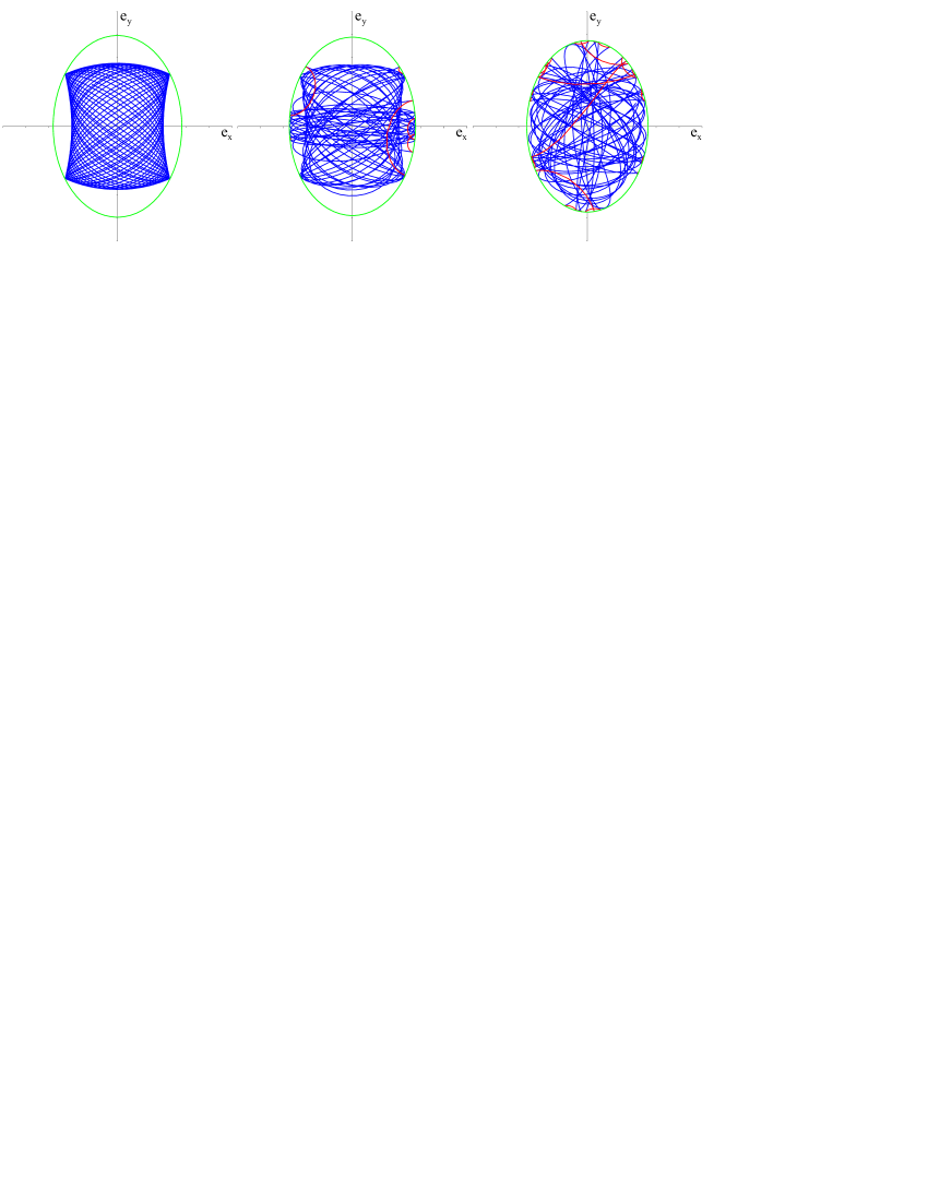
Figure 14.— Three pyramid orbits with the same initial conditions ($\ell=0.05,\ell_{z}=0.02,\varpi=\Omega=\pi/2;\epsilon_{c}=0.01,\epsilon_{b}=0.005$) and three values of the GR coefficient $\varkappa$ (equation 69b). Left: $\varkappa=0$ (regular); middle: $\varkappa=10^{-6}$ (weakly chaotic); right: $\varkappa=10^{-5}$ (strongly chaotic). The green ellipse marks the maximal extent of the ($e_{x},e_{y}$) vector, equation (79), i.e. $\ell=\ell_{\mathrm{crit}}$, equation (70); red segments correspond to $\ell<\ell_{\mathrm{crit}}$, blue to $\ell>\ell_{\mathrm{crit}}$ and to the nonrelativistic case.

In the case of pyramid orbits that are not restricted to a principal plane, numerical solution of the equations of motion derived from the Hamiltonian (69a) are observed to be generally chaotic, increasingly so as $\varkappa$ is increased (Figure 14). This may be attributed to the “scattering” effect of the GR term $\varkappa/l$ in the Hamiltonian, which causes the vector $(e_{x},e_{y})$ to be deflected by an almost random angle whenever $\ell$ approaches zero. In the limit that the motion is fully chaotic, $H$ remains the only integral of the motion. The following argument suggests that the minimum value of the angular momentum attained in this case should be the same as in equation (77).

Suppose that the Hamiltonian (71) is the only integral that remains. Then the vector ($e_{x},e_{y}$) can lie anywhere inside an ellipse

$$Q(e_{x},e_{y})\equiv\frac{5}{2}\left[\epsilon_{c}e_{x}^{2}+(\epsilon_{c}-\epsilon_{b})e_{y}^{2}\right]\leq Q_{\mathrm{max}}\,,$$ (79)

whose boundary is given by

$$Q_{\mathrm{max}}=\frac{5}{2}\epsilon_{c}-H-P_{\mathrm{min}}.$$ (80)

This ellipse defines the base of the “pyramid” (which now rather resembles a cone). As in the planar case, the maximum and minimum values of $\ell$ are attained not on the boundary of this ellipse (i.e. the corners in the Newtonian case), but at $e_{x}=e_{y}=0$, where $Q=0$ and $P$ attains its maximum. These values are given by the roots of the equation $P(\ell)=\frac{5}{2}\epsilon_{c}-H$, or

$$3\ell^{3}-(5\epsilon_{c}-2H)\ell+6\ell_{c}^{3}=0\,.$$ (81)

The two positive roots of this cubic equation are given by

$$\ell_{\mathrm{min,max}} = \frac{2}{3}\sqrt{5\epsilon_{c}-2H}\,\sin\left(\frac{\pi}{6}\pm\phi\right)\;,$$ (82)

$$\phi = \frac{1}{3}\arccos\left(\frac{9\varkappa}{(5\epsilon_{c}-2H)^{3/2}}\right)\;.$$

The plus sign in the argument of the sine function gives $\ell_{\mathrm{max}}$ while the minus sign gives $\ell_{\mathrm{min}}$. These two values are linked by a simple relation:

$$\ell_{\mathrm{min}}=\frac{\ell_{\mathrm{max}}}{2}\left(\sqrt{1+8\varkappa\ell_{\mathrm{max}}^{3}/3}-1\right)\approx\frac{2}{3}\frac{\varkappa}{\ell_{\mathrm{max}}^{2}}\,,$$ (83)

where the latter approximate equality holds for $\varkappa\ll\ell_{\mathrm{max}}^{3}$. In the same approximation

$$\ell_{\mathrm{min}}\approx\frac{2\varkappa}{5\epsilon_{c}-2H}\;,\quad\ell_{\mathrm{max}}^{2}\approx\frac{5\epsilon_{c}-2H}{3}\,.$$ (84)

Equation (77) for planar pyramids is a special case of this relation where $\ell_{0}=\ell_{\mathrm{max}}$.

The ellipse (79) serves as a “reflection boundary” for trajectories that come below $\ell\approx\ell_{\mathrm{crit}}$. If this happens, the vector ($e_{x},e_{y}$) is observed to be quickly “scattered” by an almost random angle (Figure 14, right, denoted by the red segments), similar to the rapid change in $\varpi$ that occurs in the planar case (Figure 12). Roughly speaking, all pyramid orbits and some tube orbits (those that may attain $\ell\leq\ell_{\mathrm{crit}}$) will be chaotic.

The distinction between pyramids and chaotic tubes is in the radius of this ellipse: pyramids by definition have a fixed sign of $e_{z}$, or $e_{x}^{2}+e_{y}^{2}<1$, which means that the ellipse (79) should not touch the circle $e_{x}^{2}+e_{y}^{2}=1$. Hence pyramids have $Q\leq\frac{5}{2}(\epsilon_{c}-\epsilon_{b})$, and

$$\frac{5}{2}\epsilon_{b}-P_{\mathrm{min}}\leq H\leq\frac{5}{2}\epsilon_{c}-P_{\mathrm{min}}.$$ (85)

This condition is different from the one described in §4 even in the case $\varkappa=0=P_{\mathrm{min}}$, since now pyramids do not coexist with LAT orbits.

The condition for LATs to be chaotic (i.e. to pass through $\ell_{\mathrm{crit}})$ is $P_{\mathrm{min}}+Q_{\mathrm{max}}\leq\frac{5}{2}\epsilon_{c}-H$. For LATs the ellipse (79) always intersects the unit circle, so this condition can be satisfied for $-P_{\mathrm{min}}\leq H\leq\frac{5}{2}\epsilon_{b}-P_{\mathrm{min}}$. However, this is a necessary but not sufficient condition for a chaotic LAT: some orbits from this range do not attain $\ell<\ell_{\mathrm{crit}}$ because of the existence of another integral of motion besides $H$ (that is, they are regular).

Finally, we consider the character of the motion when the precession is dominated by GR, as would be the case very near the BH. This is equivalent to staying on the left branch of $P(\ell)$, with $\ell_{\mathrm{min,max}}\ll\ell_{0-}<\ell_{\mathrm{crit}}$ (75). In this limit there is a second short time scale in addition to the radial period, the time for GR precession. This situation is similar to the high-$\ell$ case (§ 4.4), in the sense that we can carry out a second averaging over $\varpi$ and obtain the equations that describe the precession of an annulus due to the triaxial torques. The orbits in this case are again short- or long-axis tubes. The only difference from § 4.4 is that we have to add the term $-\varkappa/\ell$ to the averaged Hamiltonian (41), but since $\ell$ is constant in this approximation, the equations of motion for $\ell_{z},\Omega$ do not change. These very-low-$\ell$ regular tube orbits can be easily captured by the BH, however their number is very small and we do not consider them when computing the total capture rate.

We argue in §8 that the conservation of $\ell$ for orbits in this limit can have important consequences for resonant relaxation.

7.3. Capture of orbits by the BH in the case of GR

The inclusion of general relativistic precession has the effect of limiting the maximum eccentricity achievable by a pyramid orbit. However, if $\ell_{\mathrm{min}}\leq\ell_{\bullet}$, an orbit can still come close enough to the BH to be disrupted or captured. Introducing the quantity $w\equiv\ell_{\mathrm{min}}/\ell_{\bullet}$, we can write

$$w\equiv\frac{\ell_{\mathrm{min}}}{\ell_{\bullet}}\simeq\frac{1}{\ell_{\bullet}}\frac{2\varkappa}{5\epsilon_{c}-2H}\gtrsim\frac{3}{5\epsilon_{c}}\frac{\nu_{r}}{\nu_{p}}\frac{\ell_{\bullet}}{\Theta}\,,$$ (86)

where we used (68, 69b) and set $H=0$ as a lower limit for pyramid orbits (orbits with the smallest $H$ have the largest $\ell_{\mathrm{max}}$ and the smallest $\ell_{\mathrm{min}}$). Comparison with equation (60), with $W\leq(15\epsilon_{c})^{2}$, shows that

$$w\approx\frac{3\pi}{\Theta}\,q^{-1}.$$ (87)

Roughly speaking, the condition that stars be captured ($w<1$) is equivalent to the statement that the loss cone is full ($q>1$). This is not a simple coincidence: a full loss cone implies that for low-$\ell$ orbits the mean change of $\ell$ during one radial period ($\sim\nu_{0}\ell_{0}\,\nu_{p}/\nu_{r}$) is of order $\ell_{\bullet}$, while the condition $w=1$ requires that for the lowest allowable $\ell$, the GR precession rate (68) is comparable to the radial frequency. These two conditions are roughly equivalent.

We can express this necessary condition for capture in terms of more physically relevant quantities. Writing equation (14a) as

$$\frac{\nu_{p}}{\nu_{r}}\approx\frac{1}{2}\frac{M(a)}{{M_{\bullet}}},$$ (88)

and approximating $r_{\mathrm{infl}}$ of equation (2) as

$$r_{\mathrm{infl}}\approx\frac{G{M_{\bullet}}}{\sigma^{2}}\equiv r_{0}$$ (89)

with $\sigma$ the one-dimensional stellar velocity dispersion at $r=r_{\mathrm{infl}}$, the condition $w\leq 1$ becomes

$$\frac{1}{\epsilon_{c}\sqrt{\Theta}}\frac{\sigma}{c}\left(\frac{a}{r_{0}}\right)^{\gamma-7/2}\lesssim 1.$$ (90)

The Milky Way BH constitutes one extreme of the BH mass distribution. Writing $\Theta\approx 10$ (solar-mass main sequence stars), $\sigma\approx 10^{2}$ km s^-1, and $\gamma=3/2$ gives

$$\epsilon_{c}^{1/2}\frac{a}{r_{0}}\gtrsim 10^{-2}$$ (91)

e.g. for $a=0.1r_{0}\approx 0.3$ pc, $\epsilon_{c}\gtrsim 10^{-3}$ is required for stars to be captured. This is a reasonable degree of triaxiality for the Galactic center.

At the other mass extreme, we consider the galaxy M87, for which $\sigma\approx 350$ km s^-1 and $\Theta\approx 3$. Setting $\gamma=0.5$, corresponding to a low-density core, we find

$$\epsilon_{c}^{1/3}\frac{a}{r_{0}}\gtrsim 10^{-1}.$$ (92)

A dimensionless triaxiality of order unity is reasonable for a giant elliptical galaxy.

In § 9 we estimate the loss rate using the expression (64b) for the full loss cone rate, with the modification that the fraction of time $\mu$ an orbit spends inside the loss cone is now given not by (52), but by

$$\mu\approx\frac{\ell_{\bullet}^{2}-\ell_{\mathrm{min}}^{2}}{\ell_{0}^{2}-\ell_{\mathrm{min}}^{2}}.$$ (93)

This relation implies that the instantaneous value of $\ell^{2}$ is distributed uniformly in the range $[\ell_{\mathrm{min}}^{2}..\ell_{\mathrm{max}}^{2}]$. This is a good approximation for chaotic pyramid orbits and a reasonable (within a factor of few) approximation for chaotic LATs (and also for regular orbits).

In the next section we point out the importance of the angular momentum limit for the rate of gravitational wave events due to inspiral of compact stellar remnants.

8. Connection with “resonant relaxation”

Resonant relaxation (RR) is a phenomenon that arises in stellar systems exhibiting certain regularities in the motion (Rauch & Tremaine, 1996; Hopman & Alexander, 2006a). Due to the discreteness of the stellar distribution, torques acting on a test star from all other stars do not cancel exactly, and there is a residual torque that produces a change in the angular momentum:

$$\left|\frac{d{\bf L}}{dt}\right|\approx\sqrt{N}\,\frac{Gm}{a}=L_{c}\,\frac{\sqrt{N}\,m}{M_{\bullet}}2\pi P^{-1}$$ (94)

(here $m$ is the stellar mass, $P=2\pi/\mu_{r}$ is the radial period, $L_{c}\equiv\sqrt{GM_{\bullet}a}$ is the angular momentum of a circular orbit with radius $a$, and $N$ is roughly the number of stars within a sphere of radius $a$). In a non-resonant system this net torque changes the direction randomly after each radial period, but in the case of near-Keplerian motion, for example, orbits remain almost the same for many radial periods, so the change of angular momentum produced by this torque continues in the same direction for a much longer time, the so-called coherence time $t_{\mathrm{coh}}$, until the orientation of either the test star’s orbit or the other stars’ orbits change significantly. If this decoherence is due to precession of stars in their mean field, then

$$t_{\mathrm{coh}}\approx t_{\mathrm{M}}\equiv\nu_{p}^{-1}\approx\frac{{M_{\bullet}}}{m}\frac{P}{N}$$ (95)

where the relevant precession time is that for an orbit of average eccentricity.

The total change of ${\bf L}$ during $t_{\mathrm{coh}}$ is

$$(\Delta L)_{\mathrm{coh}}\approx\sqrt{N}\,\frac{Gm}{a}\,t_{\mathrm{coh}}\approx\frac{L_{c}}{\sqrt{N}}.$$ (96)

On timescales longer than $t_{\mathrm{coh}}$ the angular momentum experiences a random walk with step size $(\Delta L)_{\mathrm{coh}}$ and time step $t_{\mathrm{coh}}$. The relaxation time is defined as the time required for an orbit to change its angular momentum by $L_{c}$, and hence it is given by

$$t_{RR,s}\approx\left(\frac{L_{c}}{\Delta L}\right)^{2}\,t_{\mathrm{coh}}\approx P\,\frac{M_{\bullet}}{m}.$$ (97)

The above argument describes “scalar” resonant relaxation, in which both the magnitude and direction of $\mathbf{L}$ can change. On longer timescales, precessing orbits fill annuli, which also exert mutual torques; however, since these torques are perpendicular to $\mathbf{L}$, they may change only the direction, not the magnitude of $\mathbf{L}$. This effect is dubbed vector resonant relaxation (VRR), and its coherence time is given by the time required for orbital planes to change. In a spherically symmetric system the only mechanism that changes orbital planes is the relaxation itself. Hence for VRR the coherence time is given by setting $\left|d{\bf L}/dt\right|=L_{c}/t_{\mathrm{coh}}$ in equation (94):

$$t_{\mathrm{coh}}\equiv t_{\Omega,\mathrm{VRR}}\approx\frac{{M_{\bullet}}}{m}\frac{P}{\sqrt{N}}\approx\sqrt{N}t_{\mathrm{M}}$$ (98)

and the relaxation time, equation (97), becomes

$$t_{RR,v}\approx t_{\Omega,\mathrm{VRR}}\approx P\,\frac{M_{\bullet}}{m\sqrt{N}}$$ (99)

which is $\sim\sqrt{N}$ times shorter than the scalar relaxation time.

We begin by comparing RR timescales with timescales for orbital change due to a triaxial background potential. Consider a star on a (regular) pyramid orbit confined to the $x-z$ plane. It experiences periodic changes of angular momentum $\ell\equiv L/L_{c}$ with frequency $\lesssim\nu_{x0}\nu_{p}$ (22) and amplitude $\ell_{x0}\lesssim\nu_{x0}/3$ (24). Hence, the typical rate of change of angular momentum is

$$\frac{dL}{dt}\approx L_{c}\,\nu_{x0}^{2}\nu_{p}/3\approx L_{c}\,5\epsilon_{c}\frac{Nm}{M_{\bullet}}2\pi P^{-1}\,.$$ (100)

Comparison with (94) shows that the rate of change of angular momentum due to unbalanced torques from the other stars (RR) is greater than the rate of regular precession if $\epsilon\sqrt{N}\lesssim 1$. However, the coherence time for RR is a typical precession time of stars in the cluster, $\nu_{p}^{-1}$, whereas pyramids change angular momentum on a longer timescale $(\nu_{p}\sqrt{15\epsilon})^{-1}$. On the other hand, in the case of RR the angular momentum continues to change in a random-walk manner on timescale longer than $t_{\mathrm{coh}}$, while in the case of precession in triaxial potential its variation is bounded.

Next we consider VRR, which corresponds to changes in orbital planes defined by the angles $\Omega$ and $i=\arccos(\ell_{z}/\ell)$. The frequency of orbital plane precession in a triaxial potential, $\nu_{\Omega}$, is $\sim\nu_{p}\sqrt{\epsilon}$ for low-$\ell$ orbits (pyramids and saucers) and even lower for other orbits (Figure 2). The corresponding timescale may be written as

$$t_{\Omega,\mathrm{triax}}\ \gtrsim\frac{{M_{\bullet}}}{m}\frac{P}{N\sqrt{\epsilon}}.$$ (101)

Comparison with the VRR timescale (99) shows that $t_{RR,v}/t_{\Omega,\mathrm{triax}}\lesssim\sqrt{N\epsilon}$. For the Milky Way, these two timescales are roughly equal at $a\sim 0.5$ pc (Figure 15). For sufficiently large $N$ the regular precession due to triaxial torques goes on faster than the relaxation, so the coherence time for VRR is now defined by orbit precession, and the relaxation time itself becomes even longer. On the other hand, for small enough $N$ the VRR destroys orientation of orbital planes before they are substantially affected by triaxial torques. It seems that VRR in triaxial (or even axisymmetric) systems can be suppressed by regular orbit precession; we defer the detailed analysis of relaxation for a future study.

So far we have considered the torques arising under RR as being independent of the torques due to the elongated star cluster. Suppose instead that we identify the $\sqrt{N}$ torques that drive RR with the torques due to the triaxial distortion. The justification is as follows: During the coherent RR phase, the gravitational potential from $N$ orbit-averaged stars can be represented in terms of a multipole expansion. If the lowest-order nonspherical terms in that expansion happen to coincide with the potential generated by a uniform-density triaxial cluster, the behavior of orbits in the coherent RR regime would be identical to what was derived above for orbits in a triaxial nucleus. We stress that this is a contrived model; in general, an expansion of the orbit-averaged potential of $N$ stars will contain nonzero dipole, octupole etc. terms that depend in some complicated way on radius. Nevertheless the comparison seems worth making since (as we argue below) there is one important feature of the motion that should depend only weakly on the details of the potential decomposition.

Equating the torques due to RR

$$T_{\mathrm{RR}}\approx\sqrt{N}\frac{Gm}{r}$$ (102)

with those due to a triaxial cluster,

$$T_{\mathrm{triax}}\approx\epsilon\frac{GNm}{r}$$ (103)

our ansatz becomes

$$\epsilon\approx N^{-1/2}.$$ (104)

As shown above (§7), GR sets a lower limit to the angular momentum of a pyramid orbit (equation 78):

$$\ell_{\mathrm{min}}\approx\frac{\varkappa}{\ell_{0}^{2}}\approx\frac{\kappa}{\epsilon}\approx\frac{r_{\mathrm{Schw}}}{a}\frac{{M_{\bullet}}}{M(a)}\sqrt{N};$$ (105)

the third term comes from setting $\ell_{0}\approx\ell_{\mathrm{max}}\approx\sqrt{\epsilon}$, the maximum value for a pyramid orbit, while the fourth term uses our ansatz (104) and the definition (69b) of $\varkappa$. Expressed in terms of eccentricity,

$$1-e_{\mathrm{max}}\approx\left(\frac{r_{\mathrm{Schw}}}{a}\right)^{2}\left(\frac{{M_{\bullet}}}{m}\right)^{2}\frac{1}{N(a)}.$$ (106)

There is another way to motivate this result that does not depend on a detailed knowledge of the behavior of pyramid orbits. If we require that the GR precession time:

$$\nu_{\mathrm{GR}}^{-1}\approx\frac{\ell^{2}}{\varkappa}\nu_{p}^{-1}$$ (107)

(eq. 68) be shorter than the time

$$\ell\left|\frac{d\ell}{dt}\right|^{-1}\approx\frac{\ell}{\epsilon}\nu_{p}^{-1}$$ (108)

for torques to change $\ell$ by of order itself, then

$$\ell\lesssim\frac{\varkappa}{\epsilon}\approx\sqrt{N}\varkappa\approx\frac{r_{\mathrm{Schw}}}{a}\frac{{M_{\bullet}}}{M(a)}\sqrt{N}$$ (109)

as above. In other words, when $\ell\lesssim\ell_{\mathrm{min}}$, GR precession is so rapid that the $\sqrt{N}$ torques are unable to change the angular momentum significantly over one precessional period.

In order for this limiting angular momentum to be relevant to RR, the timescale for changes in the background potential should be long compared with the time over which an orbit with $\ell\approx\ell_{\mathrm{min}}$ appreciably changes its angular momentum. As just shown, the latter timescale is

$$t_{\mathrm{GR}}\equiv\nu_{\mathrm{GR}}^{-1}\approx\frac{\ell^{2}}{\varkappa}\nu_{p}^{-1}\approx\varkappa N\nu_{p}^{-1}.$$ (110)

The former timescale is the coherence time for VRR, equation (98):

$$t_{\Omega}\approx\frac{{M_{\bullet}}}{m}\frac{P}{\sqrt{N}}.$$ (111)

The condition $t_{\Omega}\gg t_{\mathrm{GR}}$ is then

$$\frac{{M_{\bullet}}}{m}\frac{P}{\sqrt{N}}\gg\varkappa N\nu_{p}^{-1}$$ (112)

or

$$\frac{a}{r_{\mathrm{Schw}}}\sqrt{N}\gg\frac{{M_{\bullet}}}{m}.$$ (113)

Applying this to the center of the Milky Way, the condition becomes

$$\frac{a}{\mathrm{mpc}}\sqrt{N(a)}\gg 10^{2}$$ (114)

which is likely to be satisfied beyond a few mpc from SgrA^∗.

On timescales longer than $\sim t_{\mathrm{coh}}$, the torques driving RR will change direction. This is roughly equivalent in our simple model to changing the orientation of the triaxial ellipsoid, or to changing $\ell_{0}$ at fixed $\ell$. Such changes might induce an orbit to evolve to values of $\ell$ lower than $\ell_{\mathrm{min}}$, by advancing down the narrow “neck” in the lower left portion of Figure 13. However such evolution would be disfavored, for two reasons: (1) it would require a series of correlated changes in the background potential, increasingly so as $\ell$ became small; (2) as $\ell$ decreased and $\nu_{\mathrm{GR}}$ increased, changes in the background potential would occur on timescales progressively longer than the GR precession time, and adiabatic invariance would tend to preserve $\ell$ (§4.4). These predictions can in principle be tested via direct $N$-body integration of small-$N$ systems including post-Newtonian accelerations (e.g Merritt et al., 2010).

A lower limit to the angular momentum for orbits near a massive BH could have important implications for the rate of gravitational wave events due to extreme-mass-ratio inspirals, or EMRIs (Hils & Bender, 1995). The critical eccentricity at which the orbital evolution of a $10M_{\odot}$ compact object begins to be dominated by gravitational wave emission is

$$1-e_{\mathrm{EMRI}}\approx 10^{-5}\left(\frac{t_{r}}{10^{9}\mathrm{yr}}\right)^{-2/3}\left(\frac{{M_{\bullet}}}{10^{6}M_{\odot}}\right)^{4/3}$$ (115)

with $t_{r}$ the relaxation time (e.g. Amaro-Seoane et al., 2007, eq. (6)). By comparison, equation (106), after substitution of $N(<a)=N_{0}(a/\mathrm{mpc})$ implies

$$1-e_{\mathrm{max}}\approx 2\times 10^{-4}\left(\frac{{M_{\bullet}}}{10^{6}M_{\odot}}\right)^{4}\left(\frac{N_{0}}{100}\right)^{-1}\left(\frac{a}{10\mathrm{mpc}}\right)^{-3}.$$ (116)

9. Estimates for real galaxies

In this section we estimate the fraction and lifetime of pyramid orbits to be expected in the nuclei of real galaxies.

We restrict calculations to the case of “maximal triaxiality,” $\epsilon_{b}=\epsilon_{c}/2$, although we leave the amplitudes of $\epsilon_{b},\epsilon_{c}$ free parameters. We also limit the discussion to orbits within the BH influence radius, $r\lesssim r_{\mathrm{infl}}$, where our analysis is valid and where orbits are typically regular. Beyond $\sim r_{\mathrm{infl}}$, centrophilic (mostly chaotic) orbits still exist and could dominate, e.g., the rate of feeding of a central BH (Merritt & Poon, 2004).

The first set of parameters is chosen to describe the center of the Milky Way. The BH mass is set to $M_{\bullet}=4\times 10^{6}~{}M_{\odot}$ (Ghez et al., 2008; Gillessen et al., 2009a, b). The density of the spherically symmetric stellar cusp is taken to be $\rho_{s}=1.5\times 10^{5}\,M_{\odot}\mathrm{pc}^{-3}\,(r/1\mbox{ pc})^{-\gamma}$ (Schödel et al., 2007), with $\gamma=1.5$ (Schödel et al., 2008); the corresponding BH influence radius is $r_{\mathrm{infl}}\approx 3$ pc. The triaxial component of the potential is highly uncertain; one source would be the nuclear bar with density $\rho_{t}\approx 150\,M_{\odot}\mathrm{pc}^{-3}$ (Rodriguez-Fernandez & Combes, 2008), yielding a triaxiality coefficient at $r=1$ pc of $\epsilon_{c}\approx 10^{-3}$. We also considered a larger value, $\epsilon_{c}=10^{-2}$, which may be justified by some kind of asymmetry on spatial scales closer to $r_{\mathrm{infl}}$ than the bar. In this model, the precession time due to the spherical component of the potential, $2\pi/(3\nu_{p})$ for a circular orbit, is independent of radius and equals $\sim 1.7\times 10^{5}$ yr; the two-body relaxation time is also constant ($5\times 10^{9}$ yr), and timescales for scalar and vector resonant relaxation are given by equation (97), (99) with stellar mass $m=1\,M_{\odot}$.

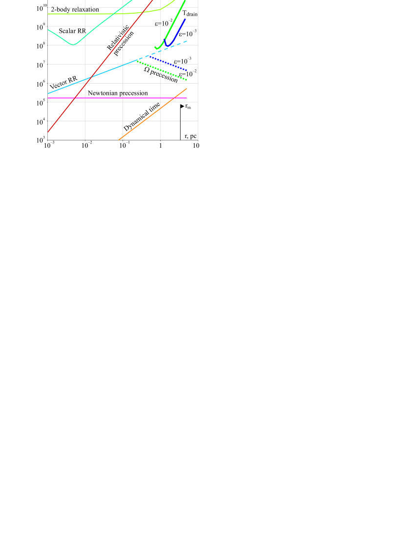
Figure 15.— Various timescales for Milky Way center. Green and blue solid curves are the pyramid draining times (more exact calculation than equation 9) for $\epsilon_{c}=10^{-2}$ and $10^{-3}$; dotted green and blue curves denote typical orbital plane precession timescales $\nu_{\Omega}^{-1}$ for low-$\ell$ orbits ($\ell^{2}\approx\epsilon_{c}(a)$); Newtonian and relativistic precession times are given for circular orbits; other timescales are marked on the plot. Vector resonant relaxation is suppressed when $t_{RR,v}\gtrsim\nu_{\Omega}^{-1}$ (marked by conversion of line into dashed).

The second set of parameters is intended to describe the case of galaxies with more massive BHs, using the so-called $M_{\bullet}-\sigma$ relation in the form

$$M_{\bullet}\approx 1.7\times 10^{8}\,M_{\odot}\,\left(\frac{\sigma}{200\mbox{ km s}^{-1}}\right)^{4.86}$$ (117)

(Ferrarese & Ford, 2005). Combined with the definition of $r_{\mathrm{infl}}\approx GM_{\bullet}/\sigma^{2}$, we get

$$r_{\mathrm{infl}}\approx 13\mbox{ pc}\left(\frac{{M_{\bullet}}}{10^{8}\,M_{\odot}}\right)^{0.59}\;.$$ (118)

The two-body relaxation time evaluated at $r_{\mathrm{infl}}$ (assuming a mean-square stellar mass $m_{\star}=1\,M_{\odot}$ and a Coulomb logarithm $\ln\Lambda=15$) is

$$t_{2br}(r_{\mathrm{infl}}) \approx 2.1\times 10^{13}\mbox{ yr}\left(\frac{\sigma}{200\mbox{ km s}^{-1}}\right)^{7.5}$$ (119a)

$$\approx 9.6\times 10^{12}\mbox{ yr}\left(\frac{{M_{\bullet}}}{10^{8}\,M_{\odot}}\right)^{1.54}$$ (119b)

(Merritt et al., 2007).

We first estimate the radius $r_{\mathrm{crit}}$ that separates the empty ($q<1$) and full loss cone regimes. As noted in the previous section, GR precession prevents a pyramid orbit from reaching arbitrarily low angular momenta; the radius beyond which capture becomes possible is roughly $r_{\mathrm{crit}}$. Using equation (60) with $W=(15\epsilon_{c})^{2}$ (the maximum value for pyramids) and equations (14a), (48), the condition $q=1$ translates to

$$1=\frac{4\pi}{3-\gamma}\frac{\rho_{s}r_{0}^{3}}{M_{\bullet}}\left(\frac{r_{\mathrm{crit}}}{r_{0}}\right)^{3-\gamma}\frac{2\alpha^{\prime}}{3(2-\gamma)}\,\frac{5\pi\,\epsilon_{c}(r_{\mathrm{crit}})}{\sqrt{\Theta r_{\mathrm{Schw}}/r_{\mathrm{crit}}}}$$

If we take $r_{0}$ to be $r_{\mathrm{infl}}$, and $\rho_{s}$ and $\sigma$ as the density and velocity dispersion at this radius, we obtain

$$\frac{r_{\mathrm{crit}}}{r_{\mathrm{infl}}}\approx 0.5\left(\frac{\sigma}{c}\frac{\sqrt{\Theta}}{\epsilon_{c}(r_{0})}\right)^{2/7}.$$ (120)

The radius $r_{\mathrm{crit}}$ typically lies in the range $(0.2-0.7)r_{\mathrm{infl}}$, weakly dependent on the parameters. Since regular pyramid orbits exist only for $a\lesssim r_{\mathrm{infl}}$ (Figure 10), there is evidently a fairly narrow range of radii for which capture of stars from pyramid orbits is possible. However pyramid-like, centrophilic can exist at much larger radii (Poon & Merritt, 2001).

Next we make a rough estimate of the pyramid draining time at $a>r_{\mathrm{crit}}$, using the expression (64b) for the flux in the full loss cone regime, ${\cal F}=\mu/(P\nu_{p})$; $\mu$ (the fraction of phase space occupied by the loss cone) is given by equation (93) with $\ell_{\mathrm{min}}\ll\ell_{\bullet}$, $\ell_{\mathrm{max}}^{2}\approx\frac{5}{3}\epsilon_{c}$ (equation 84):

$$t_{\mathrm{drain}} = \frac{1}{{\cal F}\,\nu_{p}}\approx\frac{5\pi}{3\Theta}\frac{c^{2}}{(GM_{\bullet})^{3/2}}a^{5/2}\epsilon_{c}(a)$$

$$\approx 10^{9}\mbox{ yr}\times\frac{\epsilon_{c}(a)}{\Theta}\left(\frac{M_{\bullet}}{10^{8}\,M_{\odot}}\right)^{-3/2}\left(\frac{a}{1\mbox{ pc}}\right)^{5/2}.$$

A more exact calculation of $t_{\mathrm{drain}}(a)$ for the Milky Way, based on numerical analysis of properties of orbits sampled from the entire phase space, is shown in Figure 15.

Finally, we estimate the total capture rate for all pyramids inside $r_{\mathrm{infl}}$, using $t_{\mathrm{pyr}}\equiv t_{\mathrm{drain}}(r_{\mathrm{infl}})$ as a typical timescale and applying (117, 118, 9):

$$t_{\mathrm{pyr}}\approx 6\times 10^{11}\mbox{ yr}\times\frac{\epsilon_{c}(r_{\mathrm{infl}})}{\Theta}\left(\frac{M_{\bullet}}{10^{8}\,M_{\odot}}\right)^{-0.025}.$$ (122)

The capture rate from pyramids is then

$$\dot{M}_{\mathrm{pyr}}\approx\frac{\epsilon_{c}(r_{\mathrm{infl}})M_{\bullet}}{t_{\mathrm{pyr}}}\approx 1.6\times 10^{-4}\,M_{\odot}\mbox{ yr}^{-1}\Theta\left(\frac{M_{\bullet}}{10^{8}\,M_{\odot}}\right)^{1.025}$$ (123)

For the Milky Way we find $\sim 4\times 10^{-5}\,M_{\odot}$yr^-1 for $\epsilon_{c}=10^{-3}$ and $\sim 10^{-4}\,M_{\odot}$yr^-1 for $\epsilon_{c}=10^{-2}$.

This capture rate should be compared with that due to two-body relaxation, which is estimated to be (Merritt, 2009)

$$\dot{M}_{2br}\approx 0.1\frac{M_{\bullet}}{t_{2br}}\approx 10^{-6}\,M_{\odot}\mbox{yr}^{-1}\times\left(\frac{M_{\bullet}}{10^{8}\,M_{\odot}}\right)^{-0.54}$$ (124)

Thus even for a Milky Way-sized galaxy, the capture rate of pyramids could be comparable with or greater than that due to two-body relaxation. For more massive galaxies this inequality becomes even stronger. However, this is only the initial capture rate – after $\sim t_{\mathrm{pyr}}$, all stars on pyramid orbits would have been consumed, at least in the absence of other mechanisms for repopulating the small-$\ell$ parts of phase space (not necessarily $\ell\lesssim\ell_{\bullet}$, but the much broader region $\ell\lesssim\sqrt{\epsilon_{c}}$ from which draining is effective).

In the most luminous galaxies, like M87, standard mechanisms for relaxation are expected to be ineffective even over Gyr timescales and pyramid orbits once depleted are likely to stay depleted. Setting $\epsilon_{c}=0.1$, $\Theta=3$ and ${M_{\bullet}}=4\times 10^{9}M_{\odot}$ gives for M87 $t_{\mathrm{pyr}}\approx 5$ Gyr and $M_{\mathrm{pyr}}\approx 4\times 10^{8}M_{\odot}$. This could be an effective mechanism for creating a low-density core at the centers of giant elliptical galaxies.

10. Conclusions

We discussed the character of orbits within the radius of influence $r_{\mathrm{infl}}$ of a supermassive BH at the center of a triaxial star cluster. The motion can be described as a perturbation of Keplerian motion; we derive the orbit-averaged equations and explore their solutions both analytically (when the triaxiality is small) and numerically. Orbits are found to be mainly regular in this region. There exist three families of tube orbits; a fourth orbital family, the pyramids, can be described as eccentric Keplerian ellipses that librate in two directions about the short axis of the triaxial figure. At the “corners” of the pyramid, the angular momentum reaches zero, which means that stars on these orbits can be captured by the BH. We derive expressions for the rate at which stars on pyramid orbits would be lost to the BH; there are many similarities with the more standard case of diffusional loss cone refilling, but also some important differences, due to the fact that the approach to the loss cone is deterministic for the pyramids, rather than statistical. The inclusion of general relativistic precession is shown to impose a lower bound on the angular momentum. We argue that a similar lower bound should apply to orbital evolution in the case that the torques are due to resonant relaxation. The rate of consumption of stars from pyramid orbits is likely to be substantially greater than the rate due to two-body relaxation in the most luminous galaxies, although in the absence of mechanisms for orbital repopulation, these high consumption rates would only be maintained until such a time as the pyramid orbits have been drained; however the latter time can be measured in billions of years.

References

- Amaro-Seoane et al. (2007) Amaro-Seoane, P., Gair, J. R., Freitag, M., Miller, M. C., Mandel, I., Cutler, C. J., & Babak, S. 2007, Classical and Quantum Gravity, 24, 113
- Bartko et al. (2010) Bartko, H., et al. 2010, ApJ, 708, 834
- Buchholz et al. (2009) Buchholz, R. M., Schödel, R., & Eckart, A. 2009, A&A, 499, 483
- Cappellari et al. (2007) Cappellari, M., et al. 2007, MNRAS, 379, 418
- Chandrasekhar (1969) Chandrasekhar, S. 1969, The Silliman Foundation Lectures, New Haven: Yale University Press, 1969
- Cohn & Kulsrud (1978) Cohn, H.& Kulsrud, R. 1978, ApJ, 226, 1087
- Do et al. (2009) Do, T., Ghez, A. M., Morris, M. R., Lu, J. R., Matthews, K., Yelda, S., & Larkin, J. 2009, ApJ, 703, 1323
- Eilon, Kupi & Alexander (2009) Eilon, E., Kupi, G. & Alexander, T. 2009, ApJ, 698, 641
- Erwin & Sparke (2002) Erwin, P., & Sparke, L. S. 2002, AJ, 124, 65
- Ferrarese & Ford (2005) Ferrarese, L., & Ford, H. 2005, Space Science Reviews, 116, 523
- Franx et al. (1991) Franx, M., Illingworth, G., & de Zeeuw, T. 1991, ApJ, 383, 112
- Ghez et al. (2008) Ghez, A. et al., ApJ, 689, 1044
- Gillessen et al. (2009a) Gillessen, S. et al. 2009a, ApJ, 692, 1075
- Gillessen et al. (2009b) Gillessen, S. et al. 2009b, ApJ, 707, 114
- Goldstein et al. (2002) Goldstein, H., Poole, C., & Safko, J. 2002, Classical mechanics (3rd ed.) San Francisco: Addison-Wesley
- Hils & Bender (1995) Hils, D., & Bender, P. L. 1995, ApJ, 445, L7
- Hopman & Alexander (2006a) Hopman, C., & Alexander, T. 2006, ApJ, 645, 1152
- Hopman & Alexander (2006b) Hopman, C., & Alexander, T. 2006b, ApJ, 645, L133
- Ivanov (2002) Ivanov, P. B. 2002, MNRAS, 336, 373
- Ivanov, Polnarev & Saha (2005) Ivanov, P. B, Polnarev, A. G. & Saha, P. 2005, MNRAS, 358, 1361
- Lees & Schwarzschild (1992) Lees, J. F., & Schwarzschild, M. 1992, ApJ, 384, 491
- Merritt (2009) Merritt, D. 2009, ApJ, 694, 959
- Merritt et al. (2010) Merritt, D., Alexander, T., Mikkola, S., & Will, C. M. 2010, Phys. Rev. D, 81, 062002
- Merritt et al. (2007) Merritt, D., Mikkola, S., & Szell, A. 2007, ApJ, 671, 53
- Merritt & Milosavljevic (2005) Merritt, D. & Milosavljevic, M. 2005, Living Rev. Rel., 8, 8
- Merritt & Poon (2004) Merritt, D., & Poon, M. Y. 2004, ApJ, 606, 788
- Merritt & Valluri (1999) Merritt, D., & Valluri, M. 1999, AJ, 118, 1177
- Polyachenko, Polyachenko & Shukhman (2007) Polyachenko, E. V., Polyachenko, V. L. & Shukhman, I. G. 2007, MNRAS, 379, 573
- Poon & Merritt (2001) Poon, M. & Merritt, D. 2001, ApJ, 549, 192
- Poon & Merritt (2004) Poon, M. Y., & Merritt, D. 2004, ApJ, 606, 774
- Rauch & Tremaine (1996) Rauch, K. & Tremaine, S. 1996, New Astron., 1, 149
- Richstone (1982) Richstone, D. O. 1982, ApJ, 252, 496
- Rodriguez-Fernandez & Combes (2008) Rodriguez-Fernandez, N. J., Combes, F. 2008, A&A, 489, 115
- Sambhus & Sridhar (2000) Sambhus, N. & Sridhar, S. 2000, ApJ, 542, 143
- Sanders & Verhulst (1985) Sanders, J. A., & Verhulst, F. 1985, Averaging methods in nonlinear dynamical systems. Applied Mathematical Sciences, Vol. 59. Springer-Verlag, New York - Berlin - Heidelberg - Tokyo
- Schödel et al. (2007) Schödel, R. et al. 2007, A&A, 469, 125
- Schödel et al. (2008) Schödel, R., Merritt, D., Eckart, A. 2008, Journal of Physics: Conference Series, 131, 012044
- Schwarzschild (1979) Schwarzschild, M. 1979, ApJ, 232, 236
- Schwarzschild (1982) Schwarzschild, M. 1982, ApJ, 263, 599
- Seth et al. (2008) Seth, A. C., Blum, R. D., Bastian, N., Caldwell, N., & Debattista, V. P. 2008, ApJ, 687, 997
- Shaw et al. (1993) Shaw, M. A., Combes, F., Axon, D. J., & Wright, G. S. 1993, A&A, 273, 31
- Sridhar & Touma (1997) Sridhar, S. & Touma, J. 1997, MNRAS, 287, L1
- Sridhar & Touma (1999) Sridhar, S. & Touma, J. 1999, MNRAS, 303, 483
- Statler et al. (2004) Statler, T. S., Emsellem, E., Peletier, R. F., & Bacon, R. 2004, MNRAS, 353, 1
- Valluri & Merritt (1998) Valluri, M., & Merritt, D. 1998, ApJ, 506, 686
- Wang & Merritt (2004) Wang, J., & Merritt, D. 2004, ApJ, 600, 149
- Weinberg (1972) Weinberg, S. 1972, Gravitation and Cosmology: Principles and Applications of the General Theory of Relativity (Wiley)
- de Zeeuw (1985) de Zeeuw, T. 1985, MNRAS, 216, 273