Recovery of sparsest signals via $\ell^{q}$-minimization

Abstract.

In this paper, it is proved that every $s$-sparse vector ${\bf x}\in{\mathbb{R}}^{n}$ can be exactly recovered from the measurement vector ${\bf z}={\bf A}{\bf x}\in{\mathbb{R}}^{m}$ via some $\ell^{q}$-minimization with $0<q\leq 1$, as soon as each $s$-sparse vector ${\bf x}\in{\mathbb{R}}^{n}$ is uniquely determined by the measurement ${\bf z}$.

1. Introduction and Main Results

Define the norm $\|{\bf x}\|_{q},0\leq q\leq\infty$, of a vector ${\bf x}=(x_{1},\ldots,x_{n})^{T}\in{\mathbb{R}}^{n}$ by the number of its nonzero components when $q=0$, the quantity $(|x_{1}|^{q}+\cdots+|x_{n}|^{q})^{1/q}$ when $0<q<\infty$, and the maximum absolute value $\max(|x_{1}|,\ldots,|x_{n}|)$ of its components when $q=\infty$. We say that a vector ${\bf x}\in{\mathbb{R}}^{n}$ is $s$-sparse if $\|{\bf x}\|_{0}\leq s$, i.e., the number of its nonzero components is less than or equal to $s$.

In this paper, we consider the problem of compressive sensing in finding $s$-sparse solutions ${\bf x}\in{\mathbb{R}}^{n}$ to the linear system

(1.1) $${\bf A}{\bf x}={\bf z}$$

via solving the $\ell^{q}$-minimization problem:

(1.2) $$\min\|{\bf y}\|_{q}\quad{\rm subject\ to}\ {\bf A}{\bf y}={\bf z}$$

where $0<q\leq 1$, $2\leq 2s\leq m\leq n$, ${\bf A}$ is an $m\times n$ matrix, and ${\bf z}\in{\mathbb{R}}^{m}$ is the observation data ([1, 5, 7, 9, 12, 14]).

One of the basic questions about finding $s$-sparse solutions to the linear system (1.1) is under what circumstances the linear system (1.1) has a unique solution in $\Sigma_{s}$, the set of all $s$-sparse vectors.

Proposition 1.1.

([12, 15]) Let $2s\leq m\leq n$ and ${\bf A}$ be an $m\times n$ matrix. Then the following statements are equivalent:

• The measurement ${\bf A}{\bf x}$ uniquely determines each $s$-sparse vector ${\bf x}$.

• There is a decoder $\Delta:{\mathbb{R}}^{m}\longmapsto{\mathbb{R}}^{n}$ such that $\Delta({\bf A}{\bf x})={\bf x}$ for all ${\bf x}\in\Sigma_{s}$.

• The only $2s$-sparse vector ${\bf y}$ that satisfies ${\bf A}{\bf y}={\bf 0}$ is the zero vector.

• There exist positive constants $\alpha_{2s}$ and $\beta_{2s}$ such that

  (1.3) $$\alpha_{2s}\|{\bf x}\|_{2}\leq\|{\bf A}{\bf x}\|_{2}\leq\beta_{2s}\|{\bf x}\|_{2}\quad\ {\rm for\ all}\ {\bf x}\in\Sigma_{2s}.$$

The first contribution of this paper is to provide another equivalent statement:

• There exists $0<q\leq 1$ such that the decoder $\Delta:{\mathbb{R}}^{m}\longmapsto{\mathbb{R}}^{n}$ defined by

  (1.4) $$\Delta({\bf z}):={\rm argmin}_{{\bf Ay}={\bf z}}\|{\bf y}\|_{q}$$

  satisfies $\Delta({\bf A}{\bf x})={\bf x}$ for all ${\bf x}\in\Sigma_{s}$.

The implication from (v) to (ii) is obvious. Hence it suffices to prove the implication from (iv) to (v). For this, we recall the restricted isometry property of order $s$ for an $m\times n$ matrix ${\bf A}$, i.e., there exists a positive constant $\delta\in(0,1)$ such that

(1.5) $$(1-\delta)\|{\bf x}\|_{2}^{2}\leq\|{\bf A}{\bf x}\|_{2}^{2}\leq(1+\delta)\|{\bf x}\|_{2}^{2}\quad\ {\rm for\ all}\ {\bf x}\in\Sigma_{s}.$$

The smallest positive constant $\delta$ that satisfies (1.5), to be denoted by $\delta_{s}({\bf A})$, is known as the restricted isometry constant [5, 7]. Notice that given a matrix ${\bf A}$ that satisfies (1.3), its rescaled matrix ${\bf B}:=\sqrt{2/(\alpha_{2s}^{2}+\beta_{2s}^{2})}{\bf A}$ has the restricted isometry property of order $2s$ and its restricted isometry constant is given by $(\beta_{2s}^{2}-\alpha_{2s}^{2})/(\alpha_{2s}^{2}+\beta_{2s}^{2})$. Therefore the implication from (iv) to (v) further reduces to establishing the following result:

Theorem 1.2.

Let integers $m,n$ and $s$ satisfy $2s\leq m\leq n$. If ${\bf A}$ is an $m\times n$ matrix with $\delta_{2s}({\bf A})\in(0,1)$, then there exists $0<q\leq 1$ such that any $s$-sparse vector ${\bf x}$ can be exactly recovered by solving the $\ell^{q}$-minimization problem:

(1.6) $$\min\|{\bf y}\|_{q}\quad{\rm subject\ to}\ \ {\bf A}{\bf y}={\bf A}{\bf x}.$$

The above existence theorem about $\ell^{q}$-minimization is established in [17] and [9] under a stronger assumption that $\delta_{2s+2}({\bf A})\in(0,1)$ and $\delta_{2s+1}({\bf A})\in(0,1)$ respectively, as it is obvious that $\delta_{2s}({\bf A})\leq\delta_{2s+1}({\bf A})\leq\delta_{2s+2}({\bf A})$ for any $m\times n$ matrix ${\bf A}$.

Given integers $s,m$ and $n$ satisfying $2s\leq m\leq n$ and an $m\times n$ matrix ${\bf A}$, define

(1.7) $$q_{s}({\bf A}) := \sup\big{\{}q\in[0,1]\big{|}\ {\rm any\ vector}\ {\bf x}\in\Sigma_{s}\ {\rm can\ be\ exactly\ recovered}$$

$${\rm by\ solving\ the}\ \ell^{q}-{\rm minimization\ problem}\ \eqref{section1.eq5}\big{\}}.$$

Then $q_{s}({\bf A})>0$ whenever $\delta_{2s}({\bf A})<1$ by Theorem 1.2. It is also known that any $s$-sparse vector ${\bf x}\in{\mathbb{R}}^{n}$ can be exactly recovered by solving the $\ell^{q}$-minimization problem (1.6) whenever $q<q_{s}({\bf A})$ [18]. This establishes the equivalence among different $q\in[0,q_{s}({\bf A}))$ in recovering $s$-sparse solutions via solving the $\ell^{q}$-minimization problem (1.6). Hence in order to recover sparsest vector ${\bf x}$ from the measurement ${\bf A}{\bf x}$, one may solve the $\ell^{q}$-minimization problem (1.6) for some $0<q\leq 1$ rather than the $\ell^{0}$-minimization problem. Empirical evidence ([9, 22, 23]) strongly indicates that solving the $\ell^{q}$-minimization problem with $0<q\leq 1$ takes much less time than with $q=0$.

The $\ell^{0}$-minimization problem is a combinatorial optimization problem and NP-hard to solve [20], while on the other hand the $\ell^{1}$-minimization is convex and polynomial-time solvable [2]. To guarantee the equivalence between the $\ell^{0}$ and $\ell^{1}$-minimization problems (1.6) in finding the sparse vector ${\bf x}$ from its measurement ${\bf A}{\bf x}$, one needs to meet various requirements on the matrix ${\bf A}$, for instance, $\delta_{s}({\bf A})+\delta_{2s}({\bf A})+\delta_{3s}({\bf A})<1$ in [6], $\delta_{3s}({\bf A})+3\delta_{4s}({\bf A})<2$ in [5], and $\delta_{2s}({\bf A})<1/3\approx 0.3333,\sqrt{2}-1\approx 0.4142,2/(3+\sqrt{2})\approx 0.4531,2/(2+\sqrt{5})\approx 0.4731,4/(6+\sqrt{6})\approx 0.4734$ in [12, 4, 17, 3, 16] respectively. Many random matrices with i.d.d. entries satisfy those requirement to guarantee the equivalence [7], but lots of deterministic matrices do not. In particular, matrices ${\bf A}_{\epsilon}$ are constructed in [13] for any $\epsilon>0$ such that $\delta_{2s}({\bf A}_{\epsilon})<1/\sqrt{2}+\epsilon$ and that it fails on the recovery of some $s$-sparse vectors ${\bf x}$ by solving the $\ell^{1}$-minimization problem (1.6) with ${\bf A}$ replaced by ${\bf A}_{\epsilon}$.

The $\ell^{q}$-minimization problem (1.6) with $0<q<1$ is more difficult to solve than the $\ell^{1}$-minimization problem due to the nonconvexity and nonsmoothness. In fact, it is NP-hard to find a global minimizer in general but polynomial-time doable to find local minimizer [19]. Various algorithms have been developed to solve the $\ell^{q}$-minimization problem (1.6), see for instance [8, 11, 14, 17, 21].

For any $\delta\in(0,1)$, define

(1.8) $$q_{\max}(\delta;m,n,s):=\inf_{\delta_{2s}({\bf A})\leq\delta}q_{s}({\bf A}).$$

Then given any positive number $q<q_{\max}(\delta;m,n,s)$ and any $m\times n$ matrix ${\bf A}$ with $\delta_{2s}({\bf A})\leq\delta$, any vector ${\bf x}\in\Sigma_{s}$ can be exactly recovered by solving the $\ell^{q}$-minimization problem (1.6). For any $0<q\leq 1$ and sufficiently small $\epsilon$, matrices ${\bf A}_{\epsilon}$ of size $(n-1)\times n$ are constructed in [13] such that $\delta_{2s}({\bf A}_{q,\epsilon})<\frac{\eta_{q}}{2-q-\eta_{q}}+\epsilon$ and there is an $s$-sparse vector which cannot be recovered exactly by solving the $\ell^{q}$-minimization problem (1.6) with ${\bf A}$ replaced by ${\bf A}_{q,\epsilon}$, where $\eta_{q}$ is the unique positive solution to $\eta_{q}^{2/q}+1=2(1-\eta_{q})/q$. The above construction of matrices for which the $\ell^{q}$-minimization fails to recover $s$-sparse vectors, together with the asymptotic estimate $\eta_{q}=1-qx_{0}+o(q)$ as $q\to 0$, gives that

(1.9) $$\limsup_{\delta\to 1-}\frac{q_{\max}(\delta;n-1,n,s)}{1-\delta}\leq\lim_{q\to 0+}\frac{q(2-q-\eta_{q})}{2-q-2\eta_{q}}=\frac{1}{2x_{0}-1}\approx 3.5911,$$

where $x_{0}$ is the unique positive solution of the equation $e^{-2x}=2x-1$. The second contribution of this paper is a lower bound estimate for $q_{\max}(\delta;m,n,s)$ as $\delta\to 1-$.

Theorem 1.3.

Let $q_{\max}(\delta;m,n,s)$ be defined as in (1.8). Then

(1.10) $$\liminf_{\delta\to 1-}\frac{q_{\max}(\delta;m,n,s)}{1-\delta}\geq\frac{e}{4}\approx 0.6796.$$

Denote by ${\bf v}_{S}$ the vector which equals to ${\bf v}\in{\mathbb{R}}^{n}$ on $S$ and vanishes on the complement $S^{c}$ where $S\subset\{1,\ldots,n\}$. We say that an $m\times n$ matrix ${\bf A}$ has the null space property of order $s$ in $\ell^{q}$ if there exists a positive constant $\gamma$ such that

(1.11) $$\|{\bf h}_{S}\|_{q}\leq\gamma\|{\bf h}_{S^{c}}\|_{q}$$

hold for all ${\bf h}$ satisfying ${\bf A}{\bf h}={\bf 0}$ and all sets $S$ with its cardinality $\#S$ less than or equal to $s$ ([12]). The minimal constant $\gamma$ in (1.11) is known as the null space constant.

For $0<q\leq 1$ and $\delta\in(0,1)$, define

(1.12) $$a(q,\delta) := \inf_{0<r_{0}<1}\max\Big{\{}\frac{1+r_{0}\delta}{(1+r_{0}^{q}\delta^{q})^{1/q}},\sup_{\sqrt{2}(1-r_{0})\delta/2\leq y\leq 1}\frac{2y}{\big{(}1+2^{-q/2}y^{2+q}\big{)}^{1/q}},$$

$$\quad\sup_{\sqrt{2}(1-r_{0})\delta/2\leq y\leq 1}\frac{3y}{\big{(}1+y\big{)}^{1/q}},\ \sup_{1\leq y}\frac{2y}{\big{(}1+y\big{)}^{1/q}}\Big{\}}.$$

The third contribution of this paper is the following result about the null space property of an $m\times n$ matrix.

Theorem 1.4.

Let $q$ be a positive number in $(0,1]$, integers $m,n$ and $s$ satisfy $2s\leq m\leq n$, ${\bf A}$ be an $m\times n$ matrix with $\delta_{2s}({\bf A})\in(0,1)$, and set

(1.13) $$\delta_{1}:=\Big{(}\frac{1-\delta_{2s}({\bf A})}{1+\delta_{2s}({\bf A})}\Big{)}^{1/2}.$$

Then ${\bf A}$ has the null space property of order $s$ in $\ell^{q}$, and its null space constant is less than or equal to $a(q,\delta_{1})/\delta_{1}$.

The fourth contribution of this paper is to show that one can stably reconstruct a compressive signal from noisy observation under the hypothesis that

(1.14) $$a(q,\delta_{1})<\delta_{1}.$$

Theorem 1.5.

Let $m,n$ and $s$ be integers with $2s\leq m\leq n$, ${\bf A}$ be an $m\times n$ matrix with $\delta_{2s}({\bf A})\in(0,1)$, $\epsilon\geq 0$, $q\in(0,1]$ satisfy (1.14) with $\delta_{1}$ given in (1.13), and ${\bf x}^{*}$ be the solution of the $\ell^{q}$-minimization problem:

(1.15) $$\min_{\tilde{\bf x}\in{\mathbb{R}}^{n}}\|\tilde{\bf x}\|_{q}\ \ {\rm subject\ to}\ \ \|{\bf A}\tilde{\bf x}-{\bf y}\|_{2}\leq\epsilon$$

where ${\bf y}={\bf A}{\bf x}+{\bf z}$ is the observation corrupted with unknown noise ${\bf z}$, $\|{\bf z}\|_{2}\leq\epsilon$ and ${\bf x}$ is the object we wish to reconstruct. Then

(1.16) $$\|{\bf x}^{*}-{\bf x}\|_{2}\leq C_{0}s^{1/2-1/q}\|{\bf x}-{\bf x}_{s}\|_{q}+C_{1}\epsilon,$$

and

(1.17) $$\|{\bf x}^{*}-{\bf x}\|_{q}\leq C_{2}\|{\bf x}-{\bf x}_{s}\|_{q}+C_{3}s^{1/q-1/2}\epsilon,$$

where ${\bf x}_{s}$ be the best $s$-sparse vector in ${\mathbb{R}}^{n}$ to approximate ${\bf x}_{0}$, i.e.,

$$\|{\bf x}_{s}-{\bf x}\|_{q}=\inf_{{\bf x}^{\prime}\in\Sigma_{s}}\|{\bf x}^{\prime}-{\bf x}\|_{q}$$

and $C_{i},0\leq i\leq 3$, are positive constants independent on $\epsilon,{\bf x}$ and $s$.

The stable reconstruction of a compressive signal from its noisy observation is established under various assumptions on the restricted isometry constant, for instance, $\delta_{3s}({\bf A})+3\delta_{4s}({\bf A})<2$ and $q=1$ in [5], and $\delta_{2s}({\bf A})<\sqrt{2}-1$ and $q=1$ in [4], $\delta_{2t}({\bf A})<2(\sqrt{2}-1)(t/s)^{1/q-1/2}/(1+2(\sqrt{2}-1)(t/s)^{1/q-1/2})$ for some $t\geq s$ and $0<q\leq 1$ in [17], and $\delta_{ks}({\bf A})+k^{2/p-1}\delta_{(k+1)s}({\bf A})<k^{2/q}-1$ for some $k\in{\mathbb{Z}}/s$ and $0<q\leq 1$ in [22, 23].

As an application of Theorem 1.5, any $s$-sparse vector ${\bf x}$ can be exactly recovered by solving the $\ell^{q}$-minimization problem (1.6) when $q\in(0,1]$ satisfies (1.14).

Corollary 1.6.

Let $m,n$ and $s$ be integers with $2s\leq m\leq n$, ${\bf A}$ be an $m\times n$ matrix with $\delta_{2s}({\bf A})\in(0,1)$, $\epsilon\geq 0$, $q\in(0,1]$ satisfy (1.14) with $\delta_{1}$ given in (1.13). Then any $s$-sparse vector ${\bf x}$ can be exactly recovered by solving the $\ell^{q}$-minimization problem (1.6).

Let

$$q_{\rm succ}(\delta)={\tilde{q}}_{\max}\big{(}\sqrt{(1-\delta)/(1+\delta)}\big{)}$$

where $\tilde{q}_{\max}(\delta_{1})=\sup\{q\in(0,1]|\ a(q,\delta_{1})<\delta_{1}\}$, and let $q_{\rm fail}(\delta)$ be the solution of the equation

$$\Big{(}\frac{(2-q)\delta}{1+\delta}\Big{)}^{2/q}+1=\frac{2-2\delta+2q\delta}{q+q\delta}$$

if it exists and be equal to one otherwise. Then by Theorem 1.5, any $s$-sparse vector ${\bf x}$ can be exactly recovered by solving the $\ell^{q}$-minimization problem (1.6) when $q<q_{\rm succ}(\delta_{2s}({\bf A}))$, while by [13] there exists a matrix ${\bf A}$ with $\delta_{2s}({\bf A})\leq\delta$ and an $s$-sparse vector ${\bf x}$ such that the vector ${\bf x}$ cannot be exactly recovered by solving the $\ell^{q}$-minimization problem (1.6) when $q>q_{\rm fail}(\delta)$. The functions ${q}_{\rm succ}(\delta)$ and $q_{\rm fail}(\delta)$ are plotted in Figure 1.

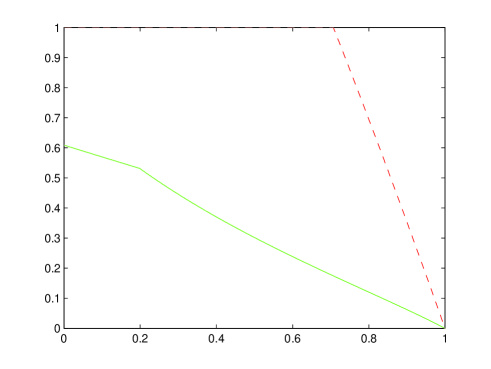
Figure 1. The function ${q}_{\rm succ}(\delta)$ is plotted in continuous line, while the function $q_{\rm fail}(\delta)$ is plotted in dashed line

2. Proofs

In this section, we give the proofs of Theorems 1.2, 1.3, 1.4 and 1.5.

2.1. Proof of Theorem 1.4

To prove Theorem 1.4, we need three technical lemmas.

Lemma 2.1.

Let $0<q\leq 1,0\leq c\leq 1$ and $a,b>0$. Then

(2.1) $$a+\sum_{k=1}^{m}t_{k}\leq\max\Big{\{}\max_{1\leq k\leq m}\frac{k+a}{(k+b)^{1/q}},\frac{a+c}{(b+c^{q})^{1/q}}\Big{\}}\Big{(}b+\sum_{k=1}^{m}t_{k}^{q}\Big{)}^{1/q}$$

holds for any $(t_{1},\ldots,t_{m})\in[0,1]^{m}$ with $t_{1}+\cdots+t_{m}\geq c$.

Proof.

Define

(2.2) $$F_{q,a,b,c}(m,n)=\sup_{\small\begin{array}[]{l}(t_{1},\ldots,t_{m})\in[0,1]^{m}\\ t_{1}+\cdots+t_{m}\geq c\end{array}}\frac{n+a+\sum_{k=1}^{m}t_{k}}{(n+b+\sum_{k=1}^{m}t_{k}^{q})^{1/q}}.$$

By the method of Lagrange multiplier, the function $(n+a+\sum_{k=1}^{m}t_{k})(n+b+\sum_{k=1}^{m}t_{k}^{q})^{-1/q}$ attains its maximum on the boundary or on those points $(t_{1},\ldots,t_{m})$ whose components are the same, i.e.,

$$F_{q,a,b,c}(m,n) = \max\Big{\{}F_{q,a,b,0}(m-1,n+1),F_{q,a,b,c}(m-1,n),$$

$$\qquad\qquad\sup_{c/m\leq t\leq 1}\frac{n+a+mt}{(n+b+mt^{q})^{1/q}}\Big{\}}.$$

As the function $(n+a+mt)(n+b+mt^{q})^{-1/q}$ has at most one critical point and the second derivative at that critical point (if it exists) is positive, we then have

(2.3) $$F_{q,a,b,c}(m,n) = \max\Big{\{}F_{q,a,b,0}(m-1,n+1),F_{q,a,b,c}(m-1,n),$$

$$\qquad\qquad\frac{n+m+a}{(n+m+b)^{1/q}},\frac{n+a+c}{(n+b+m^{1-q}c^{q})^{1/q}}\Big{\}}.$$

Applying (2.3) iteratively we obtain

(2.4) $$F_{q,a,b,c}(m,n) = \max\Big{\{}F_{q,a,b,0}(m-2,n+2),F_{q,a,b,0}(m-2,n+1),$$

$$\qquad F_{q,a,b,c}(m-2,n),\frac{n+1+a}{(n+1+b)^{1/q}},\frac{n+m-1+a}{(n+m-1+b)^{1/q}},$$

$$\qquad\frac{n+m+a}{(n+m+b)^{1/q}},\frac{n+a+c}{(n+b+(m-1)^{1-q}c^{q})^{1/q}}\Big{\}}$$

$$= \cdots$$

$$= \max\Big{\{}F_{q,a,b,0}(1,n+m-1),\cdots,F_{q,a,b,0}(1,n+1),$$

$$\qquad F_{q,a,b,c}(1,n),\frac{n+a+c}{(n+b+2^{1-q}c^{q})^{1/q}},$$

$$\qquad\frac{n+m+a}{(n+m+b)^{1/q}},\ldots,\frac{n+2+a}{(n+2+b)^{1/q}},\frac{n+1+a}{(n+1+b)^{1/q}}\Big{\}}$$

$$= \max\Big{\{}\max_{1\leq k\leq m}\frac{n+k+a}{(n+k+b)^{1/q}},\frac{n+a+c}{(n+b+c^{q})^{1/q}}\Big{\}}.$$

Then the conclusion (2.1) follows by letting $n=0$ in the above estimate. ∎

Lemma 2.2.

Let $0<q\leq 1$, $c_{1},c_{2}\in[0,1]$ and $a_{i},b_{i}>0$ for $i=1,2,3$. Then

(2.5) $$a_{1}+a_{2}x+a_{3}y+\sum_{k=1}^{m}t_{k}$$

$$\leq \max\Big{\{}\frac{a_{1}+a_{2}}{(b_{1}+b_{2})^{1/q}},\frac{a_{1}+a_{2}c_{1}}{(b_{1}+b_{2}c_{1}^{q})^{1/q}},\sup_{0\leq l\leq m}\frac{a_{1}+a_{2}+(a_{3}+l)c_{2}}{(b_{1}+b_{2}+(b_{3}+l)c_{2}^{q})^{1/q}},$$

$$\sup_{0\leq l\leq m}\frac{a_{1}+a_{2}c_{1}+(a_{3}+l)c_{2}}{(b_{1}+b_{2}c_{1}^{q}+(b_{3}+l)c_{2}^{q})^{1/q}}\Big{\}}\times\Big{(}b_{1}+b_{2}x^{q}+b_{3}y^{q}+\sum_{k=1}^{m}t_{k}^{q}\Big{)}^{1/q}$$

holds for all $0\leq t_{1},\ldots,t_{m}\leq y$, $c_{1}\leq x\leq 1$ and $0\leq y\leq c_{2}$.

Proof.

Note that the maximum values of the function $(a+bt)/(c+dt^{q})^{1/q}$ on any closed subinterval of $[0,\infty)$ are attained on its boundary. Then

$$\frac{a_{1}+a_{2}x+a_{3}y+\sum_{k=1}^{m}t_{k}}{(b_{1}+b_{2}x^{q}+b_{3}y^{q}+\sum_{k=1}^{m}t_{k}^{q})^{1/q}}$$

$$= \sup_{0\leq l\leq m}\frac{a_{1}+a_{2}x+(a_{3}+l)y}{(b_{1}+b_{2}x^{q}+(b_{3}+l)y^{q})^{1/q}}$$

$$= \max\Big{\{}\frac{a_{1}+a_{2}x}{(b_{1}+b_{2}x^{q})^{1/q}},\sup_{0\leq l\leq m}\frac{a_{1}+(a_{3}+l)c_{2}+a_{2}x}{(b_{1}+(b_{3}+l)c_{2}^{q}+b_{2}x^{q})^{1/q}}\Big{\}}$$

$$\leq \max\Big{\{}\frac{a_{1}+a_{2}}{(b_{1}+b_{2})^{1/q}},\frac{a_{1}+a_{2}c_{1}}{(b_{1}+b_{2}c_{1}^{q})^{1/q}},\sup_{0\leq l\leq m}\frac{a_{1}+a_{2}+(a_{3}+l)c_{2}}{(b_{1}+b_{2}+(b_{3}+l)c_{2}^{q})^{1/q}},$$

$$\sup_{0\leq l\leq m}\frac{a_{1}+a_{2}c_{1}+(a_{3}+l)c_{2}}{(b_{1}+b_{2}c_{1}^{q}+(b_{3}+l)c_{2}^{q})^{1/q}}\Big{\}},$$

and (2.5) follows. ∎

Lemma 2.3.

Let $0<q\leq 1$, $s\geq 1$ be a positive integer, and let $\{a_{j}\}_{j\geq 1}$ be a finite decreasing sequence of nonnegative numbers with

(2.6) $$\sum_{k\geq 1}\Big{(}\sum_{i=1}^{s}a_{ks+i}^{2}\Big{)}^{1/2}\geq\delta\Big{(}\sum_{i=1}^{s}|a_{i}|^{2}\Big{)}^{1/2}$$

for some $\delta\in(0,1)$. Then

(2.7) $$\sum_{k\geq 1}\Big{(}\sum_{i=1}^{s}a_{ks+i}^{2}\Big{)}^{1/2}\leq a(q,\delta)s^{1/2-1/q}\Big{(}\sum_{j\geq 1}a_{j}^{q}\Big{)}^{1/q},$$

where $a(q,\delta)$ is defined as in (1.12).

Proof.

Clearly the conclusion (2.7) holds when $a_{s+1}=0$ for in this case the left hand side of (2.7) is equal to 0. So we may assume that $a_{s+1}\neq 0$ from now on. Let $r_{0}$ be an arbitrarily number in $(0,1)$. To establish (2.7), we consider two cases.

Case I: $\sum_{k\geq 2}a_{ks+1}\geq r_{0}\delta a_{s+1}$.

In this case,

(2.8) $$\frac{\sum_{k\geq 1}\big{(}\sum_{i=1}^{s}a_{ks+i}^{2}\big{)}^{1/2}}{\big{(}\sum_{j\geq 1}a_{j}^{q}\big{)}^{1/q}}\leq\frac{s^{1/2}\sum_{k\geq 1}a_{ks+1}}{s^{1/q}\big{(}\sum_{k\geq 1}a_{ks+1}^{q}\big{)}^{1/q}}$$

$$= s^{1/2-1/q}\frac{1+\sum_{k\geq 2}a_{ks+1}/a_{s+1}}{\big{(}1+\sum_{k\geq 2}(a_{ks+1}/a_{s+1})^{q}\big{)}^{1/q}}$$

$$\leq s^{1/2-1/q}\max\Big{\{}\frac{1+r_{0}\delta}{(1+r_{0}^{q}\delta^{q})^{1/q}},\max_{k\geq 1}\frac{k+1}{(k+1)^{1/q}}\Big{\}}$$

$$= s^{1/2-1/q}(1+r_{0}\delta)(1+r_{0}^{q}\delta^{q})^{-1/q},$$

where the first inequality holds because $\{a_{j}\}_{j\geq 1}$ is a decreasing sequence of nonnegative numbers, the second inequality follows from Lemma 2.1, and the last equality is true as $(1+t)(1+t^{q})^{-1/q}$ is a decreasing function on $(0,1]$.

Case II: $\sum_{k\geq 2}a_{ks+1}<r_{0}\delta a_{s+1}$.

Let $s_{0}$ be the smallest integer in $[1,s]$ satisfying $a_{s+s_{0}+1}/a_{s+1}\leq(s_{0}/s)^{1/2}$. The existence and uniqueness of such an integer $s_{0}$ follow from the decreasing property of the sequence $\{a_{s+s_{0}+1}/a_{s+1}\}_{s_{0}=1}^{s}$, the increasing property of the sequence $\{(s_{0}/s)^{1/2}\}_{s_{0}=1}^{s}$, and $a_{s+s_{0}+1}/a_{s+1}\leq(s_{0}/s)^{1/2}$ when $s_{0}=s$. Then from the decreasing property of the sequence $\{a_{j}\}_{j\geq 1}$ and the definition of the integer $s_{0}$ it follows that

(2.9) $$\frac{a_{s+s_{0}}}{a_{s+1}}\geq\big{(}\frac{s_{0}-1}{s}\big{)}^{1/2}$$

and

$$\sqrt{2}s_{0}^{1/2}a_{s+1} \geq \big{(}s_{0}a_{s+1}^{2}+(s-s_{0})\frac{s_{0}}{s}a_{s+1}^{2}\big{)}^{1/2}\geq\Big{(}\sum_{i=1}^{s}a_{s+i}^{2}\Big{)}^{1/2}$$

$$\geq \delta\Big{(}\sum_{i=1}^{s}a_{i}^{2}\Big{)}^{1/2}-\sum_{k\geq 2}\Big{(}\sum_{i=1}^{s}a_{ks+i}^{2}\Big{)}^{1/2}$$

$$\geq \delta s^{1/2}a_{s+1}-s^{1/2}\sum_{k\geq 2}a_{ks+1}\geq(1-r_{0})\delta s^{1/2}a_{s+1},$$

which implies that

(2.10) $$s_{0}\geq\frac{(1-r_{0})^{2}\delta^{2}}{2}s.$$

Applying the decreasing property of the sequence $\{a_{j}\}$ and using the inequality $(\theta a^{2}+(1-\theta)b^{2})^{1/2}\leq\theta^{1/2}a+(1-\theta^{1/2})b$ where $a\geq b\geq 0$ and $\theta\in[0,1]$, we obtain

(2.11) $$s^{-1/2}\sum_{k\geq 1}\Big{(}\sum_{i=1}^{s}a_{ks+i}^{2}\Big{)}^{1/2}$$

$$\leq s^{-1/2}\big{(}(s_{0}-1)a_{s+1}^{2}+a_{s+s_{0}}^{2}+(s-s_{0})a_{s+s_{0}+1}^{2}\big{)}^{1/2}$$

$$+s^{-1/2}\sum_{k\geq 2}\big{(}s_{0}a_{ks+1}^{2}+(s-s_{0})a_{ks+s_{0}+1}^{2}\big{)}^{1/2}$$

$$\leq \sqrt{\frac{s_{0}}{s}}\Big{(}\frac{s_{0}-1}{s_{0}}a_{s+1}^{2}+\frac{1}{s_{0}}a_{s+s_{0}}^{2}\Big{)}^{1/2}+\Big{(}1-\sqrt{\frac{s_{0}}{s}}\Big{)}a_{s+s_{0}+1}$$

$$+\sum_{k\geq 2}\Big{(}\sqrt{\frac{s_{0}}{s}}a_{ks+1}+\Big{(}1-\sqrt{\frac{s_{0}}{s}}\Big{)}a_{ks+s_{0}+1}\Big{)}$$

$$\leq \sqrt{\frac{s_{0}-1}{s}}a_{s+1}+\frac{\sqrt{s_{0}}-\sqrt{s_{0}-1}}{\sqrt{s}}a_{s+s_{0}}+\sum_{k\geq 1}a_{ks+s_{0}+1},$$

and

(2.12) $$\sum_{j\geq 1}a_{j}^{q} \geq (s+1)a_{s+1}^{q}+(s_{0}-1)a_{s+s_{0}}^{q}$$

$$\quad+a_{s+s_{0}+1}^{q}+s\sum_{k\geq 2}a_{ks+s_{0}+1}^{q}.$$

Combining (2.11) and (2.12), recalling (2.9) and the definition of the integer $s_{0}$, and applying Lemma 2.2 with $c_{1}=\sqrt{(s_{0}-1)/s}$ and $c_{2}=\sqrt{s_{0}/s}$, we get

(2.13) $$s^{1/q-1/2}\frac{\sum_{k\geq 1}\big{(}\sum_{i=1}^{s}a_{ks+i}^{2}\big{)}^{1/2}}{\big{(}\sum_{j\geq 1}a_{j}^{q}\big{)}^{1/q}}$$

$$\leq \frac{\sqrt{\frac{s_{0}-1}{s}}a_{s+1}+\frac{\sqrt{s_{0}}-\sqrt{s_{0}-1}}{\sqrt{s}}a_{s+s_{0}}+a_{s+s_{0}+1}+\sum_{k\geq 2}a_{ks+s_{0}+1}}{\big{(}(1+1/s)a_{s+1}^{q}+(s_{0}-1)a_{s+s_{0}}^{q}/s+a_{s+s_{0}+1}^{q}/s+\sum_{k\geq 2}a_{ks+s_{0}+1}^{q}\big{)}^{1/q}}$$

$$\leq \max\Big{\{}\frac{\sqrt{\frac{s_{0}}{s}}}{\big{(}1+s_{0}/s\big{)}^{1/q}},\frac{\sqrt{\frac{s_{0}-1}{s}}\Big{(}1+\frac{\sqrt{s_{0}}-\sqrt{s_{0}-1}}{\sqrt{s}}\Big{)}}{\big{(}1+1/s+((s_{0}-1)/s)^{1+q/2}\big{)}^{1/q}},$$

$$\sup_{l\geq 0}\frac{(l+2)\sqrt{\frac{s_{0}}{s}}}{\big{(}1+s_{0}/s+(l+1/s)\sqrt{\frac{s_{0}}{s}}\big{)}^{1/q}},$$

$$\sup_{l\geq 0}\frac{(l+1)\sqrt{\frac{s_{0}}{s}}+\sqrt{\frac{s_{0}-1}{s}}\Big{(}1+\frac{\sqrt{s_{0}}-\sqrt{s_{0}-1}}{\sqrt{s}}\Big{)}}{\big{(}\big{(}(l+1/s)\sqrt{\frac{s_{0}}{s}}+1+1/s\big{)}+((s_{0}-1)/s)^{1+q/2}\big{)}^{1/q}}\Big{\}}.$$

Therefore

(2.14) $$\frac{\sum_{k\geq 1}\big{(}\sum_{i=1}^{s}a_{ks+i}^{2}\big{)}^{1/2}}{\big{(}\sum_{j\geq 1}a_{j}^{q}\big{)}^{1/q}}$$

$$\leq s^{1/2-1/q}\max\Big{\{}\frac{\sqrt{{s_{0}}/{s}}}{\big{(}1+s_{0}/s\big{)}^{1/q}},\frac{\sqrt{{s_{0}}/{s}}}{\big{(}1+2^{-q/2}(s_{0}/s)^{1+q/2}\big{)}^{1/q}},$$

$$\sup_{l\geq 0}\frac{(l+2)\sqrt{{s_{0}}/{s}}}{\big{(}1+s_{0}/s+l\sqrt{{s_{0}}/{s}}\big{)}^{1/q}},\sup_{l\geq 0}\frac{(l+2)\sqrt{{s_{0}}/{s}}}{\big{(}1+l\sqrt{{s_{0}}/{s}}+2^{-q/2}(s_{0}/s)^{1+q/2}\big{)}^{1/q}}\Big{\}}$$

$$\leq s^{1/2-1/q}\max\Big{\{}\frac{2\sqrt{{s_{0}}/{s}}}{\big{(}1+2^{-q/2}(s_{0}/s)^{1+q/2}\big{)}^{1/q}},\ \sup_{l\geq 1}\frac{(l+2)\sqrt{{s_{0}}/{s}}}{(1+l\sqrt{{s_{0}}/{s}}\big{)}^{1/q}}\Big{\}}$$

$$\leq s^{1/2-1/q}\max\Big{\{}\sup_{\sqrt{2}(1-r_{0})\delta/2\leq y\leq 1}\frac{2y}{\big{(}1+2^{-q/2}y^{2+q}\big{)}^{1/q}},$$

$$\quad\sup_{\sqrt{2}(1-r_{0})\delta/2\leq y\leq 1}\frac{3y}{\big{(}1+y\big{)}^{1/q}},\ \sup_{1\leq y}\frac{2y}{\big{(}1+y\big{)}^{1/q}}\Big{\}},$$

where the third inequality is valid by (2.10) and the first inequality follows from the following two inequalities:

(2.15) $$\sqrt{\frac{t-1}{s}}\Big{(}1+\frac{\sqrt{t}-\sqrt{t-1}}{\sqrt{s}}\Big{)}\leq\sqrt{\frac{t}{s}}$$

and

(2.16) $$\frac{1}{s}+\Big{(}\frac{t-1}{s}\Big{)}^{1+q/2}\geq\Big{(}\frac{1}{s}\Big{)}^{1+q/2}+\Big{(}\frac{t-1}{s}\Big{)}^{1+q/2}\geq 2^{-q/2}\Big{(}\frac{t}{s}\Big{)}^{1+q/2},\quad 1\leq t\leq s.$$

The conclusion (2.7) follows from (2.8) and (2.14). ∎

Now we give the proof of Theorem 1.4.

Proof of Theorem 1.4.

Let ${\bf h}$ satisfy

(2.17) $${\bf Ah}={\bf 0}$$

and let $S_{0}$ be a subset of $\{1,\ldots,n\}$ with cardinality $\#S_{0}$ less than or equal to $s$. We partition $S_{0}^{c}\subset\{1,\ldots,n\}$ as $S_{0}^{c}=S_{1}\cup\cdots\cup S_{l}$, where $S_{1}$ is the set of indices of the $s$ largest components, in absolute value, of ${\bf h}$ in $S_{0}^{c}$, $S_{2}$ is the set of indices of the next $s$ largest components, in absolute value, of ${\bf h}$ in $(S_{0}\cup S_{1})^{c}$, and so on. Applying the parallelogram identity, we obtain from the restricted isometry property (1.5) that

(2.18) $$|\langle{\bf Au},{\bf Av}\rangle|\leq\delta_{2s}({\bf A})\|{\bf u}\|_{2}\|{\bf v}\|_{2}$$

for all $s$-sparse vectors ${\bf u},{\bf v}\in\Sigma_{s}$ whose supports have empty intersection [7]. Combining (2.17) and (2.18) and using the restricted isometry property (1.5) yield

(2.19) $$(1-\delta_{2s}({\bf A}))\Big{(}\|{\bf h}_{S_{0}}\|_{2}^{2}+\|{\bf h}_{S_{1}}\|_{2}^{2})$$

$$\leq \langle{\bf A}({\bf h}_{S_{0}}+{\bf h}_{S_{1}}),{\bf A}({\bf h}_{S_{0}}+{\bf h}_{S_{1}})\rangle$$

$$\leq \big{\langle}{\bf A}\big{(}\sum_{i\geq 2}{\bf h}_{S_{i}}\big{)},{\bf A}\big{(}\sum_{j\geq 2}{\bf h}_{S_{j}}\big{)}\big{\rangle}$$

$$\leq \sum_{i,j\geq 2}\delta_{2s}({\bf A})\|{\bf h}_{S_{i}}\|_{2}\|{\bf h}_{S_{j}}\|_{2}+\sum_{j\geq 2}\|{\bf h}_{S_{j}}\|_{2}^{2}$$

$$= \delta_{2s}({\bf A})\Big{(}\sum_{j\geq 2}\|{\bf h}_{S_{j}}\|_{2}\Big{)}^{2}+\sum_{j\geq 2}\|{\bf h}_{S_{j}}\|_{2}^{2}$$

$$\leq (1+\delta_{2s}({\bf A}))\Big{(}\sum_{j\geq 2}\|{\bf h}_{S_{j}}\|_{2}\Big{)}^{2},$$

which implies that

(2.20) $$\sum_{j\geq 2}\|{\bf h}_{S_{j}}\|_{2}\geq\Big{(}\frac{1-\delta_{2s}({\bf A})}{1+\delta_{2s}({\bf A})}\Big{)}^{1/2}\|{\bf h}_{S_{1}}\|_{2}.$$

Applying Lemma 2.3 with $\delta_{1}=\big{(}\frac{1-\delta_{2s}({\bf A})}{1+\delta_{2s}({\bf A})}\big{)}^{1/2}$ gives

(2.21) $$\sum_{j\geq 2}\|{\bf h}_{S_{j}}\|_{2}\leq a(q,\delta_{1})s^{1/2-1/q}\|{\bf h}_{S_{0}^{c}}\|_{q}.$$

Then substituting the above estimate for $\sum_{j\geq 2}\|{\bf h}_{S_{j}}\|_{2}$ into the right hand side of the inequality (2.19) and recalling that ${\bf h}_{S_{0}}$ is an $s$-sparse vector lead to

(2.22) $$\|{\bf h}_{S_{0}}\|_{q}\leq s^{1/q-1/2}\|{\bf h}_{S_{0}}\|_{2}\leq s^{1/q-1/2}(\delta_{1})^{-1}\sum_{j\geq 2}\|{\bf h}_{S_{j}}\|_{2}\leq\frac{a(q,\delta_{1})}{\delta_{1}}\|{\bf h}_{S_{0}^{c}}\|_{q},$$

the desired null space property. ∎

2.2. Proof of Theorem 1.5

We follow the argument in [4, 5]. Set ${\bf h}={\bf x}^{*}-{\bf x}$, and denote by $S_{0}$ the support of the vector ${\bf x}_{s}\in\Sigma_{s}$, by $S_{0}^{c}$ the complement of the set $S_{0}$ in $\{1,\ldots,n\}$. Then

(2.23) $$\|{\bf Ah}\|_{2}=\|{\bf A}{\bf x}^{*}-{\bf A}{\bf x}\|_{2}\leq\|{\bf A}{\bf x}^{*}-{\bf y}\|_{2}+\|{\bf z}\|_{2}\leq 2\epsilon$$

and

(2.24) $$\|{\bf h}_{S_{0}^{c}}\|_{q}^{q}\leq\|{\bf h}_{S_{0}}\|_{q}^{q}+2\|{\bf x}-{\bf x}_{s}\|_{q}^{q},$$

since

$$\|{\bf x}_{s}\|_{q}^{q}+\|{\bf x}_{{}_{S_{0}^{c}}}\|_{q}^{q} = \|{\bf x}\|_{q}^{q}\geq\|{\bf x}^{*}\|_{q}^{q}=\|{\bf x}_{s}+{\bf h}_{{}_{S_{0}}}\|_{q}^{q}+\|{\bf x}_{{}_{S_{0}^{c}}}+{\bf h}_{{}_{S_{0}^{c}}}\|_{q}^{q}$$

$$\geq \|{\bf x}_{s}\|_{q}^{q}-\|{\bf h}_{{}_{S_{0}}}\|_{q}^{q}+\|{\bf h}_{S_{0}^{c}}\|_{q}^{q}-\|{\bf x}_{{}_{S_{0}^{c}}}\|_{q}^{q}.$$

Similar to the argument used in the proof of Theorem 1.4, we partition $S_{0}^{c}\subset\{1,\ldots,n\}$ as $S_{0}^{c}=S_{1}\cup\cdots\cup S_{l}$, where $S_{1}$ is the set of indices of the $s$ largest absolute-value component of ${\bf h}$ in $S_{0}^{c}$, $S_{2}$ is the set of indices of the next $s$ largest absolute-value components of ${\bf h}$ on $S_{0}^{c}$, and so on. Then it follows from (1.5), (2.19) and (2.23) that

(2.25) $$(1-\delta_{2s}({\bf A}))\big{(}\|{\bf h}_{S_{0}}\|_{2}^{2}+\|{\bf h}_{S_{1}}\|_{2}^{2}\big{)}$$

$$\leq \langle{\bf A}({\bf h}_{S_{0}}+{\bf h}_{S_{1}}),{\bf A}({\bf h}_{S_{0}}+{\bf h}_{S_{1}})\rangle$$

$$\leq \big{\langle}{\bf A}{\bf h}-{\bf A}\big{(}\sum_{i\geq 2}{\bf h}_{S_{i}}\big{)},{\bf A}{\bf h}-{\bf A}\big{(}\sum_{j\geq 2}{\bf h}_{S_{j}}\big{)}\big{\rangle}$$

$$\leq \big{(}2\epsilon+\sqrt{1+\delta_{2s}({\bf A})}\sum_{j\geq 2}\|{\bf h}_{S_{j}}\|_{2}\big{)}^{2}.$$

By the continuity of the function $a(q,\delta)$ about $\delta\in(0,1)$ and the assumption (1.14), there exists a positive number $r$ such that

(2.26) $$a(q,\delta_{1}/(1+r))<\delta_{1}/(1+r).$$

If $\sum_{j\geq 2}\|{\bf h}_{S_{j}}\|_{2}\leq 2\epsilon/(r\sqrt{1+\delta_{2s}({\bf A})})$, then it follows from (2.24), (2.25) and the fact that ${\bf h}_{S_{0}}\in\Sigma_{s}$ that

(2.27) $$\|{\bf x}^{*}-{\bf x}\|_{2} = \|{\bf h}\|_{2}\leq\big{(}\|{\bf h}_{S_{0}}\|_{2}^{2}+\|{\bf h}_{S_{1}}\|_{2}^{2})^{1/2}+\sum_{j\geq 2}\|{\bf h}_{S_{j}}\|_{2}$$

$$\leq 2\Big{(}\frac{(1+r)}{r\sqrt{1-\delta_{2s}({\bf A})}}+\frac{1}{r\sqrt{1+\delta_{2s}({\bf A})}}\Big{)}\epsilon,$$

and

(2.28) $$\|{\bf x}^{*}-{\bf x}\|_{q}^{q} \leq \|{\bf h}_{S_{0}}\|_{q}^{q}+\|{\bf h}_{S_{0}^{c}}\|_{q}^{q}\leq 2\|{\bf h}_{S_{0}}\|_{q}^{q}+2\|{\bf x}-{\bf x}_{s}\|_{q}^{q}$$

$$\leq 2s^{1-q/2}\|{\bf h}_{S_{0}}\|_{2}^{q}+2\|{\bf x}-{\bf x}_{s}\|_{q}^{q}$$

$$\leq 2^{1+q}\frac{(1+r)^{q}}{r^{q}(1-\delta_{2s}({\bf A}))^{q/2}}s^{1-q/2}\epsilon^{q}+2\|{\bf x}-{\bf x}_{s}\|_{q}^{q}.$$

If $\sum_{j\geq 2}\|{\bf h}_{S_{j}}\|_{2}\geq 2\epsilon/(r\sqrt{1+\delta_{2s}({\bf A})})$, then

(2.29) $$\delta_{1}\big{(}\|{\bf h}_{S_{0}}\|_{2}^{2}+\|{\bf h}_{S_{1}}\|_{2}^{2}\big{)}^{1/2}\leq(1+r)\sum_{j\geq 2}\|{\bf h}_{S_{j}}\|_{2}$$

by (2.25), where we set $\delta_{1}=\sqrt{(1-\delta_{2s}({\bf A}))/(1+\delta_{2s}({\bf A}))}$. Using (2.29) and applying Lemma 2.3 with $\delta=\delta_{1}/(1+r)$ give

(2.30) $$\sum_{j\geq 2}\|{\bf h}_{S_{j}}\|_{2}\leq a(q,\delta_{1}/(1+r))s^{1/2-1/q}\|{\bf h}_{S_{0}^{c}}\|_{q}.$$

Noting the fact that ${\bf h}_{S_{0}}\in\Sigma_{s}$ and then applying (2.24), (2.29) and (2.30) yield

$$\|{\bf h}_{S_{0}}\|_{q}^{q} \leq s^{1-q/2}\|{\bf h}_{S_{0}}\|_{2}^{q}\leq\Big{(}\frac{a(q,\delta_{1}/(1+r))}{\delta_{1}/(1+r)}\Big{)}^{q}\|{\bf h}_{S_{0}^{c}}\|_{q}^{q}$$

$$\leq \Big{(}\frac{a(q,\delta_{1}/(1+r))}{\delta_{1}/(1+r)}\Big{)}^{q}\|{\bf h}_{S_{0}}\|_{q}^{q}+2\Big{(}\frac{a(q,\delta_{1}/(1+r))}{\delta_{1}/(1+r)}\Big{)}^{q}\|{\bf x}-{\bf x}_{s}\|_{q}^{q}.$$

This, together with (2.26), leads to the following crucial estimate:

(2.31) $$\|{\bf h}_{S_{0}}\|_{q}^{q}\leq\frac{2(a(q,\delta_{1}/(1+r)))^{q}}{(\delta_{1}/(1+r))^{q}-(a(q,\delta_{1}/(1+r)))^{q}}\|{\bf x}-{\bf x}_{s}\|_{q}^{q}.$$

Combining (2.24), (2.29), (2.30) and (2.31), we obtain

(2.32) $$\|{\bf x}^{*}-{\bf x}\|_{2} \leq \big{(}\|{\bf h}_{S_{0}}\|_{2}^{2}+\|{\bf h}_{S_{1}}\|_{2}^{2})^{1/2}+\sum_{j\geq 2}\|{\bf h}_{S_{j}}\|_{2}$$

$$\leq \frac{2^{1/q}(1+r+\delta_{1})\big{(}a(q,\delta_{1}/(1+r))\big{)}^{2}}{\delta_{1}\big{(}(\delta_{1}/(1+r))^{q}-(a(q,\delta_{1}/(1+r)))^{q}\big{)}^{1/q}}s^{1/2-1/q}\|{\bf x}-{\bf x}_{s}\|_{q},$$

and

(2.33) $$\|{\bf x}^{*}-{\bf x}\|_{q}^{q} \leq 2\|{\bf h}_{S_{0}}\|_{q}^{q}+2\|{\bf x}-{\bf x}_{s}\|_{q}^{q}$$

$$\leq \frac{2(\delta_{1}/(1+r))^{q}+2(a(q,\delta_{1}/(1+r)))^{q}}{(\delta_{1}/(1+r))^{q}-(a(q,\delta_{1}/(1+r)))^{q}}\|{\bf x}-{\bf x}_{s}\|_{q}^{q}.$$

The desired error estimates (1.16) and (1.17) follow from (2.27), (2.28), (2.32) and (2.33).

2.3. Proof of Theorem 1.2

The conclusion in Theorem 1.2 follows from Corollary 1.6 and the observation that

(2.34) $$\lim_{q\to 0+}a(q,\delta)=0$$

for any $\delta\in(0,1)$.

2.4. Proof of Theorem 1.3

Let

(2.35) $$\tilde{q}_{\max}(\delta_{1})=\sup\{q\in(0,1]|\ a(q,\delta_{1})<\delta_{1}\}.$$

Take sufficiently small $\epsilon>0$. Note that

(2.40) $$\sup_{\sqrt{2}(1-r_{0})\delta_{1}/2\leq y\leq 1}\frac{2y}{\big{(}1+2^{-q/2}y^{2+q}\big{)}^{1/q}}$$

$$= \left\{\begin{array}[]{l}\frac{\sqrt{2}(1-r_{0})\delta_{1}}{\big{(}1+2^{-1-q}((1-r_{0})\delta_{1})^{2+q}\big{)}^{1/q}}\\ \qquad{\rm if}\ q<2^{-q}(1-r_{0})^{2+q}\delta_{1}^{2+q},\\ q^{1/(2+q)}\big{(}1+\frac{q}{2}\big{)}^{-1/q}2^{(1+3q/2)/(2+q)}\\ \qquad{\rm if}\ 1\geq q\geq 2^{-q}(1-r_{0})^{2+q}\delta_{1}^{2+q}.\end{array}\right.$$

Then for any small $q>(e/2+\epsilon)\delta_{1}^{2}$ and sufficiently small $\delta_{1}>0$, we have that $q\geq 2^{-q}(1-r_{0})^{2+q}\delta_{1}^{2+q}$ for all $r_{0}\in(0,1)$. Then applying (1.12) and (2.40) yields

$$a(q,\delta_{1}) \geq \inf_{0<r_{0}<1}\sup_{\sqrt{2}(1-r_{0})\delta_{1}/2\leq y\leq 1}\frac{2y}{\big{(}1+2^{-q/2}y^{2+q}\big{)}^{1/q}}$$

$$= q^{1/(2+q)}\big{(}1+\frac{q}{2}\big{)}^{-1/q}2^{(1+3q/2)/(2+q)}$$

$$\geq (1+\epsilon/e)^{1/2}\delta_{1},$$

where the last inequality holds since

(2.41) $$\lim_{q\to 0}q^{-q/(4+2q)}\big{(}1+\frac{q}{2}\big{)}^{-1/q}2^{(1+3q/2)/(2+q)}=(2/e)^{1/2}.$$

Therefore

(2.42) $$\limsup_{\delta_{1}\to 0}\frac{\tilde{q}_{\max}(\delta_{1})}{\delta_{1}^{2}}\leq\limsup_{\delta_{1}\to 0}\frac{(e/2+\epsilon)\delta_{1}^{2}}{\delta_{1}^{2}}\leq\frac{e}{2}+\epsilon$$

for any sufficiently small $\epsilon>0$.

Take $r_{0}=1-\sqrt{2}/4$ and sufficiently small $\epsilon>0$. Then for $q\leq(e/2-\epsilon)\delta_{1}^{2}$ and sufficiently small $\delta_{1}>0$,

(2.43) $$\left\{\begin{array}[]{l}(1+r_{0}\delta_{1})(1+r_{0}^{q}\delta_{1}^{q})^{-1/q}\leq 2(3/2)^{-1/q}\leq(1-\epsilon/e)^{1/2}\delta_{1},\\ \sup_{y\geq 1}y(1+y)^{-1/q}\leq\sup_{y\geq 1}(1+y)^{1-1/q}\leq 2^{1-1/q}\leq(1-\epsilon/e)^{1/2}\delta_{1}/2,\\ \sup_{y\geq\sqrt{2}(1-r_{0})\delta_{1}/2}\frac{y}{(1+y)^{1/q}}=\frac{\sqrt{2}(1-r_{0})\delta_{1}/2}{(1+\sqrt{2}(1-r_{0})\delta/2)^{1/q}}\leq(1-\epsilon/e)^{1/2}\delta_{1}/3,\end{array}\right.$$

and

(2.44) $$\sup_{\sqrt{2}(1-r_{0})\delta_{1}/2\leq y\leq 1}\frac{2y}{\big{(}1+2^{-q/2}y^{2+q}\big{)}^{1/q}}\leq(1-\epsilon/e)^{1/2}\delta_{1}$$

by (1.12), (2.40) and (2.41). Therefore

(2.45) $$\liminf_{\delta_{1}\to 0}\frac{\tilde{q}_{\max}(\delta_{1})}{\delta_{1}^{2}}\geq\limsup_{\delta_{1}\to 0}\frac{(e/2-\epsilon)\delta_{1}^{2}}{\delta_{1}^{2}}\geq\frac{e}{2}-\epsilon$$

by (2.43) and (2.44). Combining (2.42) and (2.45) and recalling that $\epsilon>0$ is a sufficiently small number chosen arbitrarily, we have

(2.46) $$\lim_{\delta_{1}\to 0}\frac{\tilde{q}_{\max}(\delta_{1})}{\delta_{1}^{2}}=\frac{e}{2}.$$

By Corollary 1.6, we have

(2.47) $$q_{\max}(\delta;m,n,s)\geq\tilde{q}_{\max}(\sqrt{(1-\delta)/(1+\delta)}).$$

This together with (2.46) implies that

(2.48) $$\liminf_{\delta\to 1-}\frac{q_{\max}(\delta;m,n,s)}{1-\delta}\geq\lim_{\delta\to 1-}\frac{\tilde{q}_{\max}(\sqrt{(1-\delta)/(1+\delta)})}{(1-\delta)/(1+\delta)}\times\frac{1}{1+\delta}=\frac{e}{4},$$

and hence completes the proof.

Acknowledgement  Part of this work is done when the author is visiting Vanderbilt University and Ecole Polytechnique Federale de Lausanne on his sabbatical leave. The author would like to thank Professors Akram Aldroubi, Douglas Hardin, Michael Unser and Martin Vetterli for the hospitality and fruitful discussion, and Professor R. Chartrand for his comments on the early version of this manuscript.

References

- [1] T. Blu, P.L. Dragotti, M. Vetterli, P. Marziliano and L. Coulot, Sparse sampling of signal innovations, IEEE Signal Processing Magazine, 25(2008), 31–40.
- [2] S. Boyd and L. Vandenberghe, Convex Optimization, Cambridge University Press, Cambridge, 2004.
- [3] T. T. Cai, L. Wang and G. Xu, Shifting inequality and recovery of sparse signals, IEEE Trans. Signal Process., 58(2010), 1300–1308.
- [4] E. J. Candes, The restricted isometry property and its implications for compressed sensing, C. R. Acad. Sci. Paris, Ser. I, 346(2008), 589–592.
- [5] E. J. Candes, J. Romberg and T. Tao, Stable signal recovery from incomplete and inaccurate measurements, Comm. Pure Appl. Math., 59(2006), 1207–1223.
- [6] E. J. Candes, J. Romberg and T. Tao, Robust uncertainty principles: exact signal reconstruction from highly incomplete frequency information, IEEE Trans. Inform. Theory, 52(2006), 489–509.
- [7] E. J. Candes and T. Tao, Decoding by linear programming, IEEE Trans. Inform. Theory, 51(2005), 4203–4215.
- [8] E. J. Candes and W. B. Wakin, Enhancing sparsity by reweighted minimization, J. Fourier Anal. Appl., 14(2008), 877–905.
- [9] R. Chartrand, Exact reconstruction of sparse signals via nonconvex minimization, IEEE Signal Proc. Letter, 14(2007), 707–710.
- [10] R. Chartrand and V. Staneva, Restricted isometry properties and nonconvex compressive sensing, Inverse Problems, 24(2008), 035020 (14 pp).
- [11] X. Chen, F. Xu and Y. Ye, Lower bound theory of nonzero entries in solution of - minimization, Preprint 2009.
- [12] A. Cohen, W. Dahmen and R. DeVore, Compressive sensing and best -term approximation, J. Amer. Math. Soc., 22(2009), 211–231.
- [13] M. E. Davies and R. Gribonval, Restricted isometry constants where sparse recovery can fail for , IEEE Trans. Inform. Theorey, 55(2009), 2203–2214.
- [14] I. Dauchebies, R. DeVore, M. Fornasier, and C. S. Gunturk, Iteratively re-weighted least squares minimization for sparse recovery, Commun. Pure Appl. Math., 63(2010), 1–38.
- [15] D. Donoho and M. Elad, Optimally sparse representation in general (nonorthogonal) dictionaries via norm minimization, Proc. Nat. Acad. Sci. USA, 100(2003), 2197–2002.
- [16] S. Foucart, A note on guaranteed sparse recovery via -minimization, Appl. Comput. Harmonic Anal., DOI 10.1016/j.acha.2009.10.004
- [17] S. Foucart and M.-J. Lai, Sparsest solutions of underdetermined linear system via -minimization for , Appl. Comput. Harmonic Anal., 26(2009), 395–407.
- [18] G. Gribonval and M. Nielsen, Highly sparse representations from dictionaries are unique and independent of the sparseness measure, Appl. Comput. Harmonic Anal., 22(2007), 335–355.
- [19] X. Jiang and Y. Ye, A note on complexity of minimization, Preprint 2009.
- [20] B. K. Natarajan, Sparse approximate solutions to linear systems, SIAM J. Comput., 24(1995), 227–234.
- [21] B. D. Rao and K. Kreutz-Delgado, An affine scaling methodology for best basis selection, IEEE Trans. Signal Process., 47(1999), 187–200.
- [22] R. Saab, R. Chartrand, O. Yilmaz, Stable sparse approximations via nonconvex optimization, In IEEE International Conference on Acoustics, Speech and Signal Processing (ICASSP), 2008, 3885–3888.
- [23] R. Saab and O. Yilmaz, Sparse recovery by non-convex optimization – instance optimality, Appl. Comput. Harmonic Anal., doi:10.1016/j.acha.2009.08.002