Distance growth of quantum states due to initial system–environment correlations

Abstract

Intriguing features of the distance between two arbitrary states of an open quantum system are identified that are induced by initial system-environment correlations. As an example, we analyze a qubit dephasingly coupled to a bosonic environment. Within tailored parameter regimes, initial correlations are shown to substantially increase a distance between two qubit states evolving to long-time limit states according to exact non-Markovian dynamics. It exemplifies the breakdown of the distance contractivity of the reduced dynamics.

Introduction. –There are various states of physical systems changing and evolving in time. Thermodynamic states or quantum states are well known examples. One can pose natural questions: How ”similar” is a given nonequilibrium state to the equilibrium one? How ”similar” is an entangled quantum state to the unentangled one? Is there a natural quantifier to measure the separation between states? The answer is not unique and depends on a character of a problem which we analyze. In the simplest way, we could say that two states are close to each other if averaged values of observables in these states are close to each other. For quantum systems, there is a natural distance induced by a norm which in turn is induced by the scalar product of vectors in Hilbert space of a given quantum system. One of the central issues of quantum engineering is to prepare a quantum system in a state having desired features. Doing this one is faced with many difficulties: unavoidable decoherence, imperfect implementation of quantum operations and many other sources of unpredictable mess. The statistical similarity of quantum states can be related to certain measures of a distance between them gil . One of the most popular quantifiers for the distiguishability of the probability distributions arising from the measurements conducted on quantum states (or shortly ’distinguishability of states’) is the trace distance nielsen . The trace distance of any two states (density matrices) $\rho_{1}$ and $\rho_{2}$ is defined as nielsen

$$D[\rho_{1},\rho_{2}]=||\rho_{1}-\rho_{2}||,$$ (1)

where for any operator $A$ its norm is defined by the relation $||A||=(1/2)\,\mbox{Tr}\sqrt{A^{\dagger}A}$. Any positive and trace-preserving map $\cal E$ defined on the whole space of trace class operators on the Hilbert space is contractive, i.e.

$$D[{\cal E}(\rho_{1}),{\cal E}(\rho_{2})]\leq D[\rho_{1},\rho_{2}].$$ (2)

In particular, when ${\cal E}={\cal E}_{t}$ is a completely positive quantum dynamical semigroup such that $\rho(t)={\cal E}_{t}\rho(0)$, then

$$D[\rho_{1}(t),\rho_{2}(t)]\leq D[\rho_{1}(s),\rho_{2}(s)]\quad\mbox{for}\quad t>s,$$ (3)

i.e. the distance cannot increase in time. It means that the distinguishability of any states can not increase above an initial value. Motivated by findings recently reported in Ref. breu3 , we study an open quantum system which is initially correlated with its environment pech . We consider a dephasing model defaz ; devoret of decoherence of a qubit interacting with a bosonic environment. If the qubit and its environment is initially prepared in an uncorrelated state, the reduced dynamics is completely positive and hence contractive. In the presence of initial correlations one is left with positive (but non completely positive) dynamics zycz ; ban and the contractivity may fail breu3 . The model of dephasing allows to find an exact reduced dynamics and reveals highly non-trivial properties of distinguishability with respect to the trace distance. We explicitly show that under tailored regimes the contractivity fails for some initially entangled states. The trace distance of different states grows above its initial value even in the long time limit. In consequence, the distinguishability of the long-time limit states can increase above its initial value.

Model. –The system we study is a qubit $Q$, formed by an arbitrary two-level system coupled to its environment $B$. We consider the case when the process of energy dissipation is negligible and only pure decoherence is a mechanism for decoherence of the qubit. It leads to an irreversible process of information loss. We model such a system by the Hamiltonian ($\hbar=1$)

$$H=H_{Q}\otimes{\mathbb{I}}_{B}+{\mathbb{I}}_{Q}\otimes H_{B}+S^{z}\otimes H_{I},$$ (4)

$$H_{Q}=\varepsilon S^{z},\quad H_{B}=\int_{0}^{\infty}d\omega\,h(\omega)a^{\dagger}(\omega)a(\omega),$$ (5)

$$H_{I}=\int_{0}^{\infty}d\omega\left[g^{*}(\omega)a(\omega)+g(\omega)a^{\dagger}(\omega)\right],$$ (6)

where $S^{z}$ is the z-component of the spin operator and is represented by the diagonal matrix $S^{z}=diag[1,-1]$ of elements $1$ and $-1$. The parameter $\varepsilon$ is the qubit energy splitting, ${\mathbb{I}}_{Q}$ and ${\mathbb{I}}_{B}$ are identity operators (matrices) in corresponding Hilbert spaces of the qubit $Q$ and the environment $B$, respectively. The operators $a^{\dagger}(\omega)$ and $a(\omega)$ are the bosonic creation and annihilation operators, respectively. The real-valued spectrum function $h(\omega)$ characterizes the environment. The coupling is described by the function $g(\omega)$ and the function $g^{*}(\omega)$ is the complex conjugate to $g(\omega)$. The Hamiltonian (4) can be rewritten in the block–diagonal structure fidel ,

$$H=diag[H_{+},H_{-}],\quad H_{\pm}=H_{B}\pm H_{I}\pm\varepsilon{\mathbb{I}}_{B}.$$ (7)

We consider a correlated initial state of the qubit–environment system in the form similar to that in Ref. kossak , namely,

$$|\Psi(0)\rangle=b_{+}|1\rangle\otimes|\Omega_{0}\rangle+b_{-}|-1\rangle\otimes|\Omega_{\lambda}\rangle.$$ (8)

The states $|1\rangle$ and $|-1\rangle$ denote the excited and ground states of the qubit, respectively, the non-zero complex numbers $b_{+}$ and $b_{-}$ are such that $|b_{+}|^{2}+|b_{-}|^{2}=1$. The states $|\Omega_{0}\rangle$ and $|\Omega_{\lambda}\rangle$ are environment states. As an example, let us assume that $|\Omega_{0}\rangle$ is an environment ground state and

$$|\Omega_{\lambda}\rangle=C_{\lambda}^{-1}\,\left[(1-\lambda)|\Omega_{0}\rangle+\lambda|\Omega_{f}\rangle\right]$$ (9)

is a linear combination of a ground state $|\Omega_{0}\rangle$ and the coherent state $|\Omega_{f}\rangle=D(f)|\Omega_{0}\rangle$, where the displacement operator $D(f)$ reads brat

$$D(f)=\exp\left\{\int_{0}^{\infty}d\omega\left[f(\omega)a^{\dagger}(\omega)-f^{*}(\omega)a(\omega)\right]\right\}$$ (10)

for an arbitrary square–integrable function $f$. The constant $C_{\lambda}$ normalizes the state $|\Omega_{\lambda}\rangle$ and reads

$$C_{\lambda}^{2}=(1-\lambda)^{2}+\lambda^{2}+2\lambda(1-\lambda)Re\langle\Omega_{0}|\Omega_{f}\rangle,$$ (11)

where ${Re}$ is a real part of the scalar product $\langle\Omega_{0}|\Omega_{f}\rangle$ of two states in the environment Hilbert space. The parameter $\lambda\in[0,1]$ controls the initial entanglement of the qubit and environment. For $\lambda=0$ the qubit and environment are initially uncorrelated while for $\lambda=1$ the entanglement is, for a given class of initial states, maximal. The states with $\lambda=1$ are not maximally entangled in the usual sense as the coherent states, forming an overcomplete set of states, are not mutually orthogonal. The state of the total system at time $t>0$ has the form

$$|\Psi(t)\rangle=b_{+}|1\rangle\otimes|\psi_{+}(t)\rangle+b_{-}|-1\rangle\otimes|\psi_{-}(t)\rangle,$$ (12)

where $|\psi_{+}(t)\rangle=\exp(-iH_{+}t)|\Omega_{0}\rangle$ and $|\psi_{-}(t)\rangle=\exp(-iH_{-}t)|\Omega_{\lambda}\rangle$. The density matrix $\rho_{\lambda}(t)$ of the qubit is obtained from the relation

$$\rho_{\lambda}(t)=\mbox{Tr}_{B}\left\{|\Psi(t)\rangle\langle\Psi(t)|\right\}$$ (13)

and $\mbox{Tr}_{B}$ denotes the partial tracing over the environment. Its explicit form reads

$$\rho_{\lambda}(t)=\left(\begin{array}[]{cc}|b_{+}|^{2}&b_{+}b_{-}^{*}A_{\lambda}(t)\\ b_{+}^{*}b_{-}A_{\lambda}^{*}(t)&|b_{-}|^{2}\end{array}\right),$$ (16)

$$A_{\lambda}(t)=C_{\lambda}^{-1}\,e^{-2i\varepsilon t}e^{-r(t)}\,\left[1-\lambda+\lambda e^{-2i\Phi(t)}e^{s(t)}\right],$$ (17)

where fidel

$$r(t)=4\int_{0}^{\infty}d\omega g_{h}^{2}(\omega)\left[1-\cos(\omega t)\right],\quad\quad\quad\quad\quad$$

$$s(t)=2\int_{0}^{\infty}d\omega g_{h}(\omega)f(\omega)\left[1-\cos(\omega t)\right]-\frac{1}{2}\int_{0}^{\infty}d\omega f^{2}(\omega),\quad$$

where $g_{h}(\omega)=g(\omega)/h(\omega)$ and

$$\Phi(t)=\int_{0}^{\infty}d\omega g_{h}(\omega)f(\omega)\sin(\omega t).$$ (18)

For the sake of simplicity, we have assumed that the functions $g(\omega)$ and $f(\omega)$ are real. The modeling of the qubit coupling to the environment is performed in terms of the spectral density function

$$g_{h}^{2}(\omega)=\alpha\,\omega^{\mu-1}\exp(-\omega/\omega_{c}),$$ (19)

where $\alpha>0$ is the qubit-environment coupling constant, $\mu>-1$ is the ”ohmicity” parameter (the case $\mu=0$ corresponds to the ohmic and $\mu>0$ to super-ohmic environments, respectively) and $\omega_{c}$ is a cut-off frequency. The coherent state $|\Omega_{f}\rangle$ is determined by the function

$$f^{2}(\omega) = \gamma\,\omega^{\nu-1}\exp(-\omega/\omega_{c}).$$ (20)

This choice is arbitrary but convenient as it allows for finding an explicte analytic formulas for

$$r(t)=4\mathcal{L}(\alpha,\mu,t)],\quad\quad\quad$$

$$s(t)=2\mathcal{L}(\sqrt{\alpha\gamma},(\mu+\nu)/2,t)-\gamma\Gamma(\nu)\omega_{c}^{\nu},$$

$$\mathcal{L}(\alpha,\mu,t)=\lambda\Gamma(\nu)\omega_{c}^{\mu}\left\{1-\frac{\cos\left[\mu\arctan(\omega_{c}t)\right]}{(1+\omega_{c}^{2}t^{2})^{\mu/2}}\right\},$$

$$\Phi(t)=\sqrt{\alpha\gamma}\;\Gamma(\kappa)\omega_{c}^{\kappa}\;\frac{\sin\left[\kappa\arctan(\omega_{c}t)\right]}{(1+\omega_{c}^{2}t^{2})^{\kappa/2}},\quad$$ (21)

where $\Gamma(\nu)$ is the Euler gamma function and the parameter $\kappa=(\mu+\nu)/2$.

Distance of states. –Let us examine the distinguishability between two various, initially correlated ($\lambda\neq 0$) states. The corresponding trace distance reads

$$D^{2}[\rho_{\lambda_{1}}(t),\rho_{\lambda_{2}}(t)]=\left(|b_{+}^{(1)}|^{2}-|b_{+}^{(2)}|^{2}\right)^{2}$$

$$+|b_{+}^{(1)}b_{-}^{(1)*}A_{\lambda_{1}}(t)-b_{+}^{(2)}b_{-}^{(2)*}A_{\lambda_{2}}(t)|^{2}.$$ (22)

As the initial state (8) of the qubit–environment composite system is generically entangled, the non–local operations are involved in its preparation. Such a procedure would essentially require highly sophisticated quantum engineering. Naively speaking one can recognize the following steps: (i) the first, when one prepares the state $|\Omega_{\lambda}\rangle$ given by Eq. (9), next ”tensorize” it with the ground state of the qubit $|-1\rangle$; (ii) the second step, when one superpose, with the weights $b_{\pm}$, the result of the first step with the excited qubit $|1\rangle$ state tensorized with the vacuum $|\Omega_{0}\rangle$. Both steps demand using precise technics and their details are essentially beyond the scope of this paper. A different preparations of initial states (8) can be provided both via changing details of the first step and the second step of the procedure. In other words, one can change the parameters $b_{\pm}$ in (8) or manipulate on the state $|\Omega_{\lambda}\rangle$ (by changing $\lambda$). When two different states are determined by two different sets of numbers $b_{\pm}^{(k)}\;(k=1,2)$ in the superposition (8) with the same state $|\Omega_{\lambda}\rangle$ then $A_{\lambda_{1}}(t)=A_{\lambda_{2}}(t)$ and Eq. (Distance growth of quantum states due to initial system–environment correlations) takes the form

$$D^{2}[\rho_{\lambda_{1}}(t),\rho_{\lambda_{2}}(t)]=\left(|b_{+}^{(1)}|^{2}-|b_{+}^{(2)}|^{2}\right)^{2}$$

$$+|b_{+}^{(1)}b_{-}^{(1)*}-b_{+}^{(2)}b_{-}^{(2)*}|^{2}\;|A_{\lambda_{1}}(t)|^{2}.$$ (23)

The function $|A_{\lambda_{1}}(t)|$ is a decaying function of time and the distance (Distance growth of quantum states due to initial system–environment correlations) also decays as time grows. In consequence the distinguishability between two initially correlated states always becomes lowered. It is clear that no matter what $b_{\pm}^{(k)}$ are, the reduced dynamics results in contraction of the distance between the states. So, the only chance to observe the growth of the distinguishability of qubit reduced states is to modify the parameters of environment encoded in $|\Omega_{\lambda}\rangle$ in Eq.(9).

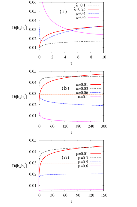
Figure 1: Time evolution of the trace distance $D[\rho_{\lambda}(t),\rho_{0}(t)]$ between the initially correlated and non-correlated states for selected values of parameters. Dimensionless time is in unit of $\omega_{c}$. The remaining parameters are: $\varepsilon=1,(a)\mu=0.01$, $\nu=0.05$, $\alpha=0.01,\gamma=0.05$; (b) $\mu=0.01$, $\nu=0.05$ , $\gamma=0.05$. $\lambda=0.25$; (c) $\nu=0.05$ , $\gamma=0.05$. $\lambda=0.25$, $\alpha=0.01$. The horizontal lines in (b) and (c) indicate the initial distance.

Let us consider this case assuming that $b_{\pm}^{(k)}=b_{\pm}$ are fixed and the same for $k=1,2$, and two different states are determined by two different sets of numbers $\lambda_{1}$ and $\lambda_{2}$. In such a case the distance reads

$$|b_{+}b_{-}^{*}|^{-1}\;D[\rho_{\lambda_{1}}(t),\rho_{\lambda_{2}}(t)]=|A_{\lambda_{1}}(t)-A_{\lambda_{2}}(t)|$$

$$=e^{-r(t)}\left\{a^{2}+b^{2}e^{2s(t)}+2abe^{s(t)}\cos[2\Phi(t)]\right\}^{1/2},$$ (24)

where

$$a=\frac{1-\lambda_{1}}{C_{\lambda_{1}}}-\frac{1-\lambda_{2}}{C_{\lambda_{2}}},\quad b=\frac{\lambda_{1}}{C_{\lambda_{1}}}-\frac{\lambda_{2}}{C_{\lambda_{2}}}.$$ (25)

In Fig. 1(a), we show time evolution of the trace distance $D[\rho_{\lambda}(t),\rho_{0}(t)]$ between the initially correlated and non-correlated states for four selected degrees of correlation determined by the value of the correlation parameter $\lambda$. At time $t=0$, the distance $D=0.004,0.03,0.08,0.19$ for $\lambda=0.1,0.25,0.4,0.6$, respectively. In the long time limit, the distance between states takes the values $D=0.03,0.08,0.12,0.15$, respectively. In the first three cases, the distance between long-time limit states is greater than the initial distance and the distinguishability of final states is better than initial states. There is some optimal correlation $\lambda$ for which the distinguishability of final states is the best. However, if the initial correlation is strong enough, the distance for long time is smaller than at the initial time. It is important observation that there exists a critical value $\lambda_{c}$ (depending on other parameters) such that for $\lambda>\lambda_{c}$ the stationary states are less distinguishable than initial states. In some regimes (as e.g. the case $\lambda=0.25,0.4$ in Fig. 1(a)), at early stage of evolution, the distance decreases reaching a minimum and next it increases and saturates for long time. In Fig. 1(b) and Fig. 1(c) we show how the distance can depend on environment characteristics: the coupling constant $\alpha$ and the ”super-ohmicity” $\mu>0$. It follows that strong coupling of the qubit to environment diminishes the distinguishability of initial states. Similarly, if the environment is more super-ohmic, the distinguishability of states is weaker.

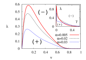
Figure 2: In the region limited by the curves and the horizontal axes (denoted by $+$), $\lim_{t\to\infty}D[\rho_{\lambda_{1}}(t),\rho_{0}(t)]>D[\rho_{\lambda_{1}}(0),\rho_{0}(0)]$. Outside this region (denoted by $-$), the distance between two states at time $t=0$ is greater than between the long-time limit states (the contractive region). The parameters are: $\varepsilon=1$, $\gamma=0.05,\mu=0.01$; Inset: $\mu=0.01,\nu=0.05$.

In Fig. 2, the influence of parameters characterizing initial environment state is depicted. Both regions, where the ”distinguishability gain” (i. e. the distance in the long time limit is greater than for the initial time) is reached, are limited and located in the corner of the corresponding parameter planes. It means that not all but specific environments can induce the ”distinguishability gain”.

Finally, we consider the case when both $\lambda_{1}$ and $\lambda_{2}$ are non-zero, see Fig. 3. At time $t=0$, the distance is $D=0.015,0.014,0.0071,0.026$ for $\lambda=0,0.05,0.3,0.4$, respectively. In the long time limit, the distance takes the values $D=0.039,0.031,0.0072,0.020$, respectively. In the first three cases, the final distance is greater than the initial distance and the distinguishability of final states is better than initial states. The region of the $(\lambda_{1},\lambda_{2})$-plane, where this effect occurs is bounded by $\lambda_{1}$ and $\lambda_{2}$ axes and a decreasing function $\lambda_{2}$ vs $\lambda_{1}$. From the presented example we detect that if $\lambda_{2}$ exceeds some fixed value of $\lambda_{1}$, this effect is distinctly absent and the distance in the long time limit can never be greater than for $t=0$.

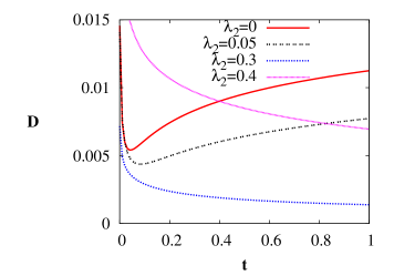
Figure 3: Time evolution of the trace distance $D[\rho_{\lambda_{1}}(t),\rho_{\lambda_{2}}(t)]$ for fixed $\lambda_{1}=0.25$ and several values of $\lambda_{2}$. Time is scaled as in Fig. 1. The parameters $\mu=0.01$, $\nu=0.05$ $\alpha=0.01$, $\gamma=0.25$ and $b_{+}=b_{-}=1/\sqrt{2}$.

Summary. –Recent investigations have often shown that dynamics of quantum systems can exhibit various counter–intuitive and non–trivial features which can be inferred from detailed analysis of highly sophisticated theoretical models. It is of great importance to verify the predictions in a carefully prepared experiments. An effective design of such experiments would require guidelines provided by theoretical studies of realistic physical models. Our work reported in this paper, as a step in this direction, could be placed somewhere in between: we consider a fairly simple model of decoherence under very specific conditions but present results which are exact. Despite its simplicity the model is realistic enough to be experimentally accessible devoret . According to common wisdom the decoherence resulting from the ”openness” of quantum systems causes blurring of the information encoded in quantum states: as it has recently been shown breu3 in the context of distinguishability of quantum states, it is not always the case. In this paper we provide an explicit realization of the recent suggestion on the distinguishability growth due to initial qubit–environment entanglement. The distinguishability growth occurs not only at the short time scales but is shown to be a feature of long-time limit states. This feature seems to be favorable for the potential experimental verification of the predictions presented in breu3 especially when the desired short–time growth would occur in ultra–short time scales. We have shown that the induced distinguishability growth is not generic for the considered model and we identified the parameter regimes where the effect is the most apparent.

The work supported by the ESF Program ”Exploring the Physics of Small Devices”.

References

- (1) A. Gilchrist et al., Phys. Rev. A 71, 062310 (2005).
- (2) M. A. Nielsen and L. I. Chuang, Quantum Computation and Quantum Information (Cambridge University Press, Cambridge, U.K., 2000).
- (3) E.–M. Laine et al., arxiv:1004.2184v1 (2010).
- (4) P. Pechukas, Phys. Rev. Lett. 73, 1060 (1994); P. Stelmachovic and V. Buzek, Phys. Rev. A 64, 062106 (2001); N. Boulant et al., J. Chem. Phys. 121, 2955 (2004); F. Jordan et al., Phys. Rev. A 70, 052110 (2004).
- (5) D. I. Schuster et al., Nature 445 515 (2007).
- (6) J. Łuczka, Physica A 167, 919 (1990).
- (7) M. Ban, Phys. Rev. A 80, 064103 (2009).
- (8) H. A. Carteret et al., Phys. Rev. A 77, 042113 (2008).
- (9) J. Dajka and J. Łuczka, Phys. Rev. A 77, 062303 (2008); J. Dajka et al., Phys. Rev. A 79, 012104 (2009).
- (10) P. Anielo et al., Open Sys. & Inf. Dyn. (accepted), arXiv:0912.4123 (2009).
- (11) O. Brattelli and D. W. Robinson, Operator Algebras and Quantum Statistical Mechanics 2 (Springer, Berlin, 1997).