Quenched exit estimates and ballisticity conditions for higher-dimensional random walk in random environment

Abstract

Consider a random walk in an i.i.d. uniformly elliptic environment in dimensions larger than one. In 2002, Sznitman introduced for each $\gamma\in(0,1)$ the ballisticity condition $(T)_{\gamma}$ and the condition $(T^{\prime})$ defined as the fulfillment of $(T)_{\gamma}$ for each $\gamma\in(0,1)$. Sznitman proved that $(T^{\prime})$ implies a ballistic law of large numbers. Furthermore, he showed that for all $\gamma\in(0.5,1)$, $(T)_{\gamma}$ is equivalent to $(T^{\prime})$. Recently, Berger has proved that in dimensions larger than three, for each $\gamma\in(0,1)$, condition $(T)_{\gamma}$ implies a ballistic law of large numbers. On the other hand, Drewitz and Ramírez have shown that in dimensions $d\geq 2$ there is a constant $\gamma_{d}\in(0.366,0.388)$ such that for each $\gamma\in(\gamma_{d},1)$, condition $(T)_{\gamma}$ is equivalent to $(T^{\prime})$. Here, for dimensions larger than three, we extend the previous range of equivalence to all $\gamma\in(0,1)$. For the proof, the so-called effective criterion of Sznitman is established employing a sharp estimate for the probability of atypical quenched exit distributions of the walk leaving certain boxes. In this context, we also obtain an affirmative answer to a conjecture raised by Sznitman in 2004 concerning these probabilities. A key ingredient for our estimates is the multiscale method developed recently by Berger.

and

t1Supported in part by the International Research Training Group “Stochastic Models of Complex Processes.” t2Supported in part by the Berlin Mathematical School. t3Supported in part by Fondo Nacional de Desarrollo Científico y Tecnológico Grant 1100298.

1 Introduction and statement of the main results

We continue our investigation of the interrelations between the ballisticity conditions $(T)_{\gamma}$ and $(T^{\prime})$ introduced by Sznitman in Sz-02 for random walk in random environment (RWRE). In dimensions larger than or equal to four, the results we establish in this paper amount to a considerable improvement of what has been obtained in our work DrRa-09b. To prove the corresponding results, we take advantage of techniques recently developed by Berger in Be-09. We derive sharp estimates on the probability of certain quenched exit distributions of the RWRE and thereby provide an affirmative answer to a slightly stronger version of a conjecture announced by Sznitman in Sz-04.

We start by giving an introduction to the model, thereby fixing the notation we employ. Denote by $\mathcal{M}_{d}$ the space of probability measures on the set $\{e\in\mathbb{Z}^{d}\dvtx\|e\|_{1}=1\}$ of canonical unit vectors and set $\Omega:=(\mathcal{M}_{d})^{\mathbb{Z}^{d}}$. For each environment $\omega=(\omega(x,\cdot))_{x\in\mathbb{Z}^{d}}\in\Omega$, we consider the Markov chain $(X_{n})_{n\in\mathbb{N}}$ with transition probabilities from $x$ to $x+e$ given by $\omega(x,e)$ for $\|e\|_{1}=1$, and $0$ otherwise. We denote by $P_{x,\omega}$ the law of this Markov chain conditioned on $\{X_{0}=x\}$. Furthermore, let $\mathbb{P}$ be a probability measure on $\Omega$ such that the coordinates $(\omega(x,\cdot))_{x\in\mathbb{Z}^{d}}$ of the environment $\omega$ are i.i.d. under $\mathbb{P}$. Then $\mathbb{P}$ is called elliptic if $\mathbb{P}(\min_{\|e\|_{1}=1}\omega(0,e)>0)=1$ while it is called uniformly elliptic if there is a constant $\kappa>0$ such that $\mathbb{P}(\min_{\|e\|_{1}=1}\omega(0,e)\geq\kappa)=1.$ We call $P_{x,\omega}$ the quenched law of the RWRE starting from $x$, and correspondingly we define the averaged (or annealed) law of the RWRE by $P_{x}:=\int_{\Omega}P_{x,\omega}\mathbb{P}(d\omega)$.

Given a direction $l\in\mathbb{S}^{d}$, we say that the RWRE is transient in the direction $l$ if

$$P_{0}\Bigl{(}\lim_{n\to\infty}X_{n}\cdot l=\infty\Bigr{)}=1.$$

Furthermore, we say that the RWRE is ballistic in the direction $l$ if $P_{0}$-a.s.

$$\liminf_{n\to\infty}\frac{X_{n}\cdot l}{n}>0.$$

It is well known that in dimension one there exists uniformly elliptic RWRE in i.i.d. environments which is transient but not ballistic to the right. It was also recently established that in dimensions larger than one there exists elliptic RWRE in i.i.d. environments which is transient but not ballistic in a given direction see Sabot and Tournier in SaTo-09. Nevertheless, the following fundamental conjecture remains open.

Conjecture 1.1.

In dimensions larger than one, every uniformly elliptic RWRE in an i.i.d. environment which is transient in a given direction is necessarily ballistic in the same direction.

Some partial progress has been made toward the resolution of this conjecture by studying transient RWRE satisfying some additional assumptions introduced in Sz-02, usually called ballisticity conditions. For each $l\in\mathbb{S}^{d-1}$ and $L>0$, let us define

$$T_{L}^{l}:=\inf\{n\geq 0\dvtx X_{n}\cdot l>L\}.$$

Definition 1.2.

Let $\gamma\in(0,1)$ and $l\in\mathbb{S}^{d-1}$. We say that condition $(T)_{\gamma}$ is satisfied with respect to $l$ [written $(T)_{\gamma}|l$ or $(T)_{\gamma}$] if for each $l^{\prime}$ in a neighborhood of $l$ and each $b>0$ one has that

$$\limsup_{L\to\infty}L^{-\gamma}\log P_{0}(T_{L}^{l^{\prime}}>T_{bL}^{-l^{\prime}})<0.$$

We say that condition $(T^{\prime})$ is satisfied with respect to $l$ [written $(T^{\prime})|l$ or $(T^{\prime})$], if for each $\gamma\in(0,1)$, condition $(T)_{\gamma}|l$ is fulfilled.

It is known that in dimensions $d\geq 2$, condition $(T^{\prime})$ implies the existence of a deterministic $v\in\mathbb{R}^{d}\setminus\{0\}$ such that $P_{0}$-a.s. $\lim_{n\to\infty}\frac{X_{n}}{n}=v$, as well as a central limit theorem for the RWRE so that under the annealed law $P_{0}$,

$$B^{n}_{\cdot}:=\frac{X_{{\lfloor\cdot n\rfloor}}-{\lfloor\cdot n\rfloor}v}{n}$$

converges in distribution to a Brownian motion in the Skorokhod space $D([0,\infty)$, $\mathbb{R}^{d})$ as $n\to\infty$; see, for instance, Theorem 4.1 in Sz-04 for further details. Recently, in Be-09 the author has shown that in dimensions larger than three, the above law of large numbers and central limit theorem remain valid if condition $(T)_{\gamma}$ is satisfied for some $\gamma\in(0,1)$. In addition, in Sz-04 the author has proven that if $\mathbb{P}$ is uniformly elliptic, then in dimensions $d\geq 2$, for each $\gamma\in(0.5,1)$ and each $l\in\mathbb{S}^{d-1}$, condition $(T)_{\gamma}|l$ is equivalent to $(T^{\prime})|l$. In DrRa-09b, the authors pushed down this equivalence to each $\gamma\in(\gamma_{d},1)$, where $\gamma_{d}\in(0.366,0.388)$ is decreasing with the dimension. The first main result of the present paper is a considerable improvement of these previous results for dimensions larger than three.

Theorem 1.3

Let $d\geq 4$ and $\mathbb{P}$ be uniformly elliptic. Then for all $\gamma\in(0,1)$ and $l\in\mathbb{S}^{d-1}$, condition $(T)_{\gamma}|l$ is equivalent to $(T^{\prime})|l$.

The proof of Theorem 1.3 takes advantage of the effective criterion and is therefore closely related to upper bounds for quenched probabilities of atypical exit behavior of the RWRE. To state the corresponding result, denote for any subset $B\subset\mathbb{Z}^{d}$ its boundary by

$$\partial B:=\{x\in\mathbb{Z}^{d}\setminus B\dvtx\exists y\in B\mbox{ such that }\|x-y\|_{1}=1\}$$

and define the slab

$$U_{\beta,l,L}:=\{x\in\mathbb{Z}^{d}\dvtx-L^{\beta}\leq x\cdot l\leq L\}.$$

Furthermore, for the rest of this paper we let

$$T_{B}:=\inf\{n\in\mathbb{N}_{0}\dvtx X_{n}\in B\}$$

denote the first hitting time. For $x\in\mathbb{Z}^{d}$ set $T_{x}:=T_{\{x\}}$. In terms of this notation, in Sz-04 the author conjectured the following (cf. Figure 1).

Conjecture 1.4.

Let $d\geq 2$, $\mathbb{P}$ be uniformly elliptic and assume $(T^{\prime})|l$ to hold for some $l\in\mathbb{S}^{d-1}$. Fix $c>0$ and $\beta\in(0,1)$. Then for all $\alpha\in(0,\beta d)$,

$$\limsup_{L\to\infty}L^{-\alpha}\log\mathbb{P}\bigl{(}P_{0,\omega}(X_{T_{\partial U_{\beta,l,L}}}\cdot l>0)\leq e^{-cL^{\beta}}\bigr{)}<0.$$

Theorem 4.4 of Sz-04 states that the above conjecture holds true for all positive $\alpha$ with

$$\alpha<d\biggl{(}(2\beta-1)\vee\frac{2\beta}{d+1}\biggr{)}.$$

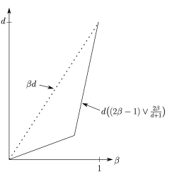
Figure 1: Sketch of the known and conjectured bounds for $\alpha$.

The second main result of the present paper gives an affirmative answer to a seemingly stronger statement than the one of Conjecture 1.4. For $l\in\mathbb{S}^{d-1}$, denote by

$$\pi_{l}\dvtx\mathbb{R}^{d}\ni x\quad\mapsto\quad(x\cdot l)l\in\mathbb{R}^{d}$$

the orthogonal projection on the space $\{\lambda l\dvtx\lambda\in\mathbb{R}\}$ as well as by

$$\pi_{l^{\bot}}\dvtx\mathbb{R}^{d}\ni x\quad\mapsto\quad x-\pi_{l}(x)\in\mathbb{R}^{d}$$

the orthogonal projection on the orthogonal complement $\{\lambda l\dvtx\lambda\in\mathbb{R}\}^{\bot}$. Using this notation, for $K>0$ we define the box

$$B_{L,l,K}:=\{x\in\mathbb{Z}^{d}\dvtx 0\leq x\cdot l\leq L,\|\pi_{l^{\bot}}(x)\|_{\infty}\leq KL\}$$

as well as its right boundary part

$$\partial_{+}B_{L,l,K}:=\{x\in\partial B_{L,l,K}\dvtx x\cdot l>L\},$$ (1)

see Figure 2.

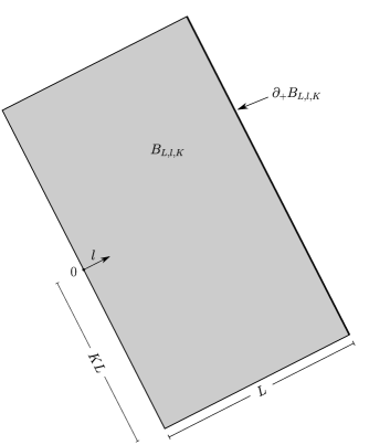
Figure 2: The set $B_{L,l,K}$ and its boundary part $\partial_{+}B_{L,l,K}$.

We can now state the desired result.

Theorem 1.5

Let $d\geq 4$, $\mathbb{P}$ be uniformly elliptic and assume $(T)_{\gamma}|l$ to hold for some $\gamma\in(0,1)$, $l\in\mathbb{S}^{d-1}$. Fix $c>0$ and $\beta\in(0,1)$. Then there exists a constant $K>0$ such that for all $\alpha\in(0,\beta d)$,

$$\limsup_{L\to\infty}L^{-\alpha}\log\mathbb{P}\bigl{(}P_{0,\omega}(T_{\partial B_{L,l,K}}=T_{\partial_{+}B_{L,l,K}})\leq e^{-cL^{\beta}}\bigr{)}<0.$$

Remark 1.6.

[(a)]

The result we prove is slightly stronger than the conjecture announced in Sz-04 since we can dispose of the extent of the slab in direction $-l$ as well as restrict the extent in directions orthogonal to $l$. Scrutinizing the proof it will be clear that one can improve this result replacing the box $B_{L,l,K}$ by a parabola-shaped set which grows in the directions transversal to $\hat{v}$ at least like $L^{\alpha}$ for some $\alpha>1/2$.

Note that this theorem is optimal in the sense that its conclusion will not hold in general for $\alpha>\beta d$. In fact, for plain nestling RWRE, this can be shown by the use of so-called naïve traps (see Sz-04, page 244).

In both, Theorem 1.3 as well as Theorem 1.5, the restriction to dimensions larger than three is caused by the following: for a very large set of environments we need that the trajectories of two independent $d$-dimensional random walks in this environment intersect only very rarely; see equations (LABEL:eq:JNProb) and (LABEL:eq:JHittingProbBd).

The proof of Theorem 1.5 exploits heavily a recent multiscale technique introduced in Be-09 to study the slowdown upper bound for RWRE. To explain this in more detail, note that from that source one also infers that every RWRE in a uniformly elliptic i.i.d. environment which satisfies condition $(T)_{\gamma}$ for some $\gamma\in(0,1)$, has an asymptotic speed $v\neq 0$. The main result of Be-09 states that for every RWRE in a uniformly elliptic i.i.d. environment satisfying condition $(T)_{\gamma}$, some $\gamma\in(0,1)$, the following holds: for each $a\neq v$ in the convex hull of $0$ and $v$ as well as $\epsilon>0$ small enough, and any $\alpha<d$ the inequality

$$P_{0}\biggl{(}\biggl{\|}\frac{X_{n}}{n}-a\biggr{\|}_{\infty}<\epsilon\biggr{)}\leq\exp\{-(\log n)^{\alpha}\}$$

holds for all $n$ large enough. To prove the above result, Berger develops a multiscale technique which describes the behavior of the walk at the scale of the so called naïve traps, which at time $n$ are of radius of order $\log n$. Here, we rely on such a multiscale technique to make explicit the role of the regions of the same scale as the naïve traps to prove Theorem 1.5.

In Section 2, we show how certain exit estimates from boxes imply Theorem 1.5 and how in turn such a result implies Theorem 1.3. In Section 3, we start with giving a heuristic explanation of a modified version of Berger’s multiscale technique and of how to deduce the aforementioned exit estimates. We then set up our framework of notation and auxiliary results before making precise the previous heuristics by giving the corresponding proofs. In the Appendix we establish several specific results concerning local limit theorem type results and estimates involving intersections of random walks.

2 Proofs of the main results

The proofs of Theorems 1.3 and 1.5 are based on a multiscale argument and a semi-local limit theorem developed in Be-09 for RWRE in dimensions larger than or equal to four.

It is well known that if for some $\gamma\in(0,1)$ and $l\in\mathbb{S}^{d-1}$, condition $(T)_{\gamma}|l$ is fulfilled, then $P_{0}$-a.s. the limit

$$\hat{v}:=\lim_{n\to\infty}\frac{X_{n}}{\|X_{n}\|_{2}}\in\mathbb{S}^{d-1}$$

exists and is constant (cf., e.g., Theorem 1 in Simenhaus Si-07); it is called the asymptotic direction.

Define for a vector $e_{j}$ of the canonical basis of $\mathbb{Z}^{d}$ and $l\in\mathbb{S}^{d-1}$ such that $l\cdot e_{j}\neq 0$ the projection $\tilde{\pi}^{j}_{l}$ via

$$\tilde{\pi}^{j}_{l}\dvtx\mathbb{R}^{d}\ni x\quad\mapsto\quad\frac{x\cdot e_{j}}{l\cdot e_{j}}l\in\mathbb{R}^{d}$$

on the space $\{\lambda l\dvtx\lambda\in\mathbb{R}\}$ and by $\tilde{\pi}^{j}_{l^{\bot}}$ the projection

$$\tilde{\pi}^{j}_{l^{\bot}}\dvtx\mathbb{R}^{d}\ni x\quad\mapsto\quad x-\frac{x\cdot e_{j}}{l\cdot e_{j}}l\in\mathbb{R}^{d}$$

on the space $\{\lambda e_{j}\dvtx\lambda\in\mathbb{R}\}^{\bot}$. In the case $j=1$, we will abbreviate this notation by $\tilde{\pi}_{l}$ and $\tilde{\pi}_{l^{\bot}}$. For $j\in\{1,\ldots,d\}$, $\delta>0$ and $L>0$, define the set

$$C_{L}:=\{x\in\mathbb{Z}^{d}\dvtx 0\leq x\cdot e_{j}\leq L^{1+\delta},\|\tilde{\pi}^{j}_{\hat{v}^{\bot}}(x)\|_{\infty}\leq L^{3\delta}+x\cdot e_{j}L^{-2\delta}\};$$

cf. Figure 3. In analogy to (1), we introduce the right boundary parts

$$\partial_{+}C_{L}:=\{x\in\partial C_{L}\dvtx x\cdot e_{j}>L^{1+\delta}\}$$

and $\partial_{+}(x+C_{L}):=x+\partial_{+}C_{L}$ for $x\in\mathbb{Z}^{d}$.

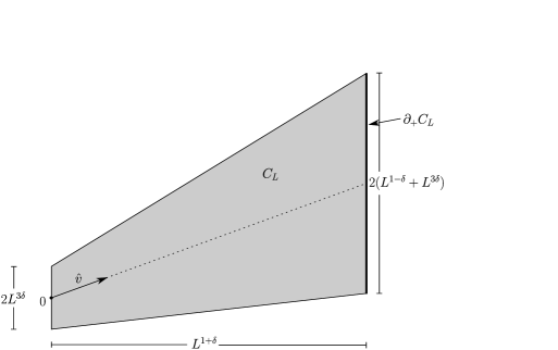
Figure 3: The set $C_{L}$ and its boundary part $\partial_{+}C_{L}$.

The proof of the following proposition will be deferred to Section 3.

Proposition 2.1

Let $d\geq 4$, $\mathbb{P}$ be uniformly elliptic and assume $(T)_{\gamma}|l$ to hold for some $\gamma\in(0,1)$, $l\in\mathbb{S}^{d-1}$. Without loss of generality, let $e_{j}$ be a vector of the canonical basis such that $\hat{v}\cdot e_{j}>0$ and fix $\beta\in(0,1)$ as well as $\alpha\in(0,\beta d)$.

Then for all $\delta>0$ small enough there exists a sequence of events $(\Xi_{L})_{L\in\mathbb{N}}$ such that for all $L$ large enough we have

$$\inf_{\omega\in\Xi_{L}}P_{0,\omega}(T_{\partial C_{L}}=T_{\partial_{+}C_{L}})\geq e^{-L^{\beta-\delta}}$$

and

$$\mathbb{P}(\Xi_{L}^{c})\leq e^{-L^{\alpha}}.$$

For the sake of notational simplicity and without loss of generality, we assume $j=1$ from now on.

2.1 Proof of Theorem 1.5

We will show that Theorem 1.5 is a consequence of Proposition 2.1. For this purpose, let the assumptions of Theorem 1.5 be fulfilled. In particular, let $(T)_{\gamma}|l$ be fulfilled (which implies $l\cdot\hat{v}>0$; cf. Theorem 1.1 of Sz-02) and fix $c>0$, $\beta\in(0,1)$ as well as $\alpha\in(0,\beta d)$. Let $\delta>0$ small enough such that the implication of Proposition 2.1 holds and $3\delta<\beta-\delta$. Choose $\beta^{\prime}\in(\beta-\delta,\beta)$ and define $x\in\mathbb{Z}^{d}$ to be one of the (possibly several) sites closest to $L^{\beta^{\prime}}l$. Then the following property of the displaced set $x+C_{L}$ will be used: [(Exit)]

Let $K$ be large enough and $\delta>0$ small enough. Then for $L$ large enough, if the walk starting in $x$ leaves $x+C_{L}$ through $\partial_{+}(x+C_{L})$, it also leaves the box $B_{L,l,K}$ through $\partial_{+}B_{L,l,K}$. Now since the measure $\mathbb{P}$ is uniformly elliptic, we know that there exists a constant $C$ depending on the dimension $d$, such that for all $L$ large enough and for $\mathbb{P}$-a.a. $\omega$ the inequality

$$P_{0,\omega}(T_{\partial B_{L,l,K}}>T_{x})\geq e^{-CL^{\beta^{\prime}}}$$ (2)

holds true. By Proposition 2.1, for $\alpha\in(0,\beta d)$ fixed, there are subsets $\Xi_{L}\subset\Omega$ such that for $L$ large enough, $\mathbb{P}(\Xi_{L})\geq 1-e^{-L^{\alpha}}$ and such that for $\omega\in\Xi_{L}$ one has

$$P_{0,\omega}(T_{\partial B_{L,l,K}}=T_{\partial_{+}B_{L,l,K}})$$

$$\qquad\geq P_{0,\omega}\bigl{(}T_{\partial B_{L,l,K}}>T_{x},T_{\partial(x+C_{L})}(\theta_{T_{x}}(X_{\cdot}))=T_{\partial_{+}(x+C_{L})}(\theta_{T_{x}}(X_{\cdot}))\bigr{)}$$

$$\qquad\geq P_{0,\omega}(T_{\partial B_{L,l,K}}>T_{x})P_{x,\omega}\bigl{(}T_{\partial(x+C_{L})}=T_{\partial_{+}(x+C_{L})}\bigr{)}$$

$$\qquad\geq e^{-CL^{\beta^{\prime}}}e^{-L^{\beta-\delta}}=e^{-CL^{\beta}}$$

for $L$ large enough, where $\theta_{n}\dvtx(\mathbb{Z}^{d})^{\mathbb{N}_{0}}\to(\mathbb{Z}^{d})^{\mathbb{N}_{0}}$ denotes the canonical $n$-fold left shift and to obtain the first inequality we used property (Exit). In the second inequality, we have used the strong Markov property and in the third one we employed inequality (2) as well as Proposition 2.1 in combination with the translation invariance of the measure $\mathbb{P}$. This finishes the proof of the theorem.

2.2 Proof of Theorem 1.3

In Sz-02, the author introduces the so called effective criterion, which is a ballisticity condition equivalent to condition $(T^{\prime})$ and which facilitates the explicit verification of condition $(T^{\prime})$. The proof of Theorem 1.3 will rest on the fact that the effective criterion implies condition $(T^{\prime})$. Indeed, we will prove that $(T)_{\gamma}$ implies the effective criterion, the main ingredient being Theorem 1.5.

For the sake of convenience, we recall here the effective criterion and its features. For positive numbers $L$, $L^{\prime}$ and $\tilde{L}$ as well as a space rotation $R$ around the origin we define the box specification ${\mathcal{B}}(R,L,L^{\prime},\tilde{L})$ as the box $B:=\{x\in\mathbb{Z}^{d}\dvtx x\in R((-L,L^{\prime})\times(-\tilde{L},\tilde{L})^{d-1})\}$. Furthermore, let

$$\rho_{\mathcal{B}}(\omega):=\frac{P_{0,\omega}(X_{T_{\partial B}}\notin\partial_{+}B)}{P_{0,\omega}(X_{T_{\partial B}}\in\partial_{+}B)}.$$

Here, $\partial_{+}B:=\{x\in\partial B\dvtx R(e_{1})\cdot x\geq L^{\prime},|R(e_{j})\cdot x|<\tilde{L}\ \forall j\in\{2,\ldots,d\}\}.$ We will sometimes write $\rho$ instead of $\rho_{\mathcal{B}}$ if the box we refer to is clear from the context and use $\hat{R}$ to label any rotation mapping $e_{1}$ to $\hat{v}$. Note that due to the uniform ellipticity assumption, $\mathbb{P}$-a.s. we have $\rho\in(0,\infty)$. Given $l\in\mathbb{S}^{d-1}$, we say that the effective criterion with respect to $l$ is satisfied if

$$\inf_{{\mathcal{B}},a}\biggl{\{}c_{1}(d)\biggl{(}\log\frac{1}{\kappa}\biggr{)}^{3(d-1)}\tilde{L}^{d-1}L^{3(d-1)+1}\mathbb{E}\rho_{\mathcal{B}}^{a}\biggr{\}}<1.$$ (3)

Here, when taking the infimum, $a$ runs over $[0,1]$ while ${\mathcal{B}}$ runs over the box-specifications ${\mathcal{B}}(R,L-2,L+2,\tilde{L})$ with $R$ a rotation such that $R(e_{1})=l$,$L\geq c_{2}(d)$, $3\sqrt{d}\leq\tilde{L}<L^{3}$. Furthermore, $c_{1}(d)$ and $c_{2}(d)$ are dimension dependent constants.

The following result was proven in Sz-02.

Theorem 2.2

For each $l\,{\in}\,\mathbb{S}^{d-1}$, the following conditions are equivalent:

[(a)]

The effective criterion with respect to $l$ is satisfied.

$(T^{\prime})|l$ is satisfied.

Due to this result, we can check condition $(T^{\prime})$, which by nature of its definition is asymptotic, by investigating the local behavior of the walk only; indeed, to have the infimum on the left-hand side of (3) smaller than $1$, it is sufficient to find one box $\mathcal{B}$ and $a\in[0,1]$ such that the corresponding inequality holds.

Recall that from Theorem 1.1 of Sz-02 we infer that for $l$ such that $l\cdot\hat{v}>0$, we have that $(T)_{\gamma}|l$ implies $(T)_{\gamma}|\hat{v}$, and $(T)^{\prime}|\hat{v}$ implies $(T)^{\prime}|l$. Thus, because of (3) and Theorem 2.2, in order to prove Theorem 1.3 it is then sufficient to show that $(T)_{\gamma}|\hat{v}$ implies that [(D)]

for every natural $n\in\mathbb{N}$, one has that $\mathbb{E}\rho^{a}=o(L^{n})$ as $L\to\infty$; here, $\rho$ corresponds to a box specification $\mathcal{B}(\hat{R},L-2,L+2,L^{2})$.

To show the desired decay, we split $\mathbb{E}\rho^{a}$ according to

$$\mathbb{E}\rho^{a}=\mathcal{E}_{0}+\sum_{j=1}^{n-1}\mathcal{E}_{j}+\mathcal{E}_{n},$$ (4)

where $n=n(\gamma)$ is a natural number the choice of which will depend on $\gamma$,

$$\mathcal{E}_{0} := \mathbb{E}\bigl{(}\rho^{a},P_{0,\omega}(X_{T_{\partial B}}\in\partial_{+}B)>e^{-k_{1}L^{\beta_{1}}}\bigr{)},$$

$$\mathcal{E}_{j} := \mathbb{E}\bigl{(}\rho^{a},e^{-k_{j+1}L^{\beta_{j+1}}}<P_{0,\omega}(X_{T_{\partial B}}\in\partial_{+}B)\leq e^{-k_{j}L^{\beta_{j}}}\bigr{)}$$

for $j\in\{1,\ldots,n-1\}$ and

$$\mathcal{E}_{n}:=\mathbb{E}\bigl{(}\rho^{a},P_{0,\omega}(X_{T_{\partial B}}\in\partial_{+}B)\leq e^{-k_{n}L^{\beta_{n}}}\bigr{)}$$

with parameters

$$\gamma=:\beta_{1}<\beta_{2}<\cdots<\beta_{n}:=1,$$

$a=L^{-\varepsilon}$, $\varepsilon\in(0,1)$, as well as $k_{n}$ large enough and arbitrary positive constants $k_{1},k_{2},\ldots,k_{n-1}$. To bound $\mathcal{E}_{0}$, we employ the following lemma, which has been proven in DrRa-09b.

Lemma 2.3

For all $L>0$,

$$\mathcal{E}_{0}\leq e^{k_{1}L^{\gamma-\varepsilon}-\delta_{1}L^{\gamma-\varepsilon}+o(L^{\gamma-\varepsilon})},$$

where

$$\delta_{1}:=-\limsup_{L\to\infty}L^{-\gamma}\log P_{0}(X_{T_{\partial B}}\notin\partial_{+}B)>0.$$

To deal with the middle summand in the right-hand side of (4), we use the following lemma.

Lemma 2.4

For all $L>0$, $j\in\{1,\ldots,n\}$ and $\varepsilon>0$, we have that

$$\mathcal{E}_{j}\leq e^{k_{j+1}L^{\beta_{j+1}-\varepsilon}-L^{\beta_{j}d-\varepsilon}+o(L^{\beta_{j}d-\varepsilon})}.$$

Using Markov’s inequality, for $j\in\{1,\ldots,n-1\}$ we obtain the estimate

$$\mathcal{E}_{j}\leq e^{k_{j+1}L^{\beta_{j+1}-\varepsilon}}\mathbb{P}\bigl{(}P_{0,\omega}(X_{T_{\partial B}}\in\partial_{+}B)\leq e^{-k_{j}L^{\beta_{j}}}\bigr{)}.$$ (5)

Due to Theorem 1.5, for $\varepsilon>0$ fixed, the outer probability on the right-hand side of (5) can be estimated from above by $e^{-L^{\beta_{j}d-\varepsilon}+o(L^{\beta_{j}d-\varepsilon})}.$

For the term $\mathcal{E}_{n}$ in (4), we have the following estimate.

Lemma 2.5

There exists a constant $C>0$ such that for any $\varepsilon>0$,

$$\mathcal{E}_{n}\leq e^{CL^{1-\varepsilon}-L^{\beta_{n}d-\varepsilon}+o(L^{\beta_{n}d-\varepsilon})}.$$

Using the uniform ellipticity assumption, we see that there is a constant $C>0$ such that

$$\mathcal{E}_{n}\leq e^{CL^{1-\varepsilon}}\mathbb{P}\bigl{(}P_{0,\omega}(X_{T_{\partial B}}\in\partial_{+}B)\leq e^{-k_{n}L^{\beta_{n}}}\bigr{)}.$$ (6)

An application of Theorem 1.5 to estimate the second factor of the right-hand side of inequality (6) establishes the proof.

From Lemmas 2.3, 2.4 and 2.5, we deduce that for $k_{1}<\delta_{1}$, $n=n(\gamma)$ large enough, arbitrarily chosen positive constants $k_{2},\ldots,k_{n}$ as well as $\varepsilon$ and $\beta_{1},\ldots,\beta_{n}$ satisfying

$$\beta_{1} = \gamma,\qquad\varepsilon<\gamma,$$

$$\beta_{j+1} < \beta_{j}d$$

for $j\in\{1,\ldots,n-1\}$, and

$$1<\beta_{n}d,$$

all the terms $\mathcal{E}_{0},\ldots,\mathcal{E}_{n}$ on the right-hand side of (4) decay stretched exponentially. It is easily observed that the above choice of parameters is feasible, which establishes the desired decay in (D) and thus finishes the proof of Theorem 1.3.

3 Proof of Proposition 2.1 and auxiliary results

The proof of Proposition 2.1 is based on a modified version of the multiscale argument developed in Be-09. In general, in our construction, we will name the corresponding results of the construction in Be-09 in brackets in the corresponding places.

We start with giving a heuristic (and cursory) idea of the proof. Afterward, we will set up all the necessary notation and auxiliary results before providing a rigorous proof of Proposition 2.1.

3.1 Heuristics leading to Proposition 2.1

The basic strategy of the proof is to construct, for $\beta\in(0,1)$ and $\alpha<\beta d$ given, a sequence of events $(G_{L})_{L\in\mathbb{N}}$, each a subset of $\Omega$, such that for $L$ large enough one has

$$\mathbb{P}(G_{L}^{c})\leq e^{-L^{\alpha}}$$ (7)

and at the same time

$$\inf_{\omega\in G_{L}}P_{0,\omega}(T_{\partial_{+}C_{L}}=T_{\partial C_{L}})\geq e^{-cL^{\beta}},$$ (8)

where $c$ is a constant that changes values various times throughout this subsection. In order to define $G_{L}$, for each of finitely many scales, we cover the box $C_{L}$ with boxes of that certain scale. Boxes of the first scale have extent roughly $L^{2\psi}$ in direction $\hat{v}$, and extent marginally larger than $L^{\psi}$ in directions orthogonal to $\hat{v}$. Here, $\psi>0$ is much smaller than $\beta$. The boxes of larger scale more or less have $\psi$ replaced by larger numbers [see (10), (13) and (14)]. Given an environment, we declare a box to be good if within this box and with respect to the given environment, the quenched random walk behaves very much like the annealed one. Otherwise, it is called bad.

We then define $G_{L}$ as the event that there are not significantly more than $L^{\alpha}$ bad boxes of each scale contained in $C_{L}$. Using Proposition 3.4, which states that the probability of a box being bad decays faster than polynomially as a function in $L$, by large deviations for binomially distributed variables one shows that the probability of the complement of this event is smaller than $e^{-L^{\alpha}}$, so that (7) is satisfied (cf. Lemma 3.6).

It remains to show that on $G_{L}$, inequality (8) is satisfied. For this purpose, we associate to the walk a “current scale” that slowly increases as the $e_{1}$-coordinate of the walk increases. We will then require the walk to essentially leave in $e_{1}$-direction (i.e., through their right boundary parts) all the boxes of its current scale it traverses; this ensures that it leaves $C_{L}$ through $\partial_{+}C_{L}$. Since the probability that the random walk exits a good box through the right boundary part is relatively large, one can essentially bound the probability of leaving $C_{L}$ through $\partial_{+}C_{L}$ from below by the cost the walk incurs when traversing bad boxes.

Now each time the walk finds itself in a bad box of its current scale, it will instead move in boxes of smaller scale that contain its current position, and leave these boxes through their right boundary parts. Each time this happens, it has to “correct” the errors incurred by moving in such boxes through some deterministic steps, the cost of which will not exceed $e^{-cL^{2\psi}}$; in a certain way, these corrections make the walk look as if it has been leaving a box of its current scale through its right boundary part. Thus, we can roughly bound the probability of leaving $C_{L}$ through $\partial_{+}C_{L}$ by

$$e^{-cNL^{2\psi}},$$ (9)

where $N$ is the number of bad boxes that the walk visits.

Now in order to obtain a useful upper bound for $N$, we can force the random walk to have CLT-type fluctuations in directions transversal to $\hat{v}$ at constant cost in each box (see random direction event, Section LABEL:subsec:RDE). By means of this random direction event, one can then infer the existence of a direction (depending on the environment) such that, if the CLT-type fluctuations of the walk essentially center around this direction, then the walk encounters a little less than $L^{\beta}$ bad boxes of each scale on its way through $C_{L}$. From (9), we deduce that the probability for the walker to leave $C_{L}$ through $\partial_{+}C_{L}$ can then be bounded from below by $e^{-cL^{\beta}}$. This suggests that (8) holds.

3.2 Preliminaries

We first recall an equivalent formulation of condition $(T)_{\gamma}$ and introduce the basic notation that will be used throughout the rest of this paper.

We will use $C$ to denote a generic constant that may change from one side to the other of the same inequality. This constant may usually depend on various parameters, but in particular does not depend on the variable $L$ nor $N$ (recall that $L$ is the variable which makes the slabs and boxes grow, and $N$ will play a similar role in general results). In “general lemmas,” we will usually denote the corresponding probability measure and expectation by $P$ and $E$, respectively. Furthermore, when considering stopping times without mentioning the process they apply to, then they will usually refer to the RWRE $X$.

Not all auxiliary results will appear in the order in which they are employed. In fact, in order to improve readability, we defer the majority of them to the Appendix.

In addition, we assume the conditions of Proposition 2.1 to be fulfilled for the rest of this paper without further mentioning.

We first introduce the regeneration times in direction $e_{1}$. Setting $\tau_{0}:=0$, we define the first regeneration time $\tau_{1}$ as the first time $X_{n}\cdot e_{1}$ obtains a new maximum and never falls below that maximum again, that is,

$$\tau_{1}:=\inf\Bigl{\{}n\in\mathbb{N}\dvtx\sup_{0\leq k\leq n-1}X_{k}\cdot e_{1}<X_{n}\cdot e_{1}\mbox{ and }\inf_{k\geq n}X_{k}\cdot e_{1}\geq X_{n}\cdot e_{1}\Bigr{\}}.$$

Now define recursively in $n$ the $(n+1)$st regeneration time $\tau_{n+1}$ as the first time after $\tau_{n}$ that $X_{n}\cdot l$ obtains a new maximum and never goes below that maximum again, that is, $\tau_{n+1}:=\tau_{1}(X_{\tau_{n}+\cdot})$. For $n\in\mathbb{N}$, we define the radius of the $n$th regeneration as

$$X^{*(n)}:=\sup_{\tau_{n-1}\leq k\leq\tau_{n}}\|X_{k}-X_{\tau_{n-1}}\|_{1}.$$

This notation gives rise to the following equivalent formulation of $(T)_{\gamma}$ proven in Sz-02, Corollary 1.5.

Theorem 3.1

Let $\gamma\in(0,1)$ and $l\in\mathbb{S}^{d-1}$. Then the following are equivalent:

Condition $(T)_{\gamma}|l$ is satisfied.

P0(limn→∞Xn⋅l=∞)=1 and $E_{0}\exp\{c(X^{*(1)})^{\gamma}\}<\infty$ for some $c>0$.

Remark 3.2.

Note in particular that, similarly to Proposition 1.3 of Sznitman and Zerner SzZe-99, condition (ii) implies $E_{0}\exp\{c(X^{*(n)})^{\gamma}\}<\infty$ for any $n\geq 2$.

We will repeatedly use the above equivalence. Now for each natural $k$ and $N$ we define the scales

$$R_{k}(N):=\lceil\exp\{(\log\log N)^{k+1}\}\rceil.$$

Note that for every natural $n,N$ and $k$ one has that

$$R_{k}^{n}(N)\in o(R_{k+1}(N))\quad\mbox{and}\quad R_{k}(N)\in o(N).$$

Define for each natural $N$ the sublattice

$$\mathcal{L}_{N}:=N^{2}\mathbb{Z}\times\biggl{\lfloor}\frac{R_{6}(N)N}{4}\biggr{\rfloor}\mathbb{Z}^{d-1}$$

of $\mathbb{Z}^{d}$. Furthermore, for each $N$ and $x\in\mathbb{Z}^{d}$ we define the blocks

$$\qquad{\mathcal{P}}(0,N):=\{y\in\mathbb{Z}^{d}\dvtx-N^{2}<y\cdot e_{1}<N^{2},\|\tilde{\pi}_{\hat{v}^{\bot}}(y)\|_{\infty}<R_{6}(N)N\}$$ (10)

and

$${\mathcal{P}}(x,N):=x+{\mathcal{P}}(0,N)$$

as well as their middle thirds

$$\tilde{{\mathcal{P}}}(0,N):=\{y\in\mathbb{Z}^{d}\dvtx-N^{2}/3<y\cdot e_{1}<N^{2}/3,\|\tilde{\pi}_{\hat{v}^{\bot}}(y)\|_{\infty}<R_{6}(N)N/3\}$$

and

$$\tilde{{\mathcal{P}}}(x,N):=x+\tilde{{\mathcal{P}}}(0,N).$$

Note that this construction ensures that for each $x\in N^{2}\mathbb{Z}\times\mathbb{Z}^{d-1}$ there exists a $z\in\mathcal{L}_{N}$ such that $x\in{\tilde{\mathcal{P}}}(z,N)$. Furthermore, define its right boundary part

$$\partial_{+}\mathcal{P}(x,N):=\{y\in\partial\mathcal{P}(x,N)\dvtx(y-x)\cdot e_{1}=N^{2}\}.$$

See Figure 4 for an illustration.

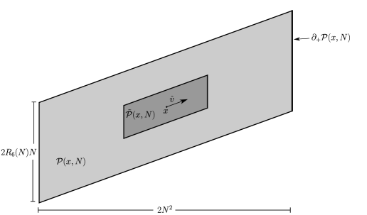
Figure 4: The set $\mathcal{P}(x,N)$ and its right boundary part $\partial_{+}\mathcal{P}(x,N)$ as well as its middle third $\tilde{\mathcal{P}}(x,N)$.

For $N\geq 1$, define the event

$$A_{N}(X):=\bigl{\{}X^{*(n)}<R_{2}(N)\ \forall n\in\{1,\ldots,2N^{2}\}\bigr{\}},$$

where at times we write $A_{N}$ instead of $A_{N}(X)$ if the corresponding process $X$ is clear from the context. Using Markov’s inequality, the following lemma is a consequence of Theorem 3.1.

Lemma 3.3

There exists a constant $C>0$ such that for each $N\geq 1$,

$$P_{0}(A_{N}^{c})\leq Ce^{-C^{-1}R_{2}(N)^{\gamma}}$$ (11)

and, defining the event

$$\mathcal{A}_{N}:=\bigcap_{x\in\tilde{\mathcal{P}}(0,N)}\bigl{\{}P_{x,\omega}(A_{N}^{c})\leq e^{-R_{1}(N)^{\gamma}}\bigr{\}},$$

which is contained in the Borel-$\sigma$-algebra of $\Omega$, one has

$$\mathbb{P}(\mathcal{A}_{N}^{c})\leq Ce^{-C^{-1}R_{2}(N)^{\gamma}}.$$

We define the set of rapidly decreasing sequences as

$$\mathcal{S}(\mathbb{N}):=\Bigl{\{}(a_{n})_{n\in\mathbb{N}}\in\mathbb{R}^{\mathbb{N}}\dvtx\sup_{n\in\mathbb{N}}|n^{k}a_{n}|<\infty\ \forall k\in\mathbb{N}\Bigr{\}}$$

and note that due to Lemma 3.3 we have that $N\mapsto P_{0}(A_{N}^{c})$ and $N\mapsto\mathbb{P}(\mathcal{A}_{N}^{c})$ are contained in $\mathcal{S}(\mathbb{N})$.

3.3 Berger’s semi-local limit theorem and scaling

As a first step in the scaling, we introduce a classification of blocks. We need to define some parameters which will remain fixed throughout this paper. For $\beta$ and $\alpha$ as in the assumptions of Proposition 2.1, choose $\delta$ such that

$$0<\delta<\frac{\beta d-\alpha}{12d}.$$

Furthermore, fix

$$\psi\in\biggl{(}2\delta,\frac{20\delta}{9}\biggr{)}$$ (12)

and $\chi$ such that

$$0<\chi<(\beta-6\delta)/2\wedge\psi/4\wedge 6/(d-1).$$

From now on let $L\in\mathbb{N}$, define $L_{1}:={\lfloor L^{\psi}\rfloor}$ and recursively in $k$ the scales

$$L_{k+1}:=L_{k}{\lfloor L^{\chi}\rfloor}.$$ (13)

Define $\iota$ to be the smallest $k$ such that $L_{k}^{2}>L^{1+\delta}$. For $k\in\{1,\ldots,\iota\}$ and $x\in C_{L}\cap\mathcal{L}_{L_{k}}$, we call a block

$${\mathcal{P}}(x,L_{k})$$ (14)

good with respect to the environment $\omega$ if the following three properties are satisfied for $\vartheta:=\chi$ and all $z\in\tilde{{\mathcal{P}}}(x,L_{k})$:

$$P_{z,\omega}\bigl{(}T_{\partial{\mathcal{P}}(x,L_{k})}\not=T_{\partial_{+}{\mathcal{P}}(x,L_{k})}\bigr{)}\leq e^{-R_{1}(L_{k})^{\gamma}}.$$ (15)

$$\bigl{\|}E_{z,\omega}\bigl{(}X_{T_{\partial{\mathcal{P}}(x,L_{k})}}|T_{\partial{\mathcal{P}}(x,L_{k})}=T_{\partial_{+}{\mathcal{P}}(x,L_{k})}\bigr{)}$$

(16)

$$\qquad{}-E_{z}\bigl{(}X_{T_{\partial{\mathcal{P}}(x,L_{k})}}|T_{\partial{\mathcal{P}}(x,L_{k})}=T_{\partial_{+}{\mathcal{P}}(x,L_{k})}\bigr{)}\bigr{\|}_{1}\leq R_{4}(L_{k}).$$

$$\max_{Q}\bigl{|}P_{z,\omega}\bigl{(}X_{T_{\partial{\mathcal{P}}(x,L_{k})}}\in Q|T_{\partial{\mathcal{P}}(x,L_{k})}=T_{\partial_{+}{\mathcal{P}}(x,L_{k})}\bigr{)}$$

$$\qquad{}-P_{z}\bigl{(}X_{T_{\partial{\mathcal{P}}(x,L_{k})}}\in Q|T_{\partial{\mathcal{P}}(x,L_{k})}=T_{\partial_{+}{\mathcal{P}}(x,L_{k})}\bigr{)}\bigr{|}$$ (17)

$$\qquad\quad<L_{k}^{(\vartheta-1)(d-1)-\vartheta({d-1})/({d+1})},$$

where the maximum in $Q$ is taken over all $(d-1)$-dimensional hypercubes $Q\subset\partial_{+}{\mathcal{P}}(x,L_{k})$ of side length $\lceil{L_{k}^{\vartheta}}\rceil$. Otherwise, we say that the block $\mathcal{P}(x,L_{k})$ is bad. For $k\in\{1,\ldots,\iota\}$ we will usually refer to boxes of the form ${\mathcal{P}}(x,L_{k})$ as a box of scale $k$.

The following result is essentially Proposition 4.5 of Be-09, which can be understood as a semi-local central limit theorem for RWRE. For the sake of completeness, we will give its proof in the Appendix.

Proposition 3.4 ((Proposition 4.5 of Be-09))

Assume that $(T)_{\gamma}|l$ is satisfied and fix $\vartheta\in(0,\frac{6}{d-1}\wedge 1)$. Then there exists a sequence of events $(G_{L})_{L\in\mathbb{N}}\subset\Omega$ such that $\mathbb{P}(G_{\cdot}^{c})\in\mathcal{S}(\mathbb{N})$ and for all $\omega\in G_{L}$ and $k\in\{1,\ldots,\iota\}$:

display (15),

display (3.3) and

display (3.3) are satisfied for all $x\in C_{L}\cap\mathcal{L}_{L_{k}}$, $z\in\tilde{{\mathcal{P}}}(x,L_{k})$ and the chosen $\vartheta$.

In particular, due to the translation invariance of the environment, we have that $\mathbb{P}(\mathcal{P}(x,\cdot)\mbox{ is bad})\in\mathcal{S}(\mathbb{N})$ for any $x\in\mathbb{Z}^{d}$.

Remark 3.5.

For the sake of notational simplicity, we will prove the proposition by showing that there exist sequences $G_{L}^{\mbox{\hyperlink{item:quenchedBadExitEst}{{(i)}}}}$, $G_{L}^{\mbox{\hyperlink{item:quenchedAnnealedExpDiff}{{(ii)}}}}$ and $G_{L}^{\mbox{\hyperlink{item:quenchedAnnealedProbDiff}{{(iii)}}}}$, $L\in\mathbb{N}$, of subsets of $\Omega$ such that

$$\mathbb{P}\bigl{(}{G_{L}^{\mbox{\hyperlink{item:quenchedBadExitEst}{{(i)}}}}}^{c}\bigr{)},\qquad\mathbb{P}\bigl{(}{G_{L}^{\mbox{\hyperlink{item:quenchedAnnealedExpDiff}{{(ii)}}}}}^{c}\bigr{)}\quad\mbox{and}\quad\mathbb{P}\bigl{(}{G_{L}^{\mbox{\hyperlink{item:quenchedAnnealedProbDiff}{{(iii)}}}}}^{c}\bigr{)}\vspace*{-1pt}$$

are contained in $\mathcal{S}(\mathbb{N})$ as functions in $L$ and such that for $\omega$ contained in these sets, $x=0$, and $z\in\tilde{\mathcal{P}}(0,L)$, displays (15), (3.3) and (3.3), respectively, are fulfilled for $L$ instead of $L_{k}$. The required result then follows by observing that $\mathbb{P}$ is translation invariant and using $|C_{L}|\leq CL^{2d}$ in combination with a standard union bound.

We next give an upper bound on the probability that an environment has many bad blocks. For this purpose, set

$$\Theta_{L}:=\bigl{\{}\omega\in\Omega\dvtx|\{x\in C_{L}\cap\mathcal{L}_{L_{k}}\dvtx{\mathcal{P}}(x,L_{k})$$

(18)

$$\hskip 77.3pt\mbox{ is bad with respect to }\omega\}|\leq L^{\alpha+\delta}\ \forall k\in\{1,\ldots,\iota\}\bigr{\}}.\vspace*{-1pt}$$

Furthermore, observe that $\mathcal{L}_{L}$ can be represented as the disjoint union of $2\cdot 8^{d-1}$ (translated) sublattices of $\mathbb{Z}^{d}$ such that for any sublattice $\mathcal{L}$ of these and $z_{1},z_{2}\in\mathcal{L}$, we have $\mathcal{P}(z_{1},L)\cap\mathcal{P}(z_{2},L)=\varnothing$.

Lemma 3.6 ((Lemma 5.1 of Be-09))

For $L$ large enough,

$$\mathbb{P}(\Theta_{L}^{c})\leq e^{-L^{\alpha}}.\vspace*{-3pt}$$

For $k\in\{1,\ldots,\iota\}$, set

$$J_{L_{k}}(\omega):=|\{z\in C_{L}\cap\mathcal{L}_{L_{k}}\dvtx{\mathcal{P}}(z,L_{k})\mbox{ is bad with respect to }\omega\}|\vspace*{-1pt}$$

and note that

$$\mathbb{P}(\Theta_{L}^{c})\leq\sum_{k=1}^{\iota}\mathbb{P}(J_{L_{k}}>L^{\alpha+\delta}).\vspace*{-1pt}$$ (19)

As in Be-09 we can write $J_{L_{k}}=J_{L_{k}}^{(1)}+\cdots+J_{L_{k}}^{(2\cdot 8^{d-1})}$ with $J_{L_{k}}^{(m)}$ distributed binomially with parameters $D({L_{k}})$ and $p({L_{k}})$ for $m\in\{1,\ldots,2\cdot 8^{d-1}\}$. Here, $p(L):=\mathbb{P}(\mathcal{P}(0,L)\mbox{ is bad})$, that is, in particular, due to Proposition 3.4,

$$p\in\mathcal{S}(\mathbb{N}),$$ (20)

and $D(L_{k})$ is the maximal number of intersection points any of the above-mentioned translated sublattices has with $C_{L}$, that is, in particular

$$D(L_{k})\leq CL^{2d}$$ (21)

for some constant $C$ and all $L$. Now for $m\in\{1,\ldots,2\cdot 8^{d-1}\}$, we have

$$\mathbb{P}\biggl{(}J_{L_{k}}^{(m)}>\frac{L^{\alpha+\delta}}{2\cdot 8^{d-1}}\biggr{)}\leq\exp\biggl{\{}-\frac{L^{\alpha+\delta}}{2\cdot 8^{d-1}}\biggr{\}}\mathbb{E}\exp\bigl{\{}J_{L_{k}}^{(m)}\bigr{\}}$$ (22)

with

$$\mathbb{E}\exp\bigl{\{}J_{L_{k}}^{(m)}\bigr{\}} \leq \sum_{j=0}^{D(L_{k})}\pmatrix{D({L_{k}})\cr j}(ep({L_{k}}))^{j}\bigl{(}1-ep({L_{k}})\bigr{)}^{D({L_{k}})-j}$$

$$\hskip 22.6pt{}\times\biggl{(}\frac{1-p({L_{k}})}{1-ep({L_{k}})}\biggr{)}^{D({L_{k}})-j},$$

and from (20) and (21) we conclude that

$$\lim_{L\to\infty}\biggl{(}\frac{1-p({L_{k}})}{1-ep({L_{k}})}\biggr{)}^{D({L_{k}})-j}=1$$

uniformly in $j\in\{0,\ldots,D(L_{k})\}$. Substituting this back into displays (3.3), (22) and (19), we conclude the proof.

We now need to recall the concept of closeness between two probability measures introduced in Be-09. Here and in the following, if $Z$ is a $d$-dimensional random variable defined on a probability space with probability measure $\mu$, we write $E_{\mu}Z:=\int Z\,d\mu$ and if $\mu$ is a measure on $\mathbb{R}^{d}$, then we write $E_{\mu}:=\int x\,d\mu$, whenever the integrals are well defined. Furthermore, we define its variance via $\operatorname{Var}Z:=E\|Z-EZ\|_{1}^{2}$ whenever this expression is well defined and correspondingly for a probability measure $\mu$ on $\mathbb{R}^{d}$ with appropriate integrability conditions we write $\operatorname{Var}_{\mu}$.

Definition 3.7.

Let $\mu_{1}$ and $\mu_{2}$ be two probability measures on $\mathbb{Z}^{d}$. Let $\lambda\in[0,1)$ and $K$ be a natural number. We say that $\mu_{2}$ is $(\lambda,K)$-close to $\mu_{1}$ if there exists a coupling $\mu$ of three random variables $Z_{1}$, $Z_{2}$ and $Z_{0}$ such that: [(a)]

μ∘Zj-1=μj for $j\in\{1,2\}$,

μ(Z1／=Z0)≤λ,

μ(∥Z0-Z2∥1≤K)=1,

EμZ1=EμZ0,

∑x∥x-EμZ1∥12⋅|