X-ray observations of cluster outskirts:
current status and future prospects.

Abstract

Past and current X-ray mission allow us to observe only a fraction of the volume occupied by the ICM. After reviewing the state of the art of cluster outskirts observations we discuss some important constraints that should be met when designing an experiment to measure X-ray emission out to the virial radius. From what we can surmise WFXT  is already designed to meet most of the requirements and should have no major difficulty in accommodating the remaining few.

1 Introduction

Galaxy clusters form through the hierarchical accretion of cosmic matter. The end products of this process are virialized structures that feature, in the X-ray band, similar radial profiles of the surface brightness $S_{\rm b}$ (e.g. Vikhlinin et al. 1999, Neumann 2005, Ettori & Balestra 2009) and of the plasma temperature $T_{\rm gas}$ (e.g. Allen et al. 2001, Vikhlinin et al. 2005, Leccardi & Molendi 2008). Such measurements have definitely improved in recent years thanks to the arcsec resolution and large collecting area of the present X-ray satellites, like Chandra and XMM-Newton, but still remain difficult, in particular in the outskirts, because of the low surface brightness associated to these regions. Present observations provide routinely reasonable estimates of the gas density, $n_{\rm gas}$, and temperature, $T_{\rm gas}$, up to about $R_{2500}$ ($\approx 0.3R_{200}$; $R_{\Delta}$ is defined as the radius of the sphere that encloses a mean mass density of $\Delta$ times the critical density at the cluster’s redshift; $R_{200}$ defines approximately the virialized region in galaxy clusters). Only few cases provide meaningful measurements at $R_{500}$ ($\approx 0.7R_{200}$) and beyond (e.g. Vikhlinin et al. 2005, Leccardi & Molendi 2008, Neumann 2005, Ettori & Balestra 2009). Consequently, more than two-thirds of the typical cluster volume, just where primordial gas is accreting and dark matter halo is forming, is still unknown for what concerns both its mass distribution and its thermodynamical properties. This poses a significant limitation in our ability to characterize the physical processes presiding over the formation and evolution of clusters and to use clusters as cosmological tools, as also outlined in the Scientific Justification for the WFXT (Giacconi et al. 2009). Indeed the characterization of thermodynamic properties at large radii would allow us to provide constraints on the virialization process, while measures of the metal abundance would allow us to gain insight on the enrichment processes occurring in clusters (e.g. Fabjan et al. 2010). Morever the X-ray emission at large radii could also be used to improve significantly measures of the gas and total gravitating masses thereby opening the way to a more accurate use of galaxy clusters as cosmological probes (e.g. Voit 2005).

In these proceedings, we take stock of the situation on cluster outskirts and suggest how to make progress. In Sect. 2, we provide an observational overview of currently available measures of cluster outer regions, while in Sect. 3 we discuss some important constraints that should be met when designing an experiment to measure X-ray emission out to the virial radius. In Sect. 4, we present an overview of future missions which have cluster outskirts observations as one of their goals, our main results are recapitulated in Sect. 5.

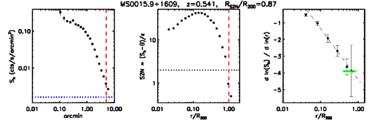
Figure 1: From left to right: Example of a surface brightness profile with the fitted background (horizontal dotted line) and the radius $R_{200}$ (vertical dashed line); the signal-to-noise profile evaluated as $S2N=(S_{b}-B)/\epsilon$, where the error $\epsilon$ is the sum in quadrature of the Poissonian error in the radial counts and the uncertainties in the fitted background, $B$; the best-fit values of the slope of the surface brightness profile as a function of $r/R_{200}$. These values are estimated over 6 radial bins (thick horizontal solid line: the slope evaluated between $0.4\times R_{200}$ and $R_{S2N}$ with a minimum of 3 radial bins; dashed line: best-fit of $d\ln(S_{b})/d\ln(r/R_{200})$ with the functional form $s_{0}+s_{1}\ln(r/R_{200})$ over the radial range $0.1\times R_{200}-R_{S2N}$, with the best-fit parameters quoted in Table 3 of Ettori & Balestra 2009).

A Hubble constant of 70 $h_{70}$ km s^-1 Mpc^-1 in a flat universe with $\Omega_{\rm m}$ equals to 0.3 is assumed throughout this manuscript.

2 What we know of cluster outskirts

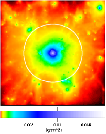
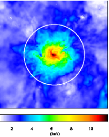
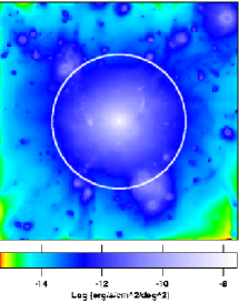
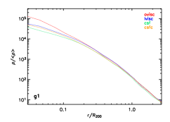
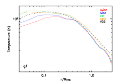
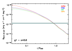
Figure 2: From left to right; upper panels: Maps of the projected gas density, mass-weighted temperature and soft (0.5-2 keV) X-ray emission. The circles indicate the virial radius. The size of the side of each map is 12 Mpc, so they cover roughly up to $2.5R_{200}$. Bottom panels: Comparison between the gas density, mass-weighted temperature, soft X-ray surface brightness profiles for a cluster with $M_{\rm vir}~{}2\times 10^{15}M_{\odot}$ simulated by using 4 different physical models (Roncarelli et al. 2006). A dashed line indicates the functional from Vikhlinin et al. (2006, eq. 9) that well reproduces the behavior of the temperature profile of nearby bright galaxy clusters observed with Chandra. The extragalactic unresolved background from Hickox & Markevitch (2006) in the soft X-ray band is indicated by the shaded region.

2.1 Surface brightness and gas density profiles

The X-ray surface brightness is a quantity much easier to characterize than the temperature and it is still rich in physical information being proportional to the emission measure, i.e. to the gas density, of the emitting source. Recent work focused on a few local bright objects for which ROSAT PSPC observations with low cosmic background and large field of view have allowed to recover the X-ray surface brightness profile over a significant fraction of the virial radius (Vikhlinin et al. 1999, Neumann 2005).

In Ettori & Balestra (2009), we study the surface brightness profiles extracted from a sample of hot ($T_{\rm gas}>3$ keV), high-redshift ($0.3<z<1.3$) galaxy clusters observed with Chandra and described in Balestra et al. (2007). A local background, $B$, was defined for each exposure by considering a region far from the X-ray center that covered a significant portion of the exposed CCD with negligible cluster emission. We define the “signal-to-noise” ratio, $S2N$, to be the ratio of the observed surface brightness value in each radial bin, $S_{b}(r)$, after subtraction of the estimated background, $B$, to the Poissonian error in the evaluated surface brightness, $\epsilon_{b}(r)$, summed in quadrature with the error in the background, $\epsilon_{B}$: $S2N(r)=\left[S_{b}(r)-B\right]/\sqrt{\epsilon_{b}(r)^{2}+\epsilon_{B}^{2}}$. The outer radius at which the signal-to-noise ratio remained above $2$ was defined to be the limit of the extension of the detectable X-ray emission, $R_{S2N}$. We estimated $R_{200}$ using both a $\beta-$model that reproduces the surface brightness profiles and the scaling relation quoted in eq. 1 and selected the 11 objects with $R_{S2N}/R_{200}>0.7$ to investigate the X-ray surface-brightness profiles of massive clusters at $r>R_{500}\approx 0.7R_{200}$. Examples of the analyzed dataset are shown in Fig. 1. We performed a linear least-squares fit between the logarithmic values of the radial bins and the background-subtracted X-ray surface brightness. Overall, the error-weighted mean slope is $-2.91$ (with a standard deviation in the distribution of $0.46$) at $r>0.2R_{200}$ and $-3.59(0.75)$ at $r>0.4R_{200}$. For the only 3 objects for which a fit between $0.5R_{200}$ and $R_{S2N}$ was possible, we measured a further steepening of the profiles, with a mean slope of $-4.43$ and a standard deviation of $0.83$. We also fitted linearly the derivative of the logarithm $S_{b}(r)$ over the radial range $0.1R_{200}-R_{S2N}$, excluding in this way the influence of the core emission. The average (and standard deviation $\sigma$) values of the extrapolated slopes are then $-3.15(0.46)$, $-3.86(0.70)$, and $-4.31(0.87)$ at $0.4R_{200}$, $0.7R_{200}$ and $R_{200}$, respectively.

These values are comparable to what has been obtained in recent analyses. Vikhlinin et al. (1999) find that a $\beta-$model with $\beta=0.65-0.85$ describes the surface brightness profiles in the range $0.3-1R_{180}$ of 39 massive local galaxy clusters observed with ROSAT PSPC. For a $\beta-$model with $x=r/r_{\rm c}$, $\partial\ln S_{b}/\partial\ln x=(1-6\beta)\,x^{2}/(1+x^{2})$ and $\partial\ln n_{\rm gas}/\partial\ln x=-3\beta\,x^{2}/(1+x^{2})$, impling that $\beta=0.65-0.85$ corresponds to a logarithmic slope of the surface brightness of $-2.9/-4.1$, that is a range that includes our estimates. Neumann (2005) finds that the stacked profiles of few massive nearby systems located in regions at low ($<6\times 10^{20}$ cm^-2) Galactic absorption observed with ROSAT PSPC still provide values of $\beta$ around $0.8$ at $R_{200}$, with a power-law slope that increases from $-3$ when the fit is performed over the radial range $[0.1,1]R_{200}$ to $-5.7^{+1.5}_{-1.2}$ over $[0.7,1.2]R_{200}$.

These observational results are supported from the hydrodynamical simulations of X-ray emitting galaxy clusters performed with the Tree+SPH code GADGET-2 (Roncarelli et al. 2006; see, e.g., Fig. 2). In the most massive systems, we measured a steepening of $S_{b}(r)$, independently from the physics adopted to treat the baryonic component, with a slope of $-4,-4.5,-5.2$ when estimated in the radial range $0.3-1.2R_{200}$, $0.7-1.2R_{200}$, $1.2-2.7R_{200}$, respectively. In particular, we note the good agreement between the slope of the simulated surface brightness profile of the representative massive cluster in the radial bin $0.7-1.2R_{200}$ (see values of $b_{A}$ in Table 4 of Roncarelli et al. 2006 ranging between $-4.29$ and $-4.54$) and the mean extrapolated value at $R_{200}$ of $-4.43$ measured in the Chandra dataset.

2.2 Temperature and metallicity profiles

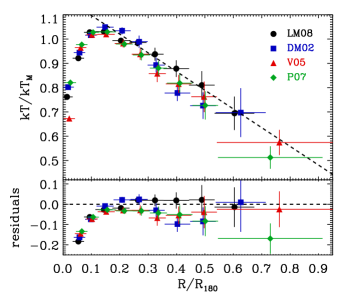
Figure 3: Left panel: mean temperature profiles obtained from Leccardi & Molendi (2008; LM08, black circles), De Grandi & Molendi (2002; DM02, blue squares), Vikhlinin et al. (2005; V05, red upward triangles) and Pratt et al. (2007; P07, green diamonds). All profiles are rescaled by $\mathrm{k}T_{\mathrm{M}}$ and $R_{180}$. The dashed line shows the best fit with a linear model beyond 0.2 $R_{180}$ and is drawn to guide the eye. lower panel: residuals with respect to the linear model. The LM08 profile is the flattest one. Right panel: mean metallicity profiles obtained from Leccardi & Molendi (2008b; LM08, circles), De Grandi et al. (2004; DM04, triangle) and Baldi et al. (2007; BA07, squares). Abundances are expressed in Anders & Grevesse (1989) solar values and radii in units of $R_{180}$. The radii have been slightly offset in the plot for clarity.

Early attempts to produce temperature profiles were made with the ROSAT PSPC, these were mostly limited to low mass systems (e.g. David et al. 1996) where the temperatures were within reach of the PSPC soft response. Resolved spectroscopy of hot systems began with the coming into operation of ASCA (1994) and BeppoSAX (1996). Both missions enjoyed a relatively low instrumental background, which was a considerable asset when extending measures out to large radii, however they both suffered from limited spatially resolution. The situation was somewhat less severe with the BeppoSAX MECS than with the ASCA GIS since the former had a factor of 2 better angular resolution and a modest energy dependence in the PSF. These difficulties led to substantial differences in temperature measures, while on the one side Markevitch et al. (1998) using ASCA  and De Grandi & Molendi (2002) using BeppoSAX MECS found evidence of declining temperature profiles, on the other, White (2000) using ASCA and Irwin et al. (1999) using BeppoSAX data found flat temperature profiles. The situation was somewhat clearer on abundance profiles were workers using ASCA (e.g. Finoguenov et al. 2000) and BeppoSAX data (De Grandi & Molendi 2001) consistently found evidence that cool core systems featured more centrally peaked profiles than NCC system. The coming into operation of the second generation of medium energy X-ray telescopes, namely XMM-Newton and Chandra, both characterized by substantially better spatial resolution, allowed more direct measures of the temperature profiles. The new Chandra (Vikhlinin et al. 2005) and XMM-Newton measurements (e.g. Pratt et al. 2007, Snowden et al. 2008) confirmed the presence of the temperature gradients measured with ASCA and BeppoSAX. In a detailed study of a sample of 44 objects observed with XMM-Newton (Leccardi & Molendi 2008) we found that temperature measurements could be extended out to about 0.7$R_{180}$ (see Fig. 3). Since the major obstacle to the extension of measurements to large radii was the high background, most importantly the instrumental component, we adopted the source over background criterion originally introduced in De Grandi & Molendi (2002) to decide where to stop measuring profiles. The source to background ratio, defined as ${I_{sou}\over I_{bkg}}$, where $I_{sou}$ and $I_{bkg}$ are the source and background intensities respectively, should not be confused with the signal to noise ratio defined as ${I_{sou}\over(I_{sou}+I_{bkg})^{1/2}}\cdot t$, where $t$ is the exposure time. While the latter ratio is associated to the statistical error and therefore increases with exposure time, the former is associated to the systematic error and does not depend on the exposure time. Through a series of tests (see Sect. 5.2.1. and Fig. 11 of Leccardi & Molendi 2008) we determined that measurements could be trusted out to radii where the source to background ratio in the 0.7-10 keV band remained above a threshold of 0.6. In Leccardi & Molendi (2008) we made use for the first time of extensive simulations to estimate the impact of systematic errors on the measurements, part of the expertise we have acquired from that work has been used to perform the simulations discussed in Sect. 3.4. In the left panel of Fig. 3 we show a compilation of mean temperature profiles from different missions, all show evidence of a decline of the temperature beyond 0.2$R_{180}$. Interestingly, as a result of the correction for systematic that we applied to our profile (see Sect. 5.3 and Fig. 14 of Leccardi & Molendi 2008) ours is the flattest amongst the profiles shown in the left panel of Fig. 3. The measurement of the metal abundance profile extends to radii that are somewhat smaller than those reached by the temperature profiles, this is because the most prominent emission line, the Fe K$\alpha$, is located in the high energy part of the spectrum where the instrumental background is particularly strong. In the right panel of Fig. 3 we show the mean abundance profile measured with different satellites. The flattening of the profiles beyond 0.2$R_{180}$ is most likely indicative of an early enrichment of the ICM (Fabjan et al. 2010).

Unfortunately the high orbit of the XMM-Newton and Chandra satellites, as well as the fact that the design of the satellites was driven by scientific objectives other than the characterization of low surface brightness regions, led to a substantially higher and more variable background than with the previous satellite generation, thereby limiting the exploration of the temperature and abundance profiles to roughly the same regions already investigated with ASCA and BeppoSAX (see Fig. 3). Recently measures of temperature profiles have been made with the Suzaku X-ray imaging spectrometer (XIS). Although not ideal for cluster measurements, the XIS features a poor PSF and a small FOV, it does enjoy the considerable advantage of the modest background associated to the low earth orbit. The measures have been conducted on a handful of systems (A2204, Reiprich et al. 2009; A1795, Bautz et al. 2009; PKS0745-191, George et al. 2009; A1413, Hoshino et al. 2010) and extend beyond the regions explored with Chandra and XMM-Newton. However, the characterization is a limited one at best: only parts of the outermost annuli are explored and both radial bins and error bars are large. Moreover there are concerns as to the reliability of the measurements themselves. All measured temperature profiles are steeper than those predicted by simulations. This is particularly true of A1795 and PKS0745-191, where the temperature and the surface brightness are respectively steeper and flatter than those predicted by simulations. Consequently entropy profiles are flatter and, in the case of PKS0745-191, it features an inversion around $0.6R_{200}$, that could be associated to the presence of non virialized gas or, alternatively, to problems in the characterization of the source spectrum.

3 How we can map out to $R_{200}$

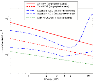
Figure 4: Left panel: compilation of instrumental background spectra, only continuum components, for various X-ray missions equipped with CCD detectors from Hall et al. (2008). Right panel: Resolved fraction of extragalactic cosmic X-ray background in the 0.5–2 keV band as a function of angular resolution.The total background intensity is derived from measures by De Luca & Molendi (2004) and Mc Cammon et al. (2002). The LogN-logS is taken from Moretti et al. (2003). We also include an euclidian component to account for the unresolved 20% of the cosmic X-ray background (CXB). The normalization of this component is conservatively chosen in such a way that about 10% of the CXB is found at fluxes that are sufficiently small to efficiently mimic a diffuse component. The angular resolution necessary to reach a given flux limit is obtained by imposing that the source density at that flux limit is such that there is 1 source every 20 angular resolution elements, where the angular resolution element is a circle with a radius equal to the half-power-radius of the PSF.

From the discussion in Sect. 2.2, it is rather obvious that past X-ray mission were not optimized for the spectral characterization of the low surface brightness emission typical of cluster outer regions. In this section we discuss how to design an experiment characterized by high sensitivity to low surface brightness emission. The sensitivity depends upon: 1) the surface brightness of the source, $S_{b}$, that scales with effective area of the experiment, $A_{E}$; 2) the solid angle covered by the field of view (FOV), $\Omega$; 3) the surface brightness of the background, $B$. The quantity that needs to be maximized is then:

$$s={2\pi\int_{0}^{\theta_{max}}A_{E}(\theta)\theta d\theta\over B},$$

where $\theta$ is the off-axis angle and the integration is extended over the full FOV, i.e. $2\pi\int_{0}^{\theta_{max}}\theta d\theta=\Omega$. Therefore one needs to maximize the numerator, $2\pi\int_{0}^{\theta_{max}}A_{E}(\theta)\theta d\theta$, a quantity that is often referred to as “grasp”, and minimize the background . To go well beyond what has been achieved with the instrumentation that has been designed thus far one needs to operate at three different levels: 1) the experiment design; 2) the observational strategy; 3) the data analysis strategy.

3.1 Experiment design

Let us start by considering the background and in particular the instrumental background, i.e. the part of the background that is not associated to genuine cosmic X-ray photons. A few things can be easily inferred by comparing background spectra from different mission. In Fig. 4 we report a recent compilation of such spectra from Hall et al. (2008). We note that: 1) front illuminated CCDs have lower background than background illuminated ones and that 2) the background on the low earth orbit is smaller than that in the high orbit. In this respect it is particularly instructive to compare the EPIC MOS with the SWIFT XRT background, since we are dealing with virtually the same detector in a high and low earth orbit. As shown in Hall et al. (2008), the SWIFT XRT background is about a factor 3 lower than the EPIC MOS background. Thus, from the inspection of Fig. 4 we learn that to keep the instrumental background low it is preferable to employ front illuminated CCDs on a low earth orbit. There are other issues that should be kept in mind: 1) a non-negligible fraction (say 15%) of the detector should be shielded from the sky, this will allow to constantly monitor the intensity of the instrumental background; 2) a tilted CCD configuration which allows to improve the imaging, will result in fluorescence Si line emission inhomogeneous distributed on the FOV, something similar is observed on MOS EPIC, this can be minimized by studying the most appropriate configuration; 3) while active shielding cannot be applied as long as the detector is a CCD, passive shielding can and should be considered. Most importantly the whole instrumental background issue should be addressed from a global point of view. Detailed simulations of the physical interaction between particles and photons with the satellite, possibly complemented by exposures of the detector and associated structures to real particles and high energy photons, can be used to study solutions that will minimize the background.

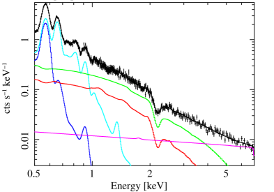
Figure 5: Simulation of source and background spectra for a typical region at R200. Tne instrumental background estimates come from current missions. The cosmic X-ray background (CXB) is modeled with 3 components, for the soft X-ray background (SXRB) we adopt the modeling of the SXRB from McCammon et al. (2002), who have carried out the highest spatial resolution observation of the SXRB with a sounding rocket flight. The SXRB is modeled by 2 thermal components with temperatures of 0.1 keV and 0.225 keV both with solar abundances, normalizations come from Table 3 of McCammon et al. (2002). For the extragalactic background, comprising mostly unresolved AGNs, we assume a power-law of slope 1.4 and intensity 1/4 of that derived by De Luca & Molendi (2004), thereby assuming that 3/4 of the sources will be resolved out. The source surface brightness is assumed to be $3\times 10^{-16}$ erg cm^-2s^-1arcmin^-2, a typical value for cluster outskirts (see Sect. 2.1 for a detailed discussion), the extraction region is 100 arcmin², a value of $2\times 10^{20}$cm^-2 is assumed for the equivalent hydrogen column density, the cluster emission is modeled by a thermal plasma with kT$=$3 keV and metal abundance Z$=$0.15 Z_⊙, the exposure time was set to 100 ks. The model spectrum was convolved with response files (effective are and redistribution matrix) provided by the WFXT team.

If the experiment is properly designed then the instrumental background will be low and the cosmic background important. Above $\simeq$ 1 keV the dominant contributor to the cosmic X-ray background is the extragalactic background associated to unresolved sources, mostly AGN. Sufficiently high spatial resolution allows to resolve out a sizeable fraction of the sources producing the X-ray background (see Fig. 4b). With a resolution of 5 arcsec (Half-Power-Ratio, HPR) it is possible to resolve out about 80% of the background, provided of course sufficient counts are available to detect the sources. It should be noted that beyond an angular resolution of 15 arcsec the resolved fraction is not very sensitive to the resolution, see Fig. 4b. Another important point is that, to fully exploit the advantage of a large field of view, it is necessary that the high spatial resolution be available over the full FOV, polynomial optics (Burrows et al. 1992) can provide this important feature. Another important contributor to the background is the so called straylight, this is associated to X-ray photons from outside the field of view which end up in the focal plane after reflecting only once on the mirrors. The effect of straylight can be significantly mitigated by introducing a pre-collimator in front of the telescope as was done in the case of the XMM-Newton optics.

3.2 Observing and data analysis strategies

An experiment design like the one described above contributes significantly in improving the sensitivity to low surface brightness emission, however further steps need to be taken to reach cluster outer regions. This is quite apparent when looking at the spectral simulation reported in Fig. 5 (for details see the figure caption). As can be seen background components of one kind or another dominate the spectrum at all energies. In the 1-3 keV range the source intensity is about 1/3 of the total, below 1 keV the galactic foreground dominates, while above 3 keV the residual extragalactic and the instrumental background do. These are of course estimates, for real clusters things may be a little different, however we will inevitably have a background that outshines the source. These are atypical conditions with respect to previous X-ray imaging missions. To make reliable measures will require devising specific observing and analysis strategies. Clearly the strongest requirement is that the background be characterized as well as possible, ideally one would like to measure the background associated to the source without the source, which is of course impossible. Considering that the instrumental component varies with time and that the galactic foreground varies with position on the sky, it is important to observe the background almost at the same time and almost at the same location of the source. A similar strategy has been adopted, albeit for reasons different from the ones considered here, by the SWIFT XRT experiment. During each 1.5 hour orbit, SWIFT observes a source field and 3 or 4 background fields. Thus background fields are observed almost simultaneously with the source field and with the same instrument set up. Moretti et al. (2010) have shown that under these conditions the instrumental background can be characterized to the 3% level. Conversely, when background fields from different epochs are used, only a 10-15% level is achieved. The optimal solution that may be applied in a future mission, or on SWIFT for that matter, would be to use as part of the background fields, sky regions close to the source and dark earth observations. The former would allow to perform a spatial characterization of the galactic foreground, while the latter would permit a clean measurement of the instrumental background. Observations of both source and background fields need to be conducted to a high precision. Relative systematic errors on the spectra need to be kept at the few percent level. This is not a trivial requirement to meet, particularly since at this level of precision each detector element has to be considered as an independent detector. Assuming that each detector element will be calibrated to a relative precision of $\simeq 5\%$, systematics can be reduced to the desired level by viewing each sky element with a large number of detector elements. Observing strategies such as this have been used for decades in other bands of the electromagnetic spectrum when the source signal is smaller than the background. As examples, one may consider ground based infrared observations or cosmic microwave background measurements.

The comparison of the source plus background spectrum with the background spectrum is typically done via subtraction. In recent years, workers concentrating on cluster outer regions (e.g. Snowden et al. 2008, Leccardi & Molendi 2008) are finding that modeling is more effective. This is readily understood if one considers that the background is made of different components each capable of varying independently of the others. Unless there are good reasons to believe that the particular combination of background components associated to the source and background fields are next to identical, it is preferable to model the different components allowing for variations in relative intensity. Another issue that should be considered is that, under the atypical conditions of cluster outer regions, the standard maximum likelihood estimators commonly employed to derive physical parameters such as emission measure and temperature do not always work properly. In a recent paper (Leccardi & Molendi 2007), we have shown that the presence of a significant background component can lead to a substantially biased measure of the temperature. In the same paper, we describe a few quick fixes. Unfortunately, a general solution, based on a more powerful statistical estimator, has yet to be found.

3.3 A budget for systematics

Assuming that the above guidelines are followed, we expect to be able to maintain systematic errors to within a few percent. In the following, we provide a breakdown of the expected errors. A constant monitoring of the instrumental background by using the part of the detector not exposed to the sky plus dark earth and background field observations entwined with source observations should allow us to constrain this component to about 1% (as extrapolated from the results obtained on SWIFT XRT in Moretti et al. 2010). The extragalactic component of the cosmic background is a residual component, comprising unresolved sources and possibly a diffuse component. For a typical flux limit of 10^-16 erg cm^-2s^-1 in the 0.5-2.0 keV band, montecarlo simulations show that the cosmic variance for a 100 arcmin² field is less than 1% of the residual background component. The galactic foreground will be monitored by performing observations of fields contiguous to the source field. Moreover, observations over several 100 arcmin² should allow us to characterize this component to about 3-5%. Finally, assuming a typical relative calibration accuracy of 5% on individual detector elements and the application of substantial dithering, we expect to reach an overall relative spectral calibration of about 1%.

3.4 Detailed predictions

Table 1: Relative errors (in percentage) and deviations $\epsilon$ from the input values at 90% confidence level on the parameters of interest (normalization $K$, plasma temperature $T$ and metal abundance $Z$ of an apec component in XSPEC –Arnaud 1996) after joint-fit analysis of spectra simulated with an exposure time of 50 ksec. All the relative errors can be rescaled to different exposure times as $\sim\sqrt{t_{\rm exp}}$. $\beta_{20}$ indicates a $\beta$ value increased by 20 per cent. CC (nCC) indicates a (no) Cooling-Cores Cluster. The fluxes $f$ are in units of $10^{-12}$ erg/s/cm² in the band $(0.1-2.4)$ keV and are collected from http://bax.ast.obs-mip.fr/.

inputs		$K$	$T$		$K$	$T$	$Z$
		fixed $Z$
Perseus (TURBOLENT/CC; $z=0.0178,f=1137.3,T=6.3{\rm keV},n_{\rm H}=1.5e21;R_{200}=1.9{\rm Mpc}=88.2^{\prime}$)
$T=3.16,Z=0.15$		8 $(+0.2\epsilon)$	15 $(+0.5\epsilon)$		16 $(+0.3\epsilon)$	17 $(-1.3\epsilon)$	$>$100
$T=2,Z=0.15$		8 $(-1.0\epsilon)$	8 $(+0.7\epsilon)$		17 $(-0.1\epsilon)$	13 $(-0.4\epsilon)$	44 $(-0.2\epsilon)$
$\beta_{20},T=3.16,Z=0.15$		27 $(+1.1\epsilon)$	38 $(-0.7\epsilon)$		66 $(+0.4\epsilon)$	55 $(-1.4\epsilon)$	$>$100
$\beta_{20},T=2,Z=0.15$		25 $(+1.3\epsilon)$	30 $(+0.3\epsilon)$		51 $(+0.9\epsilon)$	47 $(-0.2\epsilon)$	5 $(-1.0\epsilon)$
A1689 (MERGING/nCC; $z=0.1810,f=14.5,T=10.1{\rm keV},n_{\rm H}=1.8e20;R_{200}=2.2{\rm Mpc}=12.2^{\prime}$)
$T=5.05,Z=0.15$		6 $(-0.7\epsilon)$	23 $(+0.5\epsilon)$		20 $(-0.9\epsilon)$	27 $(+1.1\epsilon)$	$>$100
$T=2,Z=0.15$		6 $(+0.1\epsilon)$	7 $(<0.1\epsilon)$		13 $(+0.2\epsilon)$	6 $(-3.2\epsilon)$	35 $(-1.3\epsilon)$
$\beta_{20},T=5.05,Z=0.15$		$>$100	$>$100		$>$100	$>$100	$>$100
$\beta_{20},T=2,Z=0.15$		55 $(+0.2\epsilon)$	14 $(-3.7\epsilon)$		$>$100	$>$100	$>$100

Our goal is to resolve the physical properties of the ICM in the virial regions making proper use of the WFXT (FOV with $R_{\rm WF}\approx 30^{\prime}$).

Our strategy is to define a set of observations with reasonable exposure time ($\leq$ 50 ksec) that can allow the study of the virial regions through the spatial and spectral analysis with WFXT.

First, we select objects with known X-ray properties (flux, temperature, dynamical status) that can be good candidates for a single WFXT exposure, i.e. with an expected $R_{200}<R_{\rm WF}=30^{\prime}$. We can also relax a bit this assumption requiring however that a given exposure minimizes the risks in term of (i) problems of intercalibration with other X-ray observatories for measurements in known X-ray emitting regions, (ii) weak constraints on the X-ray properties at $R_{200}$ due to the effect of unexpected large scale structures.

We estimate $R_{200}$ from a given spectroscopic measurement of the gas temperature by using the best-fit results in Arnaud et al. (2005, cf. Table 2; similar results in Vikhlinin et al. 2006):

$$R_{200}=1714\times(T_{\rm gas}/{\rm 5keV})^{0.5}\,E_{z}^{-1}h_{70}^{-1}\,{\rm kpc}$$ (1)

with $E_{z}=\left[\Omega_{\rm m}(1+z)^{3}+\Omega_{\Lambda}\right]^{0.5}$ and $\Omega_{\rm m}=1-\Omega_{\Lambda}=0.3$.

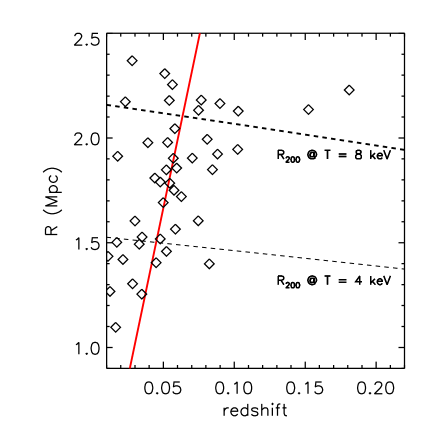
Figure 6: Predicted $R_{200}$ for the 45 objects in Mohr et al. (1999) compared to $R_{\rm WF}=30^{\prime}$ (red solid line) and the expected $R_{200}$ for a typical cluster with a temperature of 4 and 8 keV (dashed lines). $R_{200}$ are estimated from eq. 1.

By applying the criterion $R_{200}<R_{\rm WF}=30^{\prime}$, we select 23 out of the 45 objects present in the flux-limited sample of the brightest clusters in Mohr et al. (1999; see Fig. 6)). More objects can be included if off-axis exposures are considered, as requested for the Perseus cluster with a $R_{200}$ of $\sim 88$ arcmin.

The response matrix used for our simulations is obtained by convolving the redistribution matrix with a mean effective area, $\overline{A(E)}$, constructed by averaging the vignetting over the whole field of view, i.e.

$$\overline{A(E)}=A_{o}(E)\cdot{2\pi\int_{0}^{\theta_{max}}\theta~{}d\theta~{}V(E,\theta)\over\pi\theta_{max}^{2}},$$

where $A_{o}(E)$ is the energy dependent on-axis effective area, $\theta_{max}$ is maximum off-axis angle and $V(E,\theta)$ is the energy and off-axis dependent vignetting. The redistribution matrix, the on-axis effective area and the vignetting were kindly provided by the WFXT team. We use our own script with the response matrix to simulate a (source$+$background) and a (background only) spectrum including in the latter one (i) a 1 per cent random fluctuation in absorbing $n_{\rm H}$ value and in the normalization of the instrumental background; (ii) a 5 per cent random fluctuation propagated to the normalization and temperature values of the two local background component (one absorbed, the other not), to the normalization and photon-index value of the CXB. The photon-index is allowed to vary between $1.4$ and $1.6$. We assume that 80 per cent of the CXB is resolved.

The spectra are integrated for 50 ksec over an area of 100 arcmin² and then jointly fitted in the range $0.3-6$ keV.

The surface brightness in the band $(0.5-2)$ keV are obtained from the best-fit values in Table 2 of Mohr et al. (1999) by evaluating the model prediction at $R_{200}$ as estimated in equation 1. A more conservative estimate of the surface brightness is obtained by increasing the $\beta$ value by 20 per cent, faking an expected steepening of the surface brightness profile in the cluster outskirts, as recent observations and simulations suggest (see Section 2). This correction reduces the predicted surface brightness by a factor of 7 on average.

All the simulated spectra assume a metallicity of $0.15Z_{\odot}$ and a temperature equal to 0.5 (see Roncarelli et al. 2006) times the quoted value in Table 1 of Mohr et al. (1999). We also consider the cases with metallicity equal to $0.05Z_{\odot}$ and temperature of about 0.25 times the quoted values (i.e. between 1 and 2 keV).

Our simulated spectra (e.g. Fig. 5) show that we can reach typical uncertainties (90% level of confidence) of $\leq$ 20% on the normalization $K$ and temperature $T$ of the thermal spectra (see Tab. LABEL:tab:feasi). Reasonable constraints ($\sim$ 40%) on the metallicity $Z$ can be obtained in the case the surface brightness profile in the outskirts is still well reproduced from the models fitted to ROSAT PSPC data.

A steepening of the surface brightness profiles, as expected from the work discussed in Sect. 2 and modeled here by increasing the value of the outer slope $\beta$ by 20 %, reduces significantly the level of accuracy to which we can constrain the physical parameters: about 60 per cent (relative error at 90% level of confidence) on $K$, 40 per cent on $T$, no constraints on $Z$.

4 Future missions & WFXT

In this section we provide an overview of missions under study or construction that may provide important contributions to the characterization of cluster outer regions. There are 3 such missions namely SRG, XENIA and WFXT. The eROSITA experiment (Predehl et al. 2007) on board the Russian Spektrum Roentgen Gamma (SRG) satellite comprises 7 telescopes with a total on-axis effective area of 2000 cm², an on-axis angular resolution of 25 arcsec and will operate from an L2 orbit. XENIA (Hartmann et al. 2009) carries an X-ray imager and spectrometer that would both be useful in characterizing cluster outskirts: the imager has an on-axis effective area of 600 cm² and an on-axis angular resolution of 15 arcsec; the spectrometer has an unprecedented spectral resolution of a few eV, an on-axis effective area of about 1000 cm² and an angular resolution that is limited by the pixel size of a few arcmin. WFXT (Murray et al. 2010) which, like XENIA, has been submitted to the Astro2010: The Astronomy and Astrophysics Decadal Survey, carries an X-ray imager comprising 3 telescopes for a total on-axis effective area of 6000 cm², and an on-axis angular resolution of 5 arcsec (requirement for the half-power-radius of the PSF). A low earth equatorial orbit is forseen for both XENIA and WFXT.

Both the XENIA and WFXT imager have two considerable advantages over eROSITA, namely the low earth over the L2 orbit and the polynomial optics, which will result in a substantial reduction of the instrumental and cosmic X-ray background, respectively. In particular, the WFXT imager will provide the characterization of the cluster outer regions in about 1/10 of the time requested from XENIA, and will benefit from higher angular resolution. XENIA  however, is in the unique position to complement the imager data with high spectral resolution data for relatively bright clusters. While eROSITA is scheduled for launch in 2012, XENIA and WFXT are both at an early stage of development and have to be considered as the next generation satellites for clusters studies.

5 Summary

Past and current X-ray mission allow us to observe only a fraction of the volume occupied by the ICM. Indeed, typical measures of the surface brightness, temperature and metal abundance extend out to a fraction of the virial radius. The coming into operation of the second generation of medium energy X-ray telescopes at the turn of the millennium, has resulted in relatively modest improvements in our ability to characterize cluster outskirts. Even though recent results from Suzaku show some improvement, the most sensitive instrument to low surface brightness to have flown thus far is quite possibly the SWIFT XRT which, ironically, never had cluster outer regions as one of its top scientific objectives.

The construction of an experiment capable of making measures out to $R_{200}$ is well within the reach of currently available technology. What is required is an experiment design that will minimize the background, both instrumental and cosmic, and maximizes the grasp, i.e. the product of effective area and FOV. Since cluster emission in the outskirts will be background dominated, instrument design and observational strategy should also allow for a meticulous characterization of the background. Detailed simulations based on realistic estimates of the different spectral components and of the precision with which the may be determined shows that an experiments such as the one we envisage will allow a solid characterization of cluster outskirts. From what we can surmise WFXT is already designed to meet most of the requirements which are necessary to characterize cluster outskirts, and should have no major difficulty in accommodating the remaining few.

References

- Allen et al. (2001) Allen S.W., Schmidt R.W., Fabian A.C. 2001, MNRAS, 328, L37
- Anders & Grevesse (1989) Anders E., Grevesse N. 1989, Geochimica et Cosmochimica Acta, 53, 197
- Arnaud (1996) Arnaud K.A. 1996, Astronomical Data Analysis Software and Systems V, eds. Jacoby G. and Barnes J., p17, ASP Conf. Series volume 101
- Arnaud et al. (2005) Arnaud M., Pointecouteau E., Pratt G.W. 2005, A&A, 441, 893
- Balestra et al. (2007) Balestra I. et al. 2007, A&A, 462, 429
- Baldi et al. (2007) Baldi A. et al. 2007, ApJ, 666, 835
- Bautz et al. (2009) Bautz M.W. et al. 2009, PASJ, 61, 1117
- Burrows et al. (1992) Burrows et al. 1992, ApJ, 392,760
- David et al. (1996) David L.P. et al. 1996, ApJ, 473, 692
- De Grandi & Molendi (2001) De Grandi S., Molendi S. 2001, ApJ, 551, 153
- De Grandi & Molendi (2002) De Grandi S., Molendi S. 2002, ApJ, 567, 163
- De Grandi et al. (2004) De Grandi S. et al. 2004, A&A, 419, 7
- De Luca & Molendi (2004) De Luca A., Molendi S., 2004, A&A, 419, 837
- Ettori & Balestra (2009) Ettori S., Balestra I. 2009, A&A, 496, 343
- Fabjan et al. (2010) Fabjan D. et al. 2010, MNRAS, 401, 1670
- Finoguenov et al. (2000) Finoguenov A., David L.P., Ponman T.J. 2000, ApJ, 544, 188
- George et al. (2009) George M.R. et al. 2009, MNRAS, 395, 657
- Giacconi et al. (2009) Giacconi et al. 2009, Science White Paper n.90, US Astro2010 Decadal Survey (arXiv:0902.4857)
- Hall et al. (2008) Hall D. et al. 2008, High Energy, Optical, and Infrared Detectors for Astronomy III, ed. by Dorn D.A.; proceedings of the SPIE, Vol. 7021, p. 58
- Hartmann et al. (2009) Hartmann et al. 2009, Science White Paper n.114, US Astro2010 Decadal Survey
- Hickox & Markevitch (2006) Hickox R.C., Markevitch M. 2006, ApJ, 645, 95
- Hoshino et al. (2010) Hoshino A. et al. 2010, PASJ, in press (arXiv:1001.5133)
- Irwin et al. (1999) Irwin J. A., Bregman J. N., Evrard A. E. 1999, ApJ, 519, 518
- Leccardi & Molendi (2008a) Leccardi A., Molendi S. 2008, A&A, 486, 359
- Leccardi & Molendi (2008b) Leccardi A., Molendi S. 2008, A&A, 487, 461
- Leccardi & Molendi (2007) Leccardi A., Molendi S. 2007, A&A, 472, 21
- Markevitch et al. (1998) Markevitch M. et al. 1998, ApJ, 503, 77
- McCammon et al. (2002) McCammon D. et al. 2002, ApJ, 576, 188
- Moretti et al. (2003) Moretti A. et al. 2003, ApJ, 588, 696
- Moretti et al. (2010) Moretti A. et al. 2010, in prep.
- Murray et al. (2010) Murray et al. 2010, AAS Meeting, Bulletin of the American Astronomical Society, Vol. 41, p.520
- Neumann (2005) Neumann D.M. 2005, A&A, 439, 465
- Pratt et al. (2007) Pratt G.W. et al. 2007, A&A, 461, 71
- Predehl et al. (2007) Predehl P. et al. 2007 SPIE, 6686, 36
- Reiprich et al (2009) Reiprich T.H. et al. 2009, A&A, 501, 899
- Roncarelli et al (2006) Roncarelli M. et al. 2006, MNRAS, 373, 1339
- Snowden et al (2008) Snowden S.L. et al. 2008, A&A, 478, 615
- Vikhlinin et al. (1999) Vikhlinin A., Forman W., Jones C. 1999, ApJ, 525, 47
- Vikhlinin et al. (2005) Vikhlinin A. et al. 2005, ApJ, 628, 655
- Vikhlinin et al. (2006) Vikhlinin A. et al. 2006, ApJ, 640, 691
- Voit (2005) Voit G.M. 2005, AdSpR, 36, 701
- White (2000) White D.A. 2000, MNRAS, 312, 663