Projective Ribbon Permutation Statistics: a Remnant of non-Abelian Braiding in Higher Dimensions

Abstract

In a recent paper, Teo and Kane proposed a 3D model in which the defects support Majorana fermion zero modes. They argued that exchanging and twisting these defects would implement a set ${\cal R}$ of unitary transformations on the zero mode Hilbert space which is a ‘ghostly’ recollection of the action of the braid group on Ising anyons in 2D. In this paper, we find the group ${\cal T}_{2n}$ which governs the statistics of these defects by analyzing the topology of the space $K_{2n}$ of configurations of $2n$ defects in a slowly spatially-varying gapped free fermion Hamiltonian: ${\cal T}_{2n}\equiv{\pi_{1}}(K_{2n})$. We find that the group ${\cal T}_{2n}={\mathbb{Z}}\times{\cal T}^{r}_{2n}$, where the ‘ribbon permutation group’ ${\cal T}^{r}_{2n}$ is a mild enhancement of the permutation group $S_{2n}$: ${\cal T}^{r}_{2n}\equiv{\mathbb{Z}}_{2}\times E((\mathbb{Z}_{2})^{2n}\rtimes S_{2n})$. Here, $E((\mathbb{Z}_{2})^{2n}\rtimes S_{2n})$ is the ‘even part’ of $(\mathbb{Z}_{2})^{2n}\rtimes S_{2n}$, namely those elements for which the total parity of the element in $(\mathbb{Z}_{2})^{2n}$ added to the parity of the permutation is even. Surprisingly, ${\cal R}$ is only a projective representation of ${\cal T}_{2n}$, a possibility proposed by Wilczek. Thus, Teo and Kane’s defects realize ‘Projective Ribbon Permutation Statistics’, which we show to be consistent with locality. We extend this phenomenon to other dimensions, co-dimensions, and symmetry classes. Since it is an essential input for our calculation, we review the topological classification of gapped free fermion systems and its relation to Bott periodicity.

I Introduction

In two dimensions, the configuration space of $n$ point-like particles ${\cal C}_{n}^{2D}$ is multiply-connected. Its first homotopy group, or fundamental group, is the $n$-particle braid group, ${\pi_{1}}({\cal C}_{n}^{2D})={\cal B}_{n}$. The braid group ${\cal B}_{n}$ is generated by counter-clockwise exchanges $\sigma_{i}$ of the $i^{\text{th}}$ and $(i+1)^{\text{th}}$ particles satisfying the defining relations:

$${\sigma_{i}}{\sigma_{j}} = {\sigma_{j}}{\sigma_{i}}\hskip 14.22636pt\mbox{for }|i-j|\geq 2$$ (1)

$${\sigma_{i}}\sigma_{i+1}{\sigma_{i}} = \sigma_{i+1}{\sigma_{i}}\,\sigma_{i+1}\hskip 14.22636pt\mbox{for }1\leq i\leq n-2$$ (2)

This is an infinite group, even for only two particles, since $(\sigma_{i})^{m}$ is a non-trivial element of the group for any $m>0$. In fact, even if we consider distinguishable particles, the resulting group, called the ‘pure Braid group’ is non-trivial. (For two particles, the pure braid group consists of all even powers of $\sigma_{1}$.)

In quantum mechanics, the equation ${\pi_{1}}({\cal C}_{n}^{2D})={\cal B}_{n}$ opens the door to the possibility of anyonsLeinaas77; Wilczek82a. Higher-dimensional representations of the braid group give rise to non-Abelian anyons Bais80; Goldin85; Frohlich90. There has recently been intense effort directed towards observing non-Abelian anyons due, in part, to their potential use for fault-tolerant quantum computation Kitaev97; Nayak08. One of the simplest models of non-Abelian anyons is called Ising anyons. They arise in theoretical models of the $\nu=5/2$ fractional quantum Hall state Moore91; Nayak96c; LeeSS07; Levin07 (see also Ref. Bonderson08), chiral $p$-wave superconductors Read00; Ivanov01, a solvable model of spins on the honeycomb lattice Kitaev06a, and interfaces between superconductors and either 3D topological insulators Fu08 or spin-polarized semiconductors with strong spin-obrit coupling Sau09. A special feature of Ising anyons, which makes them relatively simple and connects them to BCS superconductivity, is that they can be understood in a free fermion picture.

A collection of $2n$ Ising anyons has a $2^{n-1}$-dimensional Hilbert space (assuming fixed boundary condition). This can be understood in terms of $2n$ Majorana fermion operators ${\gamma_{i}}={\gamma_{i}^{\dagger}}$, $i=1,2,\ldots,n$, one associated to each Ising anyon, satisfying the anticommutation rules

$$\{{\gamma_{i}},{\gamma_{j}}\}=2\delta_{ij}\,.$$ (3)

The Hilbert space of $2n$ Ising anyons with fixed boundary condition furnishes a representation of this Clifford algebra; by restricting to fixed boundary condition, we obtain a representation of products of an even number of $\gamma$ matrices, which has minimal dimension $2^{n-1}$. When the $i^{\text{th}}$ and $(i+1)^{\text{th}}$ anyons are exchanged in a counter-clockwise manner, a state of the system is transformed according to the action of

$$\rho({\sigma_{i}})=e^{i\pi/8}\,e^{-\pi{\gamma_{i}}\gamma_{i+1}/4}\,.$$ (4)

(There is a variant of Ising anyons, associated with SU(2)₂ Chern-Simons theory, for which the phase factor $e^{i\pi/8}$ is replaced by $e^{-i\pi/8}$. In the fractional quantum Hall effect, Ising anyons are tensored with Abelian anyons to form more complicated models with more particle species; the phase factor depends on the model.) A key property, essential for applications to quantum computing, is that a pair of Ising anyons forms a two-state system. The two states correspond to the two eigenvalues $\pm 1$ of ${\gamma_{i}}\gamma_{j}$. No local degree of freedom can be associated with each anyon; if we insisted on doing so, we would have to say that each Ising anyon has $\sqrt{2}$ internal states. In superconducting contexts, the ${\gamma_{i}}$s are the Bogoliubov-de Gennes operators for zero-energy modes (or, simply, ‘zero modes’) in vortex cores; the vortices themselves are Ising anyons if they possess a single such zero mode ${\gamma_{i}}$. Although the Hilbert space is non-local in the sense that it cannot be decomposed into the tensor product of local Hilbert spaces associated with each anyon, the system is perfectly compatible with locality and arises in local lattice models and quantum field theories.

In three or more dimensions, the configuration space of $n$ point-like particles is simply-connected if the particles are distinguishable. If the particles are indistinguishable, it is multiply-connected, ${\pi_{1}}({\cal C}_{n}^{3D})=S_{n}$. The generators of the permutation group satisfy the relations (2) and one more, ${\sigma_{i}^{2}}=1$. As a result of this last relation, the permutation group is finite. The one-dimensional representations of $S_{n}$ correspond to bosons and fermions. One might have hoped that higher-dimensional representations of $S_{n}$ would give rise to interesting 3D analogues of non-Abelian anyons. However, this is not the case, as shown in Ref. Doplicher71a; Doplicher71b: any higher-dimensional representation of $S_{n}$ which is compatible with locality can be decomposed into the tensor product of local Hilbert spaces associated with each particle. For instance, suppose we had $2n$ spin-$1/2$ particles but ignored their spin values. Then we would have $2^{2n}$ states which would transform into each other under permutations. Clearly, if we discovered such a system, we would simply conclude that we were missing some quantum number and set about trying to measure it. This would simply lead us back to bosons and fermions with additional quantum numbers. (The color quantum number of quarks was conjectured by essentially this kind of reasoning.) The quantum information contained in these $2^{2n}$ states would not have any special protection.

The preceding considerations point to the following tension. The Clifford algebra (3) of Majorana fermion zero modes is not special to two dimensions. One could imagine a three (or higher) dimensional system with topological defects supporting such zero modes. But the Hilbert space of these topological defects would be $2^{n-1}$-dimensional, which manifestly cannot be decomposed into the tensor product of local Hilbert spaces associated with each particle, seemingly in contradiction with the results of Refs. Doplicher71a; Doplicher71b on higher-dimensional representations of the permutation group described above. However, as long as no one had a three or higher dimensional system in hand with topological defects supporting Majorana fermion zero modes, one could, perhaps, sweep this worry under the rug. Recently, however, Teo and Kane Teo10 have shown that a 3D system which is simultaneously a superconductor and a topological insulator Moore07; Fu07; Roy09; Qi08 (which, in many but not all examples, is arranged by forming superconductor-topological insulator heterostructures) supports Majorana zero modes at point-like topological defects.

To make matters worse, Teo and Kane Teo10 further showed that exchanging these defects enacts unitary operations on this $2^{n-1}$-dimensional Hilbert space which are essentially equal to (4). But we know that these unitary matrices form a representation of the braid group, which is not the relevant group in 3D. One would naively expect that the relevant group is the permutation group, but $S_{n}$ has no such representation (and even if it did, its use in this context would contradict locality, according to Ref. Doplicher71a; Doplicher71b and arguments in Ref. Read03). So this begs the question: what is the group ${\cal T}_{2n}$ for which Teo and Kane’s unitary transformations form a representation?

With the answer to this question in hand, we could address questions such as the following. We know that a 3D incarnation of Ising anyons is one possible representation of ${\cal T}_{2n}$; is a 3D version of other anyons another representation of ${\cal T}_{2n}$?

Attempts to generalize the braiding of anyons to higher dimensions sometimes start with extended objects, whose configuration space may have fundamental group which is richer than the permutation group. Obviously, if one has line-like defects in 3D which are all oriented in the same direction, then one is essentially back to the 2D situation governed by the braid group. This is too trivial, but it is not clear what kind of extended objects in higher dimensions would be the best starting point. What is clear, however, is that Teo and Kane’s topological defects must really be some sort of extended objects. This is clear from the above-noted contradiction with the permutation group. It also follows from the ‘order parameter’ fields which must deform as the defects are moved, as we will discuss.

In this paper, we show that Teo and Kane’s defects are properly viewed as point-like defects connected pair-wise by ribbons. We call the resulting $2n$-particle configuration space $K_{2n}$. We compute its fundamental group ${\pi_{1}}(K_{2n})$, which we denote by ${\cal T}_{2n}$ and find that ${\cal T}_{2n}={\mathbb{Z}}\times{\cal T}^{r}_{2n}$. Here, ${\cal T}^{r}_{2n}$ is the ‘ribbon permutation group’, defined by ${\cal T}^{r}_{2n}\equiv{\mathbb{Z}}_{2}\times E((\mathbb{Z}_{2})^{2n}\rtimes S_{2n})$. The group $E((\mathbb{Z}_{2})^{2n}\rtimes S_{2n})$ is a non-split extension of the permutation group $S_{2n}$ by ${\mathbb{Z}}_{2}^{2n-1}$ which is defined as follows: it is the subgroup of $(\mathbb{Z}_{2})^{2n}\rtimes S_{2n}$ composed of those elements for which the total parity of the element in $(\mathbb{Z}_{2})^{2n}$ added to the parity of the permutation is even. The ‘ribbon permutation group’ for $2n$ particles, by ${\cal T}^{r}_{2n}$, is the fundamental group of the reduced space of $2n$-particle configurations.

Our analysis relies on the topological classification of gapped free fermion Hamiltonians Ryu08; Kitaev09 – band insulators and superconductors – which is the setting in which Teo and Kane’s 3D defects and their motions are defined. The starting point for this classification is reducing the problem from classifying gapped Hamiltonians defined on a lattice to classifying Dirac equations with a spatially varying mass term. One can motivate the reduction to a Dirac equation as Teo and Kane do: they start from a lattice Hamiltonian and assume that the parameters in the Hamiltonian vary smoothly in space, so that the Hamiltonian can be described as a function of both the momentum $k$ and the position $r$. Near the minimum of the band gap, the Hamiltonian can be expanded in a Dirac equation, with a position-dependent mass term. In fact, KitaevKitaev09 has shown that the reduction to the Dirac equation with a spatially varying mass term can be derived much more generally: gapped lattice Hamiltonians, even if the parameters in the Hamiltonian do not vary smoothly in space, are stably equivalent to Dirac Hamiltonians with a spatially varying mass term. Here, equivalence of two Hamiltonians means that one can be smoothly deformed into the other while preserving locality of interactions and the spectral gap, while stable equivalence means that one can add additional “trivial” degrees of freedom (additional sites which have vanishing hopping matrix elements) to the original lattice Hamiltonian to obtain a Hamiltonian which is equivalent to a lattice discretization of the Dirac Hamiltonian.

Since this classification of Dirac Hamiltonians is essential for the definition of $K_{2n}$, we give a self-contained review, following Kitaev’s analysis Kitaev09. Our exposition parallels the discussion of Bott periodicity in Milnor’s book Milnor63. The basic idea is that each additional discrete symmetry which squares to $-1$ which we impose on the system is encapsulated by an anti-symmetric matrix which defines a complex structure on $\mathbb{R}^{N}$, where $N/2$ is the number of bands (or, equivalently, $N$ is the number of bands of Majorana fermions). For any given system, these are chosen and fixed. This leads to a progression of symmetric spaces $\text{O}(N)\rightarrow\text{O}(N)/\text{U}(N/2)\rightarrow\text{U}(N/2)/\text{Sp}(N/4)\rightarrow\ldots$ as the number of such symmetries is increased. Following Kitaev Kitaev09, we view the Hamiltonian as a final anti-symmetric matrix which must be chosen (and, thus, put almost on the same footing as the symmetries); it is defined by a choice of an arbitrary point in the next symmetric space in the progression. The space of such Hamiltonians is topologically-equivalent to that symmetric space. However, as the spatial dimension is increased, $\gamma$-matrices squaring to $+1$ must be chosen in order to expand the Hamiltonian in the form of the Dirac equation in the vicinity of a minimum of the band gap. These halve the dimension of subspaces of $\mathbb{R}^{N}$ by separating it into their $+1$ and $-1$ eigenspaces and thereby lead to the opposite progression of symmetric spaces. Thus, taking into account both the symmetries of the system and the spatial dimension, we conclude that the space of gapped Hamiltonians with no symmetries in $d=3$ is topologically equivalent to $\text{U}(N)/\text{O}(N)$. (However, by the preceding considerations, the same symmetric space also, for instance, classifies systems with time-reversal symmetry in $d=4$.) All such Hamiltonians can be continuously deformed into each other without closing the gap, $\pi_{0}(\text{U}(N)/\text{O}(N))=0$. However, there are topologically-stable point-like defects classified by $\pi_{2}(\text{U}(N)/\text{O}(N))=\mathbb{Z}_{2}$. These are the defects whose multi-defect configuration space we study in order to see what happens when they are exchanged.

The second key ingredient in our analysis is 1950’s-vintage homotopy theory, which we use to compute ${\pi_{1}}(K_{2n})$. We apply the Pontryagin-Thom construction to show that $K_{2n}$, which includes not only the particle locations but also the full field configuration around the particles (i.e. the way in which the gapped free fermion Hamiltonian of the system explores $\text{U}(N)/\text{O}(N)$), is topologically-equivalent to a much simpler space, namely point-like defects connected pair-wise by ribbons. In order to then calculate ${\pi_{1}}(K_{2n})$, we rely on the long exact sequence of homotopy groups

$$\ldots\rightarrow\pi_{i}(E)\rightarrow{\pi_{i}}(B)\rightarrow\pi_{i-1}(F)\rightarrow\pi_{i-1}(E)\rightarrow...$$ (5)

associated to a fibration defined by $F\rightarrow E\rightarrow B$. (In an exact sequence, the kernel of each map is equal to the image of the previous map.) This exact sequence may be familiar to some readers from Mermin’s review of the topological theory of defects Mermin79, where a symmetry associated with the group $G$ is spontaneously broken to $H$, thereby leading to topological defects classified by homotopy groups ${\pi_{n}}(G/H)$. These can be computed by (5) with $E=G$, $F=H$, $B=G/H$, e.g. if $\pi_{1}(G)=\pi_{0}(G)=0$, then $\pi_{1}(G/H)=\pi_{0}(H)$.

The ribbon permutation group is a rather weak enhancement of the permutation group and, indeed, we conclude that Teo and Kane’s unitary operations are not a representation of the ribbon permutation group. However, they are a projective representation of the ribbon permutation group. In a projective representation, the group multiplication rule is only respected up to a phase, a possibility allowed in quantum mechanics. A representation $\rho$ (sometimes called a linear representation) of some group $G$ is a map from the group to the group of linear transformations of some vector space such that the group multiplication law is reproduced:

$$\rho(gh)=\rho(g)\cdot\rho(h)$$ (6)

if $g,h\in G$. Particle statistics arising as a projective representation of some group realizes a proposal of Wilczek’s Wilczek98, albeit for the ribbon permutation group rather than the permutation group itself. This difference allows us to sidestep a criticism of Read Read03 based on locality, which Teo and Kane’s projective representation respects. The group $(\mathbb{Z}_{2})^{2n-1}$ is generated by $2n-1$ generators ${x_{1}}$, ${x_{2}}$, …, $x_{2n-1}$ satisfying

$${x_{i}^{2}} = 1$$ (7)

$${x_{i}}{x_{j}} = {x_{j}}{x_{i}}$$ (8)

However, the projective representation of $(\mathbb{Z}_{2})^{2n-1}$, which gives a subgroup of Teo and Kane’s transformations, is an ordinary linear representation of a ${\mathbb{Z}}_{2}$-central extension, called the extra special group $E^{1}_{2n-1}$:

$${x_{i}^{2}} = 1$$ (9)

$${x_{i}}{x_{j}} = {x_{j}}{x_{i}}\hskip 14.22636pt\mbox{for }|i-j|\geq 2$$ (10)

$${x_{i}}x_{i+1} = z\,x_{i+1}{x_{i}}$$ (11)

$${z^{2}} = 1$$ (12)

Here, $z$ generates the central extension, which we may take to be $z=-1$. The operations generated by the ${x_{i}}$s were dubbed ‘braidless operations’ by Teo and Kane Teo10 because they could be enacted without moving the defects. While these operations form an Abelian subgroup of ${\cal T}_{2n}$, their representation on the Majorana zero mode Hilbert space is not Abelian – two such operations which twist the same defect anti-commute (e.g. $x_{i}$ and $x_{i+1}$).

The remaining sections of this paper will be as follows. In Section II, we rederive Teo and Kane’s zero modes and unitary transformations by simple pictorial and counting arguments in a ‘strong-coupling’ limit of their model. In Section III, we review the topological classification of free-fermion Hamiltonians, including topological insulators and superconductors. From this classification, we obtain the classifying space relevant to Teo and Kane’s model and, in turn, the topological classification of defects and their configuration space. In Section IV, we use a toy model to motivate a simple picture for the defects used by Teo and Kane and give a heuristic construction of the ribbon permutation group. In Section V, we give a full homotopy theory calculation. In Section LABEL:sec:projective, we compare the ribbon permutation group to Teo and Kane’s unitary transformations and conclude that the latter form a projective, rather than a linear, representation of the former. Finally, in Section LABEL:sec:discussion, we review and discuss our results. Several appendices contain technical details.

II Strong-coupling limit of the Teo-Kane Model

In this section, we present a lattice model in $d$ dimensions which has, as its continuum limit in $d=3$, the model discussed by Teo and Kane Teo10. In the limit that the mass terms in this model are large (which can be viewed as a ‘strong-coupling’ limit), a simple picture of topological defects (‘hedgehogs’) emerges. We show by a counting argument that hedgehogs possess Majorana zero modes which evolve as the hedgehogs are adiabatically moved. This adiabatic evolution is the 3D non-Abelian statistics which it is the main purpose of this paper to explain.

The strong coupling limit which we describe is the simplest way to derive the existence of Majorana zero modes and the unitary transformations of their Hilbert space which results from exchanging them. This section does not require the reader to be au courant with the topological classification of insulators and superconductors Ryu08; Kitaev09. (In the next section, we will review that classification in order to make our exposition self-contained.)

We use a hypercubic lattice in $d$-dimensions, with a single Majorana degree of freedom at each site. That is, for $d=1$, we use a chain, in $d=2$ we use a square lattice, in $d=3$ we use a cubic lattice, and so on. We first construct a lattice model whose continuum limit is the Dirac equation with $2^{d}$-dimensional $\gamma$-matrices to reproduce the Dirac equation considered by Teo and Kane; we then show how to perturb this model to open a mass gap. We begin by considering only nearest neighbor couplings. The Hamiltonian $H$ is an anti-symmetric Hermitian matrix. In $d=1$, we can take the linear chain to give a lattice model with the Dirac equation as its continuum limit. That is, $H_{j,j+1}=i$ and $H_{j+1,j}=-i$. To describe this state in pictures, we draw these bonds as oriented lines, as shown in Fig. (1a), with the orientation indicating the sign of the bond. The continuum limit of this Hamiltonian is described by a Dirac equation with $2$-dimensional $\gamma$ matrices. While this system can be described by a unit cell of a single site, we instead choose to describe it by a unit cell of two sites for convenience when adding mass terms later. In $d=2$, we can take a $\pi$-flux state to obtain the Dirac equation in the continuum limit. A convenient gauge to take to describe the $\pi$-flux state is shown in Fig. (1b), with all the vertical bonds having the same orientation, and the orientation of the horizontal bonds alternating from row to row. The continuum limit here has $4$-dimensional $\gamma$ matrices and we use a $4$-site unit cell.

Figure 1: (a) A lattice model giving the Dirac equation in $d=1$. (b) A lattice model in $d=2$.

In general, in $d$ dimensions, we can obtain a Dirac equation with $2^{d}$-dimensional $\gamma$ matrices by the following iterative procedure. Let the “vertical” direction refer to the direction of the $d$-th basis vector. Having constructed the lattice Hamiltonian in $d-1$ dimensions, we stack these Hamiltonians vertically on top of each other, with alternating signs in each layer. Then, we take all the vertical bonds to be oriented in the same direction. This Hamiltonian is invariant under translation in the vertical direction by distance $2$. Thus, if $H_{d-1}$ is the Hamiltonian in $d-1$ dimensions, the Hamiltonian $H_{d}$ is given by

$$H_{d}=\begin{pmatrix}H_{d-1}&2\sin(k/2)I\\ 2\sin(k/2)I&-H_{d-1}\end{pmatrix},$$ (13)

where $I$ is the identity matrix and $k$ is the momentum in the vertical direction. Near $k=0$, this is

$$H_{d}\approx H_{d-1}\otimes\sigma_{z}+k\otimes\sigma_{x}.$$ (14)

This iterative construction corresponds to an iterative construction of $\gamma$-matrices. Having constructed $d-1$ different $2^{d-1}$-dimensional $\gamma$-matrices $\gamma_{1},...,\gamma_{d-1}$, we construct $d$ different $2^{d}$-dimensional $\gamma$-matrices, $\tilde{\gamma}_{1},...,\tilde{\gamma}_{d}$, by $\tilde{\gamma}_{i}=\gamma_{i}\otimes\sigma_{z}$ for $i=1,...,d-1$, and $\tilde{\gamma}_{d}=I\otimes\sigma_{x}$.

In one dimension, dimerization of bonds corresponds to alternately strengthening and weakening the bonds as shown in Fig. (2). In two dimensions, we can dimerize in either the horizontal or vertical directions. In $d$-dimensions, we have $d$ different directions to dimerize. Dimerizing in the “vertical” direction gives, instead of (14), the result

$$H_{d}\approx H_{d-1}\otimes\sigma_{z}+k\otimes\sigma_{x}+m_{d}\otimes\sigma_{y},$$ (15)

where $m_{d}$ is the dimerization strength. This corresponds to an iterative construction of mass matrices, $M_{i}$, as follows. In one dimension, we have $M_{1}=i\sigma_{y}$. Given $d-1$ different mass matrices in $d-1$ dimensions, $M_{i}$, we construct $\tilde{M}_{i}$ in $d$-dimensions by $\tilde{M}_{i}=M_{i}\otimes\sigma_{z}$, for $i=1...d-1$, and $\tilde{M}_{d}=iI\otimes\sigma_{y}$.

Figure 2: Dimerization in $d=1$.

If the dimerization is non-zero, and constant, we can increase the dimerization strength without closing the gap until a strong coupling limit is reached. In one dimension, by increasing the dimerization strength, we eventually reach a fully dimerized configuration, in which each site has one non-vanishing bond connected to it. In two or more dimensions, the dimerization can be a combination of dimerization in different directions. However, if the dimerization is completely in one direction, for example the vertical direction, we increase the dimerization strength until the vertical bonds are fully dimerized. Simultaneously, we reduce the strength of the other bonds to zero without closing the gap. This is again a fully dimerized state, the columnar state, with each site having one non-vanishing bond. Any configuration with uniform, small dimerization can be deformed into this pattern without closing the gap by rotating the direction of dimerization, increasing the strength of dimerization, and then setting the bonds in the other directions to zero.

It is important to understand that the ability to reach such a strong coupling limits depends on the perturbation of the Dirac equation that we consider; for dimerization, it is possible to reach a strong coupling limit, while if we had instead chosen to open a mass gap by adding, for example, diagonal bonds with imaginary coupling to the two-dimensional Dirac equations, we would open a mass gap by perturbing the Hamiltonian with the term $i\gamma_{1}\gamma_{2}$, and such a perturbation cannot be continued to the strong coupling limit due to topological obstruction.

Further, if the dimerization is non-uniform then it may not be possible to reach a fully dimerized state without having defect sites. Consider the configurations in Fig. (3a) in $d=1$ and in Fig. (3b) in $d=2$. These are the strong coupling limits of the hedgehog configuration, and each contains a zero mode, a single unpaired site. This is one of the central results of the strong-coupling limit: topological defects have unpaired sites which, in turn, support Majorana zero modes.

Such strong-coupling hedgehog configurations can be constructed by the following iterative process in any dimension $d$. Let $x_{d}$ correspond to the coordinate in the vertical direction. For $x_{d}\geq 0$, stack $d-1$-dimensional hedgehog configurations. Along the half-line given by $x_{d}>0$ and $x_{i}=0$ for $1\leq i\leq d-1$, arrange vertical bonds, oriented to connect the site with $x_{d}=2k-1$ to that with $x_{d}=2k$, for $k\geq 1$. Along the lower half plane, given by $x_{d}<0$, arrange vertical bonds oriented to connect a site with $x_{d}=-(2k-1)$ to that with $-2k$, for $k\geq 1$. This procedure gives the $d=2$ hedgehog in Fig. (3b) from the $d=1$ hedgehog in Fig. (3a), and gives a strong coupling limit of the Teo-Kane hedgehog in $d=3$. That is, the Teo-Kane hedgehog can be deformed into this configuration, without closing the gap.

Figure 3: (a) A one-dimensional hedgehog. (b) A two-dimensional hedgehog.

So long as we consider only nearest-neighbor bonds, there is an integer index $\nu$ describing different dimerization patterns in the strong-coupling limit. This index, which is present in any dimension, arises from the sublattice symmetry of the system, and is closely-related to the U(1) symmetry of dimer models of spin systemsRokhsar88. Label the two sublattices by $A$ and $B$. Consider any set of sites, such that every site in that set has exactly one bond connected to it. (Recall that, in the strong coupling limit, every bond has strength $0$ or $1$ and every site has exactly one bond connected to it, except for defect sites.) Then, the number of bonds going from $A$ sites in this set to $B$ sites outside the set is exactly equal to the number of bonds going from $B$ sites in this set to $A$ sites outside the set. On the other hand, if there are defect sites in the set, then this rule is broken. Consider the region defined by the dashed line in Fig. (4a). We define the “flux” crossing the dashed line to be the number of bonds crossing that boundary which leave starting on an $A$ site, minus the number which leave starting on a $B$ site. The flux is non-zero in this case, but is unchanging as we increase the size of the region. This flux is the index $\nu$. By the argument given above for the existence of zero modes, $\nu$ computed for any region is equal to the number of Majorana zero modes contained within the region.

The index $\nu$ can be defined beyond the strong-coupling limit. Consider, for the sake of concreteness, $d=3$. There are 3 possible dimerizations, one for each dimension, as we concluded in Eq. 15. In weak-coupling, the square of the gap is equal to the sum of the squares of the dimerizations. Thus, if we assume a fixed gap, we can model these dimerizations by a unit vector. The integer index discussed above is simply the total winding number of this unit vector on the boundary of any region.

However, once diagonal bonds are allowed, the integer index $\nu$ no longer counts zero modes. Instead, there is a $\mathbb{Z}_{2}$ index, equal to $\nu(\text{mod}2)$ which counts zero modes modulo 2. To see this in the strong-coupling limit, consider the configuration in Fig. (4b). This is a configuration with $\nu=2$ but no Majorana zero modes. However, a $\nu=1$ configuration must still have a zero mode and, thus, any configuration with odd $\nu$ must have at least one zero mode.

Figure 4: (a) Defect acting as source of $U(1)$-flux. Bonds are oriented from $A$ to $B$ sublattice. There is a net flux of one leaving the region defined by the dashed line. (b) Configuration with diagonal bond added, indicated by the undirected line connecting the two circles; either orientation of this line, corresponding to different choices of the sign of the term in the Hamiltonian, would lead to the same result. There is a net of flux of two leaving the region defined by the dashed line.

In Fig. (4), we have chosen to orient the bonds from A to B sublattice to make it easier to compute $\nu$. However, the $\nu$ and its residue modulo 2, defined above are independent of the orientation of the bonds (which indicate the sign of terms in the Hamiltonian) and depend only on which sites are connected by bonds (which indicate which terms in the Hamiltonian are non-vanishing).

The $\nu(\text{mod}2)$ with diagonal bonds is the same as Kitaev’s “Majorana number”Kitaev06a. We can use this to show the existence of zero modes in the Teo-Kane hedgehog even outside the strong-coupling limit. Consider a hedgehog configuration. Outside some large distance $R$ from the center of the hedgehog, deform to the strong coupling limit without closing the gap. Then, outside a distance $R$, we can count $\nu(\text{mod}2)$ by counting bonds leaving the region and we find a nonvanishing result relative to a reference configuration: if there are an even number of sites in the region then there are an odd number of bonds leaving in a hedgehog configuration, and if there are an odd number of sites then there are an even number of bonds leaving. However, since this implies a nonvanishing Majorana number, there must be a zero mode inside the region, regardless of what the Hamiltonian inside is. We note that this is a highly non-trivial result in the weak-coupling limit, where the addition of weak diagonal bonds, all oriented the same direction, to the configuration of Fig. (1b) corresponds to adding the term $i\gamma_{1}\gamma_{2}$ to the Hamiltonian in $d=2$. By the argument given above, even this Hamiltonian has a zero mode in the presence of a defect with non-zero $\nu(\text{mod}2)$.

Given any two zero modes, corresponding to defect sites in the strong coupling limit, we can identify a string of sites connecting them. If we have a pair of defect sites on opposite sublattices, corresponding to opposite hedgehogs, then one particular string corresponds to the north pole of the order parameter, as in Fig. (5a). However, we can simply choose any arbitrary string. Let $\gamma_{i},\gamma_{j}$ be the Majorana operators at the two defect sites. The operation $\gamma_{i}\rightarrow-\gamma_{i},\gamma_{j}\rightarrow-\gamma_{j}$ can be implemented as follows. We begin with an adiabatic operation on one of the defect sites and the nearest $2$ sites on the line. The Hamiltonian on those three sites is an anti-symmetric, Hermitian matrix. That is, it corresponds to an oriented plane in three dimensions. We can adiabatically perform orthogonal rotations of this plane. Thus, by rotating by $\pi$ in the plane corresponding to the defect site and the first site on the string, we can change the sign of the mode on the defect and the orientation of the bond, as shown in Fig. (5b). This rotation is an adiabatic transformation of the three site Hamiltonian

$$\begin{pmatrix}0&0&i\sin(\theta)\\ 0&0&i\cos(\theta)\\ -i\sin(\theta)&-i\cos(\theta)&0\end{pmatrix}$$ (16)

along the path $\theta=0\rightarrow\pi$. We then perform rotations on consecutive triples of sites along the defect line, which changes the orientation of pairs of neighboring bonds, arriving at the configuration in Fig. (5c). Finally, we rotate by $\pi$ in the plane containing the other defect site and the last site. This returns the system to the original configuration, having effected the desired operation.

Since we only consider adiabatic transformation, we can only perform orthogonal rotations with unit determinant. Thus, any transformation which swaps two defects and returns the bonds to their original configuration, must change the sign of one of the zero modes: $\gamma_{i}\rightarrow\gamma_{j},\gamma_{j}\rightarrow-\gamma_{i}$. Indeed, any orthogonal transformation with determinant equal to minus one would change the sign of the fermion parity in the system, as the fermion parity operator is equal to the product of the $\gamma_{i}$ operators.

Figure 5: (a) Pairs of defects connected by a string. (b) First rotation applied to the configuration in (a) Open circle replaces filled circle to indicate sign change of the Majorana mode on the site. (c)After rotating along the string. (d) Rotating the last site and restoring the string to its original configuration

We used the ability to change the orientation of a pair of bonds in this construction. The fact that one can only change the orientation of bonds in pairs, and not the orientation of a single bond, is related to a global $Z_{2}$ invariant: the Hamiltonian is an anti-symmetric matrix and the sign of its Pfaffian cannot be changed without closing the gap. Changing the direction of a single bond changes the sign of this Pfaffian and so is not possible.

The above discussion left open the question of which zero changes its sign, i.e. is the effect of the exchange $\gamma_{i}\rightarrow\gamma_{j},\gamma_{j}\rightarrow-\gamma_{i}$ or $\gamma_{i}\rightarrow-\gamma_{j},\gamma_{j}\rightarrow\gamma_{i}$? The answer is that it depends on how the bonds are returned to their original configuration after the exchange is completed (which is a clue that the defects must be understood as extended objects, not point-like ones). For the bonds to be restored, one of the defects must be rotated by $2\pi$; the corresponding zero mode acquires a minus sign. We will discuss this in greater detail in a later section. The salient point here is that the effect of an exchange is a unitary transformation generated by the operator $e^{\pm\pi\gamma_{i}\gamma_{j}/4}$. This is reminiscent of the representation of braid group generators for non-Abelian quasiparticles in the quantum Hall effect Nayak96c and vortices in chiral $p$-wave superconductors Ivanov01, namely the braid group representation realized by Ising anyons Nayak08. But, of course, in 3D the braid group is not relevant, and the permutation group, which is associated with point-like particles in $d>2$, does not have non-trivial higher-dimensional representations consistent with locality Doplicher71a; Doplicher71b. As noted in the introduction, this begs the question: what group are the unitary matrices $e^{\pm\pi\gamma_{i}\gamma_{j}/4}$ representing?

III Topological Classification of Gapped Free Fermion Hamiltonians

III.1 Setup of the Problem

In this section, we will briefly review the topological classification of translationally-invariant or slowly spatially-varying free-fermion Hamiltonians following Kitaev’s analysis in Ref. Kitaev09. (For a different perspective, see Schnyder et al.’s approach in Ref. Ryu08.) The 3D Hamiltonian of the previous section is a specific example which fits within the general scheme and, by implication, the 3D non-Abelian statistics which we derived at the end of the previous section also holds for an entire class of models into which it can be deformed without closing the gap. Our discussion will follow the logic of Milnor’s treatment of Bott periodicity in Ref. Milnor63.

Consider a system of $N$ flavors of electrons ${c_{j}}({\bf k})$ in $d$ dimensions. The flavor index $j$ accounts for spin as well as the possibility of multiple bands. Since we will not be assuming charge conservation, it is convenient to express the complex fermion operators ${c_{j}}({\bf k})$ in terms of real fermionic operators (Majorana fermions), ${c_{j}}({\bf k})=(a_{2j-1}({\bf k})+ia_{2j}({\bf k}))/2$ (the index $j$ now runs from $1$ to $2N$). The momentum ${\bf k}$ takes values in the Brillouin zone, which has the topology of the $d$-dimensional torus $T^{d}$. The Hamiltonian may be written in the form

$$H=\sum_{i,j,{\bf p}}iA_{ij}({\bf p}){a_{i}}({\bf p}){a_{j}}(-{\bf p})$$ (17)

where, by Fermi statistics, $A_{ij}({\bf p})=-A_{ji}(-{\bf p})$. Let us suppose that the Hamiltonian (17) has an energy gap $2\Delta$, by which we mean that its eigenvalues $E_{\alpha}(p)$ ($\alpha$ is an index labeling the eigenvalues of $H$) satisfy $|E_{\alpha}(p)|\geq\Delta$. The basic question which we address in this section is the following. What topological obstructions prevent us from continuously deforming one such gapped Hamiltonian into another?

Such an analysis can apply, as we will see, not only to free fermion Hamiltonians, but also to those interacting fermion Hamiltonians which, deep within ordered phases, are well-approximated by free-fermion Hamiltonians. (This can include rather non-trivial phases such as Ising anyons, but not Fibonacci anyons.) In such settings, the fermions may be emergent fermionic quasiparticles; if the interactions between these quasiparticles are irrelevant in the renormalization-group sense, then an analysis of free-fermion Hamiltonians can shed light on the phase diagrams of such systems. Thus, the analysis of free fermion Hamiltonians is equivalent to the analysis of interacting fermion ground states whose low-energy quasiparticle excitations are free fermions.

Let us begin by considering a few concrete examples, in order of increasing complexity.

III.2 Zero-Dimensional Systems

First, we analyze a zero-dimensional system which we will not assume to have any special symmetry. The Hamiltonian (17) takes the simpler form:

$$H=\sum_{i,j}iA_{ij}{a_{i}}{a_{j}}$$ (18)

where $A_{ij}$ is a $2N\times 2N$ antisymmetric matrix, $A_{ij}=-A_{ji}$. Any real antisymmetric matrix can be written in the form

$$A=O^{T}\left(\begin{array}[]{rrrrr}0&-{\lambda_{1}}&&&\\ {\lambda_{1}}&0&&&\\ &&0&-{\lambda_{2}}&\\ &&{\lambda_{2}}&0&\\ &&&&\ddots\end{array}\right)O$$ (19)

where $O$ is an orthogonal matrix and the $\lambda_{i}$s are positive. The eigenvalues of $A$ come in pairs $\pm i\lambda_{i}$; thus, the absence of charge conservation can also be viewed as the presence of a particle-hole symmetry. By assumption, ${\lambda_{i}}\geq\Delta$ for all $i$. Clearly, we can continuously deform $A_{ij}$ without closing the gap so that ${\lambda_{i}}=\Delta$ for all $i$. (This is usually called ‘spectrum flattening’.) Then, we can write:

$$A=\Delta\,\cdot\,{O^{T}}JO$$ (20)

where

$$J=\left(\begin{array}[]{rrrrr}0&-1&&&\\ 1&0&&&\\ &&0&-1&\\ &&1&0&\\ &&&&\ddots\end{array}\right)$$ (21)

The possible choices of $A_{ij}$ correspond to the possible choices of $O\in\text{O}(2N)$, modulo $O$ which commute with the matrix $J$. But the set of $O\in\text{O}(2N)$ satisfying ${O^{T}}JO~{}=~{}J$ is U($N$)$\subset$O($2N$). Thus, the space of all possible zero-dimensional free fermionic Hamiltonians with $N$ single-particle energy levels is topologically-equivalent to the symmetric space O($2N$)/U($N$).

This can be restated in more geometrical terms as follows. Let us here and henceforth take units in which $\Delta=1$. Then the eigenvalues of $A$ are $\pm i$. If we view the $2N\times 2N$ matrix $A$ as a linear transformation on $\mathbb{R}^{2N}$, then it defines a complex structure. Consequently, we can view $\mathbb{R}^{2N}$ as $\mathbb{C}^{N}$ since multiplication of $\vec{v}\in\mathbb{R}^{2N}$ by a complex scalar can be defined as $(a+ib)\vec{v}\equiv a\vec{v}+bA\vec{v}$. The set of complex structures on $\mathbb{R}^{2N}$ is given by performing an arbitrary O($2N$) rotation on a fixed complex structure, modulo the rotations of $\mathbb{C}^{N}$ which respect the complex structure, namely U($N$). Thus, once again, we conclude that the desired space of Hamiltonians is topologically-equivalent to O($2N$)/U($N$).

What are the consequences of this equivalence? Consider the simplest case, $N=1$. Then, the space of zero-dimensional Hamiltonians is topologically-equivalent to O($2$)/U($1$)$=\mathbb{Z}_{2}$: there are two classes of Hamiltonians, those in which the single fermionic level is unoccupied in the ground state, $c^{\dagger}c=(1+i{a_{1}}{a_{2}})/2=0$, and those in which it is occupied. For larger $N$, O($2N$)/U($N$) is a more complicated space, but it still has two connected components, ${\pi_{0}}(\text{O}(2N)/\text{U}(N))=\mathbb{Z}_{2}$, so that there are two classes of free fermion Hamiltonians, corresponding to even or odd numbers of occupied fermionic levels in the ground state.

Suppose, now, that we restrict ourselves to time-reversal invariant systems and, furthermore, to those time-reversal invariant systems which satisfy ${T^{2}}=-1$, where $T$ is the anti-unitary operator generating time-reversal. Then, following Ref. Kitaev09, we write $T{a_{i}}T^{-1}=({J_{1}})_{ij}{a_{j}}$. The matrix ${J_{1}}$ is antisymmetric and satisfies ${J_{1}^{2}}=-1$. $T$-invariance of the Hamiltonian requires

$${J_{1}}A=-A{J_{1}}$$ (22)

Since ${J_{1}}$ is antisymmetric and satisfies ${J_{1}^{2}}=-1$, its eigenvalues are $\pm i$. Therefore, ${J_{1}}$ defines a complex structure on $\mathbb{R}^{2N}$ which may, consequently, be viewed as $\mathbb{C}^{N}$. Now consider $A$, which is also antisymmetric and satisfies ${A^{2}}=-1$, in addition to anticommuting with $J_{1}$. It defines a quaternionic structure on $\mathbb{C}^{N}$ which may, consequently, be viewed as $\mathbb{H}^{N/2}$. Multplication of $\vec{v}\in\mathbb{R}^{2N}$ by a quaternion can be defined as: $(a+bi+cj+dk)\vec{v}\equiv a\vec{v}+b{J_{1}}\vec{v}+cA\vec{v}+d{J_{1}}A\vec{v}$. The possible choices of $A$ can be obtained from a fixed one by performing rotations of $\mathbb{C}^{N}$, modulo those rotations which respect the quaternionic structure, namely Sp($N/2$). Thus, the set of time-reversal-invariant zero-dimensional free fermionic Hamiltonians with ${T^{2}}=-1$ is topologically-equivalent to U($N$)/Sp($N/2$). Since ${\pi_{0}}(\text{U}(N)/\text{Sp}(N/2))=0$, any such Hamiltonian can be continuously deformed into any other. This can be understood as a result of Kramers doubling: there must be an even number of fermions in the ground state so the division into two classes of the previous case does not exist here.

III.3 2D Systems: $T$-breaking superconductors

Now, let us consider systems in more than zero dimensions. Once again, we will assume that charge is not conserved, and we will also assume that time-reversal symmetry is not preserved. For the sake of concreteness, let us consider a single band of spin-polarized electrons on a two-dimensional lattice. Let us suppose that the electrons condense into a (fully spin-polarized) $p_{x}$-wave superconductor. For fixed superconducting order parameter, the low-energy theory is a free fermion Hamiltonian for gapless fermionic excitations at the nodal points $\pm\vec{k}_{F}\equiv(0,\pm p_{F})$. We now ask the question, what other order parameters could develop which would fully gap the fermions? For fixed values of these order parameters, we have a free fermion Hamiltonian. Thus, these different possible order parameters correspond to different possible gapped free fermion Hamiltonians.

The low-energy Hamiltonian of a fully spin-polarized $p_{x}$-wave superconductor can be written in the form:

$$H={\psi^{\dagger}}\left(i{v_{\Delta}}{\partial_{x}}{\tau_{x}}+i{v_{F}}{\partial_{y}}{\tau_{z}}\right)\psi$$ (23)

where $v_{F}$, ${v_{\Delta}}$ are, respectively, the Fermi velocity and slope of the gap near the node. The Pauli matrices $\tau$ act in the particle-hole space:

$$\psi(k)\equiv\left(\begin{array}[]{c}c_{\vec{k}_{F}+\vec{k}}\\ c^{\dagger}_{-\vec{k}_{F}+\vec{k}}\end{array}\right)$$ (26)

This Hamiltonian is invariant under the U(1): $\psi\rightarrow e^{i\theta}\psi$ which corresponds to conservation of momentum in the $p_{y}$ direction (not to charge conservation). Since we will be considering perturbations which do not respect this symmetry, it is convenient to introduce Majorana fermions ${\chi_{1}}$, ${\chi_{2}}$ according to $\psi={\chi_{1}}+i{\chi_{2}}$. Then

$$H=i{\chi_{a}}\left({v_{\Delta}}{\partial_{x}}{\tau_{x}}+{v_{F}}{\partial_{y}}{\tau_{z}}\right){\chi_{a}}$$ (27)

with $a=1,2$. Note that we have suppressed the particle-hole index on which the Pauli matrices $\tau$ act. Since $\chi_{1}$, $\chi_{2}$ are each a 2-component real spinor, this model has 4 real Majorana fields.

We now consider the possible mass terms which we could add to make this Hamiltonian fully gapped:

$$H=i{\chi_{a}}\left({v_{\Delta}}{\partial_{x}}{\tau_{x}}+{v_{F}}{\partial_{y}}{\tau_{z}}\right){\chi_{a}}+i{\chi_{a}}M_{ab}{\chi_{b}}$$ (28)

If we consider the possible order parameters which could develop in this system, it is clear that there are only two choices: an imaginary superconducting order parameter $ip_{y}$ (which breaks time-reversal symmetry) and charge density-wave order (CDW). These take the form:

$$M^{ip_{y}}_{ab}=\Delta_{ip_{y}}\,i{\tau^{y}}\delta_{ab}$$ (29)

and

$$M^{CDW}_{ab}=\rho_{2k_{F}}{\tau^{y}}\left(\cos\theta\,\mu^{z}_{ab}+\sin\theta\,\mu^{x}_{ab}\right)$$ (30)

where $\mu^{x,z}$ are Pauli matrices and $\theta$ is an arbitrary angle. For an analysis of the possible mass terms in the more complex situation of graphene-like systems, see, for instance, Ref. Ryu09.

Let us consider the space of mass terms with a fixed energy gap $\Delta$ which is the same for all 4 of the Majorana fermions in the model (i.e. a flattened mass spectrum). An arbitrary gapped Hamiltonian can be continuously deformed to one which satisfies this condition. Then we can have $\Delta_{ip_{y}}=\pm\Delta$, $\rho_{2k_{F}}=0$ or $\rho_{2k_{F}}=\Delta$, $\Delta_{ip_{y}}=0$ (in the latter case, arbitrary $\theta$ is allowed). If both order parameters are present, then the energy gap is not the same for all fermions. It’s not that there’s anything wrong with such a Hamiltonian – indeed, one can imagine a system developing both kinds of order. Rather, it is that such a Hamiltonian can be continuously deformed to one with either $\Delta_{ip_{y}}=0$ or $\rho_{2k_{F}}=0$ without closing the gap. For instance, if $\Delta_{ip_{y}}>\rho_{2k_{F}}$, then the Hamiltonian can be continuously deformed to one with $\rho_{2k_{F}}=0$. (However if we try to deform it to a Hamiltonian with $\Delta_{ip_{y}}=0$, the gap will close at $\Delta_{ip_{y}}=\rho_{2k_{F}}$.) Hence, we conclude that the space of possible mass terms is topologically-equivalent to the disjoint union U($1$)$\cup\mathbb{Z}_{2}$: a single one-parameter family and two disjoint points.

Since ${\pi_{0}}(\text{U}(1)\cup\mathbb{Z}_{2})=\mathbb{Z}_{3}$, there are three distinct classes of quadratic Hamiltonians for $4$ flavors of Majorana fermions in $2D$. The one-parameter family of CDW-ordered Hamiltonians counts as a single class since they can be continuously deformed into each other. The parameter $\theta$ is the phase of the CDW, which determines whether the density is maximum at the sites, the midpoints of the bonds, or somewhere in between. It is important to keep in mind, however, that, although there is no topological obstruction to continuously deforming one $\theta$ into another, there may be an energetic penalty which makes it costly. For instance, the coupling of the system to the lattice may prefer some particular value of $\theta$. The classification discussed here accounts only for topological obstructions; the possibility of energetic barriers must be analyzed by different methods.

We can restate the preceding analysis in the following, more abstract language. This formulation will make it clear that we haven’t overlooked a possible mass term and will generalize to more complicated free fermion models. Let us write ${\gamma_{1}}={\tau_{x}}\delta_{ab}$, ${\gamma_{2}}={\tau_{z}}\delta_{ab}$. Then

$$\{{\gamma_{i}},{\gamma_{j}}\}=2\delta_{ij}$$ (31)

The Dirac Hamiltonian for $N=4$ Majorana fermion fields takes the form

$$H=i\chi({\gamma_{i}}{\partial_{i}}+M)\chi$$ (32)

The matrix $M$ plays the role that the matrix $A$ did in the zero-dimensional case. As in that case, we assume a flattened spectrum which here means that each Majorana fermion field has the same gap and that this gap is equal to $1$. (It does not mean that the energy is independent of the momentum ${\bf k}$.) In order to satisfy this, we must require that

$$\{{\gamma_{i}},M\}=0{\hskip 8.5359pt}\text{and}{\hskip 8.5359pt}{M^{2}}=-1$$ (33)

Note that it is customary to write the Dirac Hamiltonian in a slightly different form,

$$H=\overline{\psi}(i{\gamma_{i}}{\partial_{i}}+m)\psi$$ (34)

which can be massaged into the form of (32) using $\overline{\psi}=\psi^{\dagger}\gamma_{0}$:

$$H = {\psi^{\dagger}}(i{\gamma_{0}}{\gamma_{i}}{\partial_{i}}+m{\gamma_{0}})\psi$$ (35)

$$= {\psi^{\dagger}}(i{\alpha_{i}}{\partial_{i}}+m\beta)\psi$$ (36)

$$= i{\psi^{\dagger}}({\alpha_{i}}{\partial_{i}}-im\beta)\psi$$ (37)

where ${\alpha_{i}}={\gamma_{0}}{\gamma_{i}}$ and $\beta={\gamma_{0}}$. Thus, if we write ${\gamma_{i}}\equiv{\alpha_{i}}$ and $M\equiv-im\beta$ and consider Majorana fermions (or decompose Dirac fermions into Majoranas), we recover (32). We have used the form (32) so that it is analogous to (18), with $({\gamma_{i}}{\partial_{i}}+M)$ replacing $A_{ij}$ and the $i$ pulled out front. Then, the matrix $M$ determines the gaps of the various modes in the same way as $A$ does in the zero-dimensional case. Similarly, assuming a ‘flattened’ spectrum leads to the condition ${M^{2}}=-1$.

How many ways can we choose such an $M$? Since ${\gamma^{2}_{2}}=1$, its eigenvalues are $\pm 1$. Hence, viewed as a linear map from $\mathbb{R}^{4}$ to itself, this matrix divides $\mathbb{R}^{4}$ into two 2D subspaces $\mathbb{R}^{4}={X_{+}}\oplus{X_{-}}$ with eigenvalue $\pm 1$ under ${\gamma_{2}}$, respectively. For ${\gamma_{2}}={\tau_{z}}\delta_{ab}$, this is trivial:

$${X_{+}}=\text{span}\left\{\left(\scriptstyle{\begin{array}[]{c}1\\ 0\end{array}}\right)\otimes\left(\scriptstyle{\begin{array}[]{c}1\\ 0\end{array}}\right),\left(\scriptstyle{\begin{array}[]{c}1\\ 0\end{array}}\right)\otimes\left(\scriptstyle{\begin{array}[]{c}0\\ 1\end{array}}\right)\right\}$$ (38)

where $\tau_{z}$ acts on the first spinor and the second spinor is indexed by $a=1,2$, i.e. is acted on by the Pauli matrices $\mu^{x,z}$ in (30). This construction generalizes straightforwardly to arbitrary numbers $N$ of Majorana fermions, which is why we use it now.

Now ${\gamma_{1}}M$ commutes with ${\gamma_{2}}$ and satisfies ${({\gamma_{1}}M)^{2}}=1$. Thus, it maps ${X_{+}}$ to itself and defines subspaces ${X_{+}^{1}},{X_{+}^{2}}$ with eigenvalue $\pm 1$ under ${\gamma_{1}}M$ (and equivalently for ${X_{-}}$). ${X_{+}}$ can decomposed into ${X_{+}^{1}}\oplus{X_{+}^{2}}={X_{+}}$. Choosing $M$ is thus equivalent to choosing a linear subspace ${X_{+}^{1}}$ of ${X_{+}}$.

This can be divided into three cases. If ${\gamma_{1}}M$ has one positive eigenvalue and one negative one when acting on ${X_{+}}$ then the space of possible choices of ${\gamma_{1}}M$ is equal to the space of 1D linear subspaces of $\mathbb{R}^{2}$, which is simply U(1). If, on the other hand, ${\gamma_{1}}M$ has two positive eigenvalues, then there is a unique choice, which is simply $M={\gamma_{1}}{\gamma_{2}}$. If ${\gamma_{1}}M$ has two negative eigenvalues, then there is again a unique choice, $M=-{\gamma_{1}}{\gamma_{2}}$. Therefore, the space of possible $M$s is topologically equivalent to $\text{U}(1)\cup\mathbb{Z}_{2}$.

Now, suppose that we have $2N$ Majorana fermions. Then $\gamma_{2}$ defines $N$-dimensional eigenspaces ${X_{+}},{X_{-}}$ such that $\mathbb{R}^{2N}={X_{+}}\oplus{X_{-}}$ and ${\gamma_{1}}M$ defines eigenspaces of ${X_{+}}$: ${X_{+}^{1}}\oplus{X_{+}^{2}}={X_{+}}$. If ${\gamma_{1}}M$ has $k$ positive eigenvalues and $N-k$ negative ones, then the space of possible choices of ${\gamma_{1}}M$ is O(N)/O(k)$\times$O(N-k), i.e we can take the restriction of ${\gamma_{1}}M$ to ${X_{+}}$ to be of the form

$${\gamma_{1}}M=O^{T}\left(\begin{array}[]{cccccc}1&&&&&\\ &\ddots&&&&\\ &&1&&&\\ &&&-1&&\\ &&&&\ddots&\\ &&&&&-1\end{array}\right)O$$ (39)

with $k$ diagonal entries equal to $+1$ and $N-k$ entries equal to $-1$. Thus, the space of Hamiltonians for $N$ flavors of free Majorana fermions is topologically equivalent to

$${\cal M}_{2N}=\bigcup_{k=0}^{N}\text{O}(N)/(\text{O}(k)\times\text{O}(N-k))$$ (40)

However, since ${\pi_{0}}(\text{O}(N)/(\text{O}(k)\times\text{O}(N-k)))=0$, independent of $k$ (note that $0$ is the group with a single element, not the empty set $\emptyset$), ${\pi_{0}}({\cal M}_{2N})=\mathbb{Z}_{N+1}$.

In the model analyzed above, we had only a single spin-polarized band of electrons. By increasing the number of bands and allowing both spins, we can increase the number of flavors of Majorana fermions. In principle, the number of bands in a solid is infinity. Usually, we can introduce a cutoff and restrict attention to a few bands near the Fermi energy. However, for a purely topological classification, we can ignore energetics and consider all bands on equal footing. Then we can take $N\rightarrow\infty$, so that ${\pi_{0}}({\cal M}_{\infty})=\mathbb{Z}$. This classification permits us to deform Hamiltonians into each other so long as there is no topological obstruction, with no regard to how energetically costly the deformation may be. Thus, the $2N=4$ classification which we discussed above can perhaps be viewed as a ‘hybrid’ classification which looks for topological obstructions in a class of models with a fixed set of bands close to the Fermi energy.

But even this point of view is not really natural. The discussion above took as its starting point an expansion about a $p_{x}$ superconductor; the $p_{x}$ superconducting order parameter was assumed to be large and fixed while the $ip_{y}$ and CDW order parameters were assumed to be small. In other words, we assumed that the system was at a point in parameter space at which the gap, though non-zero, was small at two points in the Brillouin zone (the intersection points of the nodal line in the $p_{x}$ superconducting order parameter with the Fermi surface). This allowed us to expand the Hamiltonian about these points in the Brillouin zone and write it in Dirac form. And this may, indeed, be reasonable in a system in which $p_{x}$ superconducting order is strong (i.e. highly energetically-favored) and other orders are weak. However, a topological classification should allow us to take the system into regimes in which $p_{x}$ superconductivity is small and other orders are large. Suppose, for instance, that we took our model of spin-polarized electrons (which we assume, for simplicity, to be at half-filling on the square lattice) and went into a regime in which there was a large $d_{{x^{2}}-{y^{2}}}$-density-wave (or ‘staggered flux’) order parameter Nayak00b $\langle c^{\dagger}_{{\bf k}+{\bf Q}}c_{\bf k}\rangle=i\Phi(\cos{k_{x}}a-\cos{k_{y}}a)$, where $a$ is the lattice constant and $\Phi$ is the magnitude of the order parameter. With nearest-neighbor hopping only, the energy spectrum is $E^{2}_{\bf k}=(2t)^{2}(\cos{k_{x}}a+\cos{k_{y}}a)^{2}+\Phi^{2}(\cos{k_{x}}a-\cos{k_{y}}a)^{2}$. Thus, the gap vanishes at 4 points, $(\pm\pi/2,\pm\pi/2)$ and $(\mp\pi/2,\pm\pi/2)$. The Hamiltonian can be linearized in the vicinity of these points:

$$H={\psi^{\dagger}_{1}}\left(i{v_{\Delta}}{\partial_{x}}{\tau_{x}}+i{v_{F}}{\partial_{y}}{\tau_{z}}\right){\psi_{1}}\\ +{\psi^{\dagger}_{2}}\left(i{v_{\Delta}}{\partial_{y}}{\tau_{x}}+i{v_{F}}{\partial_{x}}{\tau_{z}}\right){\psi_{2}}$$ (41)

where $v_{F}$, ${v_{\Delta}}$ are, respectively, the Fermi velocity and slope of the gap near the nodes; the subscripts 1,2 refer to the two sets of nodes $(\pm\pi/2,\pm\pi/2)$ and $(\mp\pi/2,\pm\pi/2)$; and $\psi_{A}$, $A=1,2$ are defined by:

$$\psi_{1,2}(k)\equiv\left(\begin{array}[]{c}c_{(\pi/2,\pm\pi/2)+\vec{k}}\\ c_{(-\pi/2,\mp\pi/2)+\vec{k}}\end{array}\right)$$ (44)

If we introduce Majorana fermions $\psi_{A}=\chi_{A1}+i\chi_{A2}$, then we can write this Hamiltonian with possible mass terms as:

$$H=i\chi_{1a}\left({v_{\Delta}}{\partial_{x}}{\tau_{x}}+{v_{F}}{\partial_{y}}{\tau_{z}}\right)\chi_{1a}\\ +i\chi_{2a}\left({v_{\Delta}}{\partial_{y}}{\tau_{x}}+{v_{F}}{\partial_{x}}{\tau_{z}}\right)\chi_{2a}\\ +i\chi_{Aa}\,M_{Aa,Bb}\,\chi_{Bb}$$ (45)

We have suppressed the spinor indices (e.g. $\chi_{11}$ is a two-component spinor); with these indices included, $M_{Aa,Bb}$ is an $8\times 8$ matrix. However, in order for the gap to be the same for all flavors, the mass matrix must anticommute with $\tau_{x,z}$. Thus, $M_{Aa,Bb}={\tau_{y}}{\tilde{M}}_{Aa,Bb}$. The matrix ${\tilde{M}}_{Aa,Bb}$ can have $0,1,2,3$, or $4$ eigenvalues equal to $+1$ (with the rest being $-1$). The spaces of such mass terms are, respectively, $0$, $\text{O}(4)/(\text{O}(1)\times\text{O}(3))$, $\text{O}(4)/(\text{O}(2)\times\text{O}(2))$, $\text{O}(4)/(\text{O}(3)\times\text{O}(1))$, and $0$. Mass terms with $0$ or $4$ eigenvalues equal to $+1$ correspond physically to $\pm id_{xy}$-density wave order, $\langle c^{\dagger}_{{\bf k}+{\bf Q}}c_{\bf k}\rangle=\pm\sin{k_{x}}a\,\sin{k_{y}}a$. Mass terms with $2$ eigenvalues equal to $+1$ correspond physically to superconductivity, to $Q^{\prime}=(\pi,0)$ CDW order, and to linear combinations of the two. Mass terms with $1$ or $3$ eigenvalues equal to $+1$ correspond to (physically unlikely) hybrid orders with, for instance, superconductivity at $(\pm\pi/2,\pm\pi/2)$ and $\pm id_{xy}$-density wave order at $(\pm\pi/2,\mp\pi/2)$. Clearly, this is the $2N=8$ case of the general classification discussed above. Thus, the same underlying physical degrees of freedom – a single band of spin-polarized electrons on a square lattice – can correspond to either $2N=4$ or $2N=8$, depending on where the system is in parameter space. One can imagine regions of parameter space where the gap is small at an arbitrary number $N$ of points. Thus, if we restrict ourselves to systems with a single band, then different regions of the parameter space (with different numbers of points at which the gap is small) will have very different topologies. Although such a classification may be a necessary evil in some contexts, it is far preferable, given the choice, to allow topology to work unfettered by energetics. Then, we can consider a large number $n$ of bands. Suppose that the gap becomes small at $r$ points in the Brillouin zone in each band. Then, the low-energy Hamiltonian takes the Dirac form for $2N=2rn$ Majorana fermion fields. As we will see below, if $N$ is sufficiently large, the topology of the space of possible mass terms will be independent of $N$. Consequently, for $n$ sufficiently large, the topology of the space of possible mass terms will be independent of $r$. In other words, we are in the happy situation in which the topology of the space of Hamiltonians will be the same in the vicinity of any gap closing. But any gapped Hamiltonian can be continuously deformed so that the gap becomes small at some points in the Brillouin zone. Thus, the problem of classifying gapped free fermion Hamiltonians in $d$-dimensions is equivalent to the problem of classifying possible mass terms in a generic $d$-dimensional Dirac Hamiltonian so long as the number of bands is sufficiently large Kitaev09. This statement can be made more precise and put on more solid mathematical footing using ideas which we discuss in Appendix LABEL:sec:dimension.

III.4 Classification of Topological Defects

The topological classification described above holds not only for classes of translationally-invariant Hamiltonians such as (32), but also for topological defects within a class. Suppose, for instance, that we consider (32) with a mass which varies slowly as the origin is encircled at a great distance. We can ask whether such a Hamiltonian can be continuously deformed into a uniform one. In a system in which the mass term is understood as arising as a result of some kind of underlying ordering such as superconductivity or CDW order, we are simply talking about topological defects in an ordered media, but with the caveat that the order parameter is allowed to explore a very large space which may include many physically distinct or unnatural orders, subject only to the condition that the gap not close.

Let us, for the sake of concreteness, assume that we have a mass term with $N/2$ positive eigenvalues when restricted to the $+1$ eigenspace of $\gamma_{2}$. (For $N$ large, the answer obviously cannot depend on the number of positive eigenvalues $k$ so long as $k$ scales with $N$. Thus, we will denote the space ${\cal M}_{2N}$ defined in Eq. 40 by $\mathbb{Z}\times\text{O}(N)/(\text{O}(N/2)\times\text{O}(N/2))$ where the integers in $\mathbb{Z}$ correspond to the number of positive eigenvalues of the mass term when restricted to the $+1$ eigenspace of $\gamma_{2}$.) Then $M(r=\infty,\theta)$ defines a loop in $\text{O}(N)/(\text{O}(N/2)\times\text{O}(N/2))$ which cannot be continuously unwound if it corresponds to a nontrivial element of ${\pi_{1}}(\text{O}(N)/(\text{O}(N/2)\times\text{O}(N/2)))$.

To compute ${\pi_{1}}(\text{O}(N)/(\text{O}(N/2)\times\text{O}(N/2)))$, we parametrize $\text{O}(N)/(\text{O}(N/2)\times\text{O}(N/2))$ by symmetric matrices $K$ which satisfy ${K^{2}}=1$ and $\text{tr}(K)=0$. (Such matrices decompose $\mathbb{R}^{N}$ into their $+1$ and $-1$ eigenspaces: $\mathbb{R}^{N}={V_{+}}\oplus{V_{-}}$. $K$ can be written in the form: $K={O^{T}}{K_{0}}O$, where $K_{0}$ has $N/2$ diagonal entries equal to $+1$ and $N/2$ equal to $-1$, i.e ${K_{0}}=\text{diag}(1,\ldots,1,-1,\ldots,-1)$.) Note that any such $K$ is itself an orthogonal matrix, i.e. an element of O$(N)$; thus $\text{O}(N)/(\text{O}(N/2)\times\text{O}(N/2))$ can be viewed as a submanifold of O$(N)$ in a canonical way. Consider a curve $L(\lambda)$ in $\text{O}(N)/(\text{O}(N/2)\times\text{O}(N/2))$ with $L(0)=K$ and $L(\pi)=-K$. We will parametrize it as $L(\lambda)=K\,e^{\lambda A}$, where $A$ is in the Lie algebra of $\text{O}(N)$. In order for this loop to remain in $\text{O}(N)/(\text{O}(N/2)\times\text{O}(N/2))$, we need ${(K\,e^{\lambda A})^{2}}=1$. Since ${(K\,e^{\lambda A})^{2}}=K\,e^{\lambda A}K\,e^{i\lambda A}=e^{i\lambda KAK}\,e^{\lambda A}$, this condition implies that $KA=-AK$. In order to have $L(\pi)=-K$, we need ${A^{2}}=-1$. Such a curve is, in fact, a minimal geodesic from $K$ to $-K$. Each such geodesic can be represented by its midpoint $L(\pi/2)=KA$, so the space of such geodesics is equivalent to the space of matrices $A$ satisfying ${A^{2}}=-1$ and $KA=-AK$. As discussed in Ref. Milnor63, the space of minimal geodesics is a good enough approximation to the entire space of loops (essentially because an arbitrary loop can be deformed to a geodesic) that we can compute $\pi_{1}$ from the space of minimal geodesics just as well as from the space of loops. Thus, the loop space of $\text{O}(N/2)/(\text{O}(k)\times\text{O}(N/2-k))$ is homotopically equivalent to the space of matrices $A$ satisfying ${A^{2}}=-1$ and $KA=-AK$. Since it anticommutes with $K$, $KA$ maps the $+1$ eigenspace of $K$ to the $-1$ eigenspace. It is clearly a length-preserving map since ${(KA)^{2}}=1$ and, since the $\pm 1$ eigenspaces of $K$ are isomorphic to $\mathbb{R}^{N/2}$, $KA$ defines an element of O$(N/2)$. Thus a loop in $\text{O}(N)/(\text{O}(N/2)\times\text{O}(N/2))$ corresponds to an element of O$(N/2)$ or, in other words:

$${\pi_{1}}(\text{O}(N)/(\text{O}(N/2)\times\text{O}(N/2)))={\pi_{0}}(\text{O}(N/2)).$$ (46)

The latter group is simply $\mathbb{Z}_{2}$ since $\text{O}(N/2)$ has two connected components: (1) pure rotations and (2) rotations combined with a reflection.

It might come as a surprise that we find a $\mathbb{Z}_{2}$ classification for point-like defects in two dimensions. Indeed, if we require that the superconducting order parameter has fixed amplitude at infinity, then vortices of arbitrary winding number are stable and we have a $\mathbb{Z}$ classification. However, in the classification discussed here, we require a weaker condition be satisfied: that the fermionic gap remain constant. Consequently, a vortex configuration of even winding number can be unwound without closing the free fermion gap by, for instance, ‘rotating’ superconductivity into CDW order.

III.5 3D Systems with No Symmetry

With these examples under our belts, we now turn to the case which is of primary interest in this paper: free fermion systems in three dimensions without time-reversal or charge-conservation symmetry. We consider the Dirac Hamiltonian in $3D$ for an $2N$-component Majorana fermion field $\chi$:

$$H=i\chi\left(\partial_{1}{\gamma_{1}}+\partial_{2}{\gamma_{2}}+\partial_{3}{\gamma_{3}}\right)\chi+i{\chi}M{\chi}$$ (47)

In the previous section, we discussed a lattice model which realizes (47) in its continuum limit with $2N=8$. Different mass terms correspond to different quadratic perturbations of this model which open a gap (which can be viewed as order parameters which we are turning on at the mean-field level). We could classify such terms by considering, from a physical perspective, all such ways of opening a gap. However, we will instead determine the topology of the space of mass terms (and, thereby, the space of gapped free fermion Hamiltonians) by the same mathematical methods by which we analyzed the $2D$ case.

Since ${\gamma_{1}^{2}}=1$ and has vanishing trace, this matrix decomposes $\mathbb{R}^{2N}$ into its $\pm 1$ eigenspaces: $\mathbb{R}^{2N}={X_{+}}\oplus{X_{-}}$. Now ${({\gamma_{2}}{\gamma_{3}})^{2}}=-1$ and $[{\gamma_{1}},{\gamma_{2}}{\gamma_{3}}]=0$. Therefore, ${\gamma_{2}}{\gamma_{3}}$ is a complex structure on ${X_{+}}$ (and also on ${X_{-}}$), i.e. we can define multiplication of vectors $\vec{v}\in{X_{+}}$ by complex scalars according to $(a+bi)\vec{v}\equiv a\vec{v}+{\gamma_{2}}{\gamma_{3}}\vec{v}$. (Consequently, we can view ${X_{+}}$ as $\mathbb{C}^{N/2}$.) Now, consider a possible mass term $M$, with ${M^{2}}=-1$. ${({\gamma_{2}}M)^{2}}=1$ and $[{\gamma_{1}},{\gamma_{2}}M]=0$. Let $Y$ be the subspace of ${X_{+}}$ with eigenvalue $+1$ under ${\gamma_{2}}M$. Since $\{{\gamma_{2}}M,{\gamma_{2}}{\gamma_{3}}\}=0$, ${\gamma_{2}}{\gamma_{3}}Y$ is the subspace of ${X_{+}}$ with eigenvalue $-1$ under ${\gamma_{2}}M$. In other words, ${X_{+}}=Y\oplus{\gamma_{2}}{\gamma_{3}}Y$, i.e. $Y$ is a real subspace of ${X_{+}}$. Hence, the space of choices of $M$ is the space of real subspaces $Y\subset{X_{+}}$ (or, equivalently, of real subspaces $\mathbb{R}^{N/2}\subset\mathbb{C}^{N/2}$). Given any fixed real subspace $Y\subset{X_{+}}$, we can obtain all others by performing $\text{U}(N/2)$ rotations of ${X_{+}}$, but two such rotations give the same real subspace if they differ only by an $\text{O}(N/2)$ rotation of $Y$. Thus, the space of gapped Hamiltonians for $2N$ free Majorana fermion fields in $3D$ with no symmetry is topologically-equivalent to $\text{U}(N/2)/\text{O}(N/2)$. In the remaining sections of this paper, we will be discussing topological defects in such systems and their motions.

III.6 General Classification and Bott Periodicity

Before doing so, we pause for a minute to consider the classification in other dimensions and in the presence of symmetries such as time-reversal and charge conservation. We have seen that systems with no symmetry in $d=0,2,3$ are classified by the spaces $\text{O}(2N)/\text{U}(N)$, $\mathbb{Z}\times\frac{\text{O}(N)}{\text{O}(N/2)\times\text{O}(N/2)}$, and $\text{U}(N/2)/\text{O}(N/2)$. By similar methods, it can be shown that the $d=1$ case is classified by $\text{O}(N)$. As we have seen, increasing the spatial dimension increases the number of $\gamma$ matrices by one. The problem of choosing $\gamma_{1},\ldots,\gamma_{d}$ satisfying $\{{\gamma_{i}},{\gamma_{j}}\}=2\delta_{ij}$ and $M$ which anti-commutes with the $\gamma_{i}$s and squares to $-1$ leads us to subspaces of $\mathbb{R}^{2N}$ of smaller and smaller dimension, isometries between these spaces, or complex of quaternionic structures on these spaces. This leads the progression of spaces in the top row of Table 1.

At the same time, we have seen that a time-reversal-invariant system in $d=0$ is classified by $\text{U}(N)/\text{Sp}(N/2)$. Suppose that we add a discrete anti-unitary symmetry $SiS^{-1}=-i$ defined by

$$S{a_{i}}S^{-1}=({J})_{ij}{a_{j}}$$ (48)

which squares to ${J^{2}}=-1$. It must anti-commute with the mass term

$$\{J,M\}=0$$ (49)

in order to ensure invariance under the symmetry, so choosing a $J$ amounts to adding a complex structure, which leads to the opposite progression of classifying spaces. Consider, as an example of the preceding statements, a time-reversal invariant system in $d=3$. Then time-reversal symmetry $T$ is an example of a symmetry generator $J$ discussed in the previous paragraph. We define a real subspace $Y\subset{X_{+}}$, in a similar manner as above, but now as the subspace of ${X_{+}}$ with eigenvalue $+1$ under ${\gamma_{2}}T$, rather than under ${\gamma_{2}}M$. Once again, ${X_{+}}=Y\oplus{\gamma_{2}}{\gamma_{3}}Y$. Now, $\{{\gamma_{3}}M,{\gamma_{2}}T\}=0$, and ${({\gamma_{3}}M)^{2}}=1$, so the $+1$ eigenspace of ${\gamma_{3}}M$ is a linear subspace of $Y$. The set of all such linear subspaces is $\mathbb{Z}\times\frac{\text{O}(N/2)}{\text{O}(N/4)\times\text{O}(N/4)}$. But this is the same classifying space as for a system with no symmetry in $d=2$ (apart from a reduction of $N$ by a factor of $2$). Thus, we are led to the list of classifying spaces for gapped free fermion Hamiltonians in Table 1.

dim.:	0	1	2	3	4	…
SU($2$), $T$, $Q$	$\mathbb{Z}\times\frac{\text{O}(N)}{\text{O}(N/2)\times\text{O}(N/2)}$	$\text{U}(N/2)/\text{O}(N/2)$	$\text{Sp}(N/4)/\text{U}(N/4)$	$\text{Sp}(N/8)$	$\mathbb{Z}\times\frac{\text{Sp}(N/8)}{\text{Sp}(N/16)\times\text{Sp}(N/16)}$ …
SU($2$), $T$, $Q$, $\chi$	$\text{O}(N/4)$	$\mathbb{Z}\times\frac{\text{O}(N/4)}{\text{O}(N/8)\times\text{O}(N/8)}$	$\text{U}(N/8)/\text{O}(N/8)$	$\text{Sp}(N/16)/\text{U}(N/16)$	$\text{Sp}(N/32)$	…
no symm.	$\text{O}(2N)/\text{U}(N)$	$\text{O}(N)$	$\mathbb{Z}\times\frac{\text{O}(N)}{\text{O}(N/2)\times\text{O}(N/2)}$	$\text{U}(N/2)/\text{O}(N/2)$	$\text{Sp}(N/4)/\text{U}(N/4)$	…
$T$ only	$\text{U}(N)/\text{Sp}(N/2)$	$\text{O}(N)/\text{U}(N/2)$	$\text{O}(N/2)$	$\mathbb{Z}\times\frac{\text{O}(N/2)}{\text{O}(N/4)\times\text{O}(N/4)}$	…
$T$ and $Q$	$\mathbb{Z}\times\frac{\text{Sp}(N/2)}{\text{Sp}(N/4)\times\text{Sp}(N/4)}$	$\text{U}(N/2)/\text{Sp}(N/4)$	$\text{O}(N/2)/\text{U}(N/4)$	$\text{O}(N/4)$
$T$, $Q$, $\chi$	$\text{Sp}(N/4)$	$\mathbb{Z}\times\frac{\text{Sp}(N/4)}{\text{Sp}(N/8)\times\text{Sp}(N/8)}$	$\text{U}(N/4)/\text{Sp}(N/8)$	$\text{O}(N/4)/\text{U}(N/8)$
	⋮				$\ddots$

Table 1: The period-$8$ (in both dimension and number of symmetries) table of classifying spaces for free fermion Hamiltonians for $N$ complex $=2N$ real (Majorana) fermion fields in dimensions $d=0,1,2,3,\ldots$ with no symmetries; time-reversal symmetry ($T$) only; time-reversal and charge conservation symmetries ($T$ and $Q$); time-reversal, charge conservation, and sublattice symmetries ($T$, $Q$, and $\chi$); and the latter two cases with SU($2$) symmetry. As a result of the period-$8$ nature of the table, the top two rows could equally well be the bottom two rows of the table. Moving $p$ steps to the right and $p$ steps down leads to the same classifying space (but for $1/2^{p}$ as many fermion fields), which is a reflection of Bott periodicity, as explained in the text. The number of disconnected components of any such classifying space – i.e. the number of different phases in that symmetry class and dimension – is given by the corresponding $\pi_{0}$, which may be found in Eq. 51. Higher homotopy groups, which classify defects, can be computed using Eq. 50. Table LABEL:tbl:unitary-classifying, given in Appendix LABEL:sec:QnotT, is the analogous table for charge-conserving Hamiltonians without time-reversal symmetry.

In this table, $Q$ refers to charge-conservation symmetry. Charge conservation is due to the invariance of the Hamiltonian of a system under the U(1) symmetry ${c_{i}}\rightarrow e^{i\theta}{c_{i}}$. In terms of Majorana fermions $a_{i}$ defined according to ${c_{j}}=(a_{2j-1}+ia_{2j})/2$, the symmetry takes the form $a_{2j-1}~{}\rightarrow~{}\cos\theta a_{2j-1}+\sin\theta a_{2j}$, $a_{2j}~{}\rightarrow~{}-\sin\theta a_{2j-1}+\cos\theta a_{2j}$. However, if a free fermion Hamiltonian is invariant under the discrete symmetry ${c_{i}}\rightarrow i{c_{i}}$ or, equivalently, $a_{2j-1}\rightarrow a_{2j}$, $a_{2j}\rightarrow-a_{2j-1}$, then it is automatically invariant under the full U(1) as well, and conserves charge Kitaev09. Thus, we can treat charge conservation as a discrete symmetry $Q$ which is unitary, squares to $-1$, and commutes with the Hamiltonian (i.e. with the $\gamma$ matrices and $M$). Since $Q$ transforms ${c_{i}}\rightarrow i{c_{i}}$, it anti-commutes with $T$. Note further that if a system has time-reversal symmetry, then the product of time-reversal $T$ and charge conservation $Q$ is a discrete anti-unitary symmetry, $QT$ which anti-commutes with the Hamiltonian and with $T$ and squares to $-1$. Then $QT$ is defined by a choice of matrix $J$, analogous to $T$, as in Eq. 48. If the system is not time-reversal-invariant, then charge conservation is a unitary symmetry. It is easier then to work with complex fermions, and the classification of such systems falls into an entirely different sequence, as discussed in Appendix LABEL:sec:QnotT.)

If a system is both time-reversal symmetric and charge-conserving, i.e. if it is a time-reversal invariant insulator, then it may have an additional symmetry which guarantees that the eigenvalues of the Hamiltonian come in $\pm E$ pairs, just as in a superconductor. An example of such a symmetry is the sublattice symmetry of Hamiltonians on a bipartite lattice in which fermions can hop directly from the $A$ sublattice to the $B$ sublattice but cannot hop directly between sites on the same sublattice. In such a case, the system is invariant under a unitary symmetry $\chi$ defined as follows. If we block diagonalize $\chi$ so that one block acts on sites in the $A$ sublattice and the other on sites in the $B$ sublattice, then we can write $\chi=\text{diag}(k,-k)$, i.e. ${a_{i}}({\bf x})\rightarrow-k_{ij}{a_{j}}({\bf x})$ for ${\bf x}\in A$ and ${a_{i}}({\bf x})\rightarrow k_{ij}{a_{j}}({\bf x})$ for ${\bf x}\in B$. This symmetry transforms the Hamiltonian to minus itself if ${k^{2}}=1$ or, in other words, if ${\chi^{2}}=1$. Then $\chi Q$ is a unitary symmetry which squares to $-1$ and anti-commutes with the Hamiltonian, $T$, and $QT$. Hence $\chi Q$, too, is defined by a choice of matrix $J$, as in Eq. 48. We will call such a symmetry a sublattice symmetry $\chi$ and a system satisfying this symmetry a ‘bipartite’ system, but the symmetry may have a different microscopic origin.

In an electron system, time-reversal ordinarily squares to $-1$, because the transformation law is ${c_{\uparrow}}\rightarrow{c_{\downarrow}}$, ${c_{\downarrow}}\rightarrow-{c_{\uparrow}}$, as we have thus far assumed in taking ${J^{2}}=-1$. However, it is possible to have a system of fully spin-polarized electrons which has an anti-unitary symmetry $T$ which squares to $+1$. (One might object to calling this symmetry time-reversal because it doesn’t reverse the electron spins, but $T$ is a natural label because it is a symmetry which is just as good for the present purposes.) Then, since ${J^{2}}=1$, a choice of $J$ is similar to a choice of a $\gamma$ matrix. In general, symmetries (48) which square to $+1$ have the same effect on the topology of the space of free fermion Hamiltonians as adding dimensions since each such $J$ defines a subspace of half the dimension within the eigenspaces of the $\gamma$ matrices. This is true for systems with ${T^{2}}=1$.

SU(2) spin-rotation-invariant and time-reversal-invariant insulators (systems with $T$ and $Q$) effectively fall in this category. The Hamiltonian for such a system can be written in the form $H=h\otimes{I_{2}}$ where the second factor is the $2\times 2$ identity matrix acting on the spin index. Then time-reversal can be written in the form $T=t\otimes i{\sigma_{y}}$, where ${t^{2}}=1$, and $Q$ can be written in the form $Q=q\otimes{I_{2}}$, so that $QT=qt\otimes i{\sigma_{y}}$, where ${(qt)^{2}}=1$. Thus, since the matrix $i\sigma_{y}$ squares to $-1$, the symmetries $T$ and $QT$ have effectively become symmetries which square to $+1$. They now move the system through the progression of classifying spaces in the same direction as increasing the dimension, i.e. in the opposite direction to symmetries which square to $-1$. Thus, SU(2) spin-rotation-invariant and time-reversal-invariant insulators in $d$ dimensions are classified by the same space as systems with no symmetry in $d+2$ dimensions. However, in a system which, in addition, has sublattice symmetry $\chi=x\otimes{I_{2}}$, we have $(qx)^{-1}$. Thus, sublattice symmetry is still a symmetry which squares to $-1$. Since the two symmetries which square to $+1$ ($T$ and $QT$) have the same effect as increasing the dimension while the symmetry which squares to $-1$ has the same effect as decreasing the dimension, SU(2) spin-rotation-invariant and time-reversal-invariant insulators with sublattice symmetry in $d$ dimensions are classified by the same space as systems with no symmetry in $d+1$ dimensions (but with $N$ replaced by $N/4$). Similar considerations apply to superconductors with SU(2) spin-rotational symmetry.

Symmetry classes	Physical realizations	$d=1$	$d=2$	$d=3$
D	SC	$p$-wave SC	$(p+ip)$-SC	0
DIII	TRI SC	${\rm Z_{2}}$	$(p+ip)(p-ip)$-SC	He3-B
AII	TRI ins.	0	HgTe Quantum well	${\rm Bi_{1-x}Sb_{x}}$, ${\rm Bi_{2}Se_{3}}$, etc.
CII	Bipartite TRI ins.	Carbon nanotube	0	${\rm Z_{2}}$
C	Singlet SC	0	$(d+id)$-SC	0
CI	Singlet TRI SC	0	0	Z
AI	TRI ins. w/o SOC	0	0	0
BDI	Bipartite TRI ins. w/o SOC	Carbon nanotube	0	0

Table 2: Topological periodic table in physical dimensions $1,2,3$. The first column contains 8 of the 10 symmetry classes in the Cartan notation adopted by Schnyder et al.Ryu08, following Zirnbauer Zirnbauer96; Altland97. The second column contains the requirements for physical systems which can realize the corresponding symmetry classes. “w/o” stands for “without”. SC stands for superconductivity, TRI for time-reversal invariant, and SOC for spin-orbit coupling. The three columns $d=1,2,3$ list topological states in the spatial dimensions $1,2,3$ respectively. $0$ means the topological classification is trivial. The red labels Z and ${\rm Z_{2}}$ stand for topological states classified by these groups but for which states corresponding to non-trivial elements of $\mathbb{Z}$ or $\mathbb{Z}_{2}$ have not been realized in realistic materials. The blue text stands for topological states for which a well-defined physical model has been proposed but convincing experimental candidate has not been found yet. (See text for more discussions on the realistic materials.)

In order to discuss topological defects in the systems discussed here, it is useful to return to the arguments which led to (46). By showing that the space of loops in $\text{O}(N/2)/(\text{O}(N/4)\times\text{O}(N/4))$ is well-approximated by $\text{O}(N/4)$, we not only showed that ${\pi_{1}}(\text{O}(N/2)/(\text{O}(N/4)\times\text{O}(N/4)))={\pi_{0}}(\text{O}(N/4))$ but, in fact, that ${\pi_{k}}(\text{O}(N/2)/(\text{O}(N/4)\times\text{O}(N/4)))=\pi_{k-1}(\text{O}(N/4))$ (see Ref. Milnor63). Continuing in the same way, we can approximate the loop space of $\text{O}(N/4)$ (i.e. the space of loops in $\text{O}(N/4)$) by minimal geodesics from $\mathbb{I}$ to $-\mathbb{I}$: $L^{\prime}(\lambda)=e^{\lambda A_{1}}$ where ${A_{1}^{2}}=-1$. The mid-point of such a geodesic, $L^{\prime}(\pi/2)=A_{1}$ again defines a complex structure ${A_{1}}={O^{T}}JO$, where $J$ is given by (21) so that $\pi_{k}(\text{O}(N/4))=\pi_{k-1}(\text{O}(N/4)/\text{U}(N/8))$. In a similar way, minimal geodesics in $\text{O}(N/4)/\text{U}(N/8)$ from $A_{1}$ to $-A_{1}$ can be parametrized by their mid-points $A_{2}$, which square to $-1$ and anti-commute with $A_{1}$, thereby defining a quaternionic structure, so that the loop space of $\text{O}(N/4)/\text{U}(N/8)$ is equivalent to $\text{U}(N/8)/\text{Sp}(N/8)$ and, hence $\pi_{k}(\text{O}(N/4)/\text{U}(N/8))=\pi_{k-1}(\text{U}(N/8)/\text{Sp}(N/8))$. Thus, we see that the passage from one of the classifying spaces to its loop space is the same as the imposition of a symmetry such as time-reversal to a system classified by that space: both involve the choice of successive anticommuting complex structures. Continuing in this fashion (see Ref. Milnor63), we recover Bott periodicity:

$${\hskip-14.22636pt}{\pi_{k}}(\text{O}(16N))=\\ \pi_{k-1}(\text{O}(16N)/\text{U}(8N))=\pi_{k-2}(\text{U}(8N)/\text{Sp}(4N))\\ =\pi_{k-3}(\mathbb{Z}\times\text{Sp}(4N)/(\text{Sp}(2N)\times\text{Sp}(2N)))=\pi_{k-4}(\text{Sp}(2N))\\ =\pi_{k-5}(\text{Sp}(2N)/\text{U}(2N))=\pi_{k-6}(\text{U}(2N)/\text{O}(2N))\\ =\pi_{k-7}(\mathbb{Z}\times\text{O}(2N)/(\text{O}(N)\times\text{O}(N)))\\ =\pi_{k-8}(\text{O}(N))$$ (50)

The approximations made at each step require that $N$ be in the stable limit, in which the desired homotopy groups are independent of $N$. For instance, ${\pi_{k}}(\text{O}(N))$ is independent of $N$ for $N>k/2$.

It is straightforward to compute $\pi_{0}$ for each of these groups:

$${\pi_{0}}(\text{O}(N)) = \mathbb{Z}_{2}$$ (51)

$$\pi_{0}(\text{O}(2N)/\text{U}(N)) = \mathbb{Z}_{2}$$ (52)

$$\pi_{0}(\text{U}(2N)/\text{Sp}(N)) = 0$$ (53)

$$\pi_{0}(\mathbb{Z}\times\text{Sp}(2N)/\text{Sp}(N)\times\text{Sp}(N)) = \mathbb{Z}$$ (54)

$$\pi_{0}(\text{Sp}(N)) = 0$$ (55)

$$\pi_{0}(\text{Sp}(N)/\text{U}(N)) = 0$$ (56)

$$\pi_{0}(\text{U}(N)/\text{O}(N)) = 0$$ (57)

$$\pi_{0}(\mathbb{Z}\times\text{O}(2N)/(\text{O}(N)\times\text{O}(N))) = \mathbb{Z}$$ (58)

Combining (51) with (50), we can compute any of the stable homotopy groups of the above $8$ classifying spaces. As discussed above, the space of gapped free fermion Hamiltonians in $d$-dimensions in a given symmetry class (determined by the number modulo $8$ of symmetries squaring to $-1$ minus the number of those squaring to $+1$) is homotopically-equivalent to one of these classifying spaces. Thus, using (51) with (50) to compute the stable homotopy groups of these classifying spaces leads to a complete classification of topological states and topological defects in all dimensions and symmetry classes, as we now discuss.

Gapped Hamiltonians with a given symmetry and dimension are classified by $\pi_{0}$ of the corresponding classifying space in Table 1. Due to Bott periodicity, the table is periodic along both directions of dimension and symmetry, so that there are 8 distinct symmetry classes. Ryu et. alRyu08 denoted these classes using the Cartan classification of symmetric spaces, following the corresponding classification of disordered systems and random matrix theory Zirnbauer96; Altland97 which was applied to the (potentially-gapless) surface states of these systems. In this notation, systems with no symmetry are in class D, those with $T$ only are in DIII, and those with $T$ and $Q$ are in AII. The other 5 symmetry classes, C, CI, CII, AI, and BDI arise, arise in systems which have spin-rotational symmetry or a sublattice symmetry. There are actually 2 more symmetry classes (denoted by A and AIII in the random matrix theory) which lie on a separate $2\times 2$ periodic table, which is less relevant to the present work and will be discussed in the Appendix LABEL:sec:QnotT. In Table 2 we have listed examples of topologically-nontrivial states in physical dimensions 1,2,3 in all 8 symmetry classes. To help with the physical understanding of these symmetry classes, we have also listed the physical requirements for the realization of each symmetry class. In each dimension, there are two symmetry classes in which the topological states are classified by integer invariants and two symmetry classes in which the different states are distinguished by $\mathbb{Z}_{2}$ invariants. In all the cases in which a real material or a well-defined physical model system is known with non-trivial $\mathbb{Z}$ or $\mathbb{Z}_{2}$ invariant, we have listed a typical example in the table. In some of the symmetry classes, non-trivial examples have not been realized yet, in which case we leave the topological classification $\mathbb{Z}$ or $\mathbb{Z}_{2}$ in the corresponding position in the table.

In one dimension, generic superconductors (class D) are classified by $Z_{2}$, of which the nontrivial example is a $p$-wave superconductor with a single Majorana zero mode on the edge. The time-reversal invariant superconductors (class DIII) are also classified by $Z_{2}$. The nontrivial example is a superconductor in which spin up electrons pair into a $p$-wave superconductor and spin down electron form another $p$-wave superconductor which is exactly the time-reversal of the spin-up one. Such a superconductor has two Majorana zero modes on the edge which form a Kramers pair and are topologically protected. The two integer classes are bipartite time-reversal invariant insulators with (CII) and without (BDI) spin-orbit coupling. An example of the BDI class is a graphene ribbon, or equivalently a carbon nanotube with a zigzag edge. Fujita96; Nakada96. The low-energy band structure of graphene and carbon nanotubes is well-described by a tight-binding model with nearest-neighbor hopping on a honeycomb lattice, which is bipartite. The integer-valued topological quantum number corresponds to the number of zero modes on the edge, which depends on the orientation of the nanotube. Because carbon has negligible spin-orbit coupling, to a good approximation it can be viewed as a system in the BDI class, but it can also be considered as a system in class CII when spin-orbit coupling is taken into account. In two dimensions, generic superconductors (class D) are classified by an integer, corresponding to the number of chiral Majorana edge states on the edge. The first nontrivial example was the $p+ip$ wave superconductor, shown by Read and GreenRead00 to have one chiral Majorana edge state. Non-trivial superconductors in symmetry class D are examples of topological superconductors. Some topological superconductors can be consistent with spin rotation symmetry; singlet superconductors (class C) are also classified by integer, with the simplest physical example a $d+id$ wave superconductor. Similar to the 1D case, the time-reversal invariant superconductors (class DIII) are classified by $Z_{2}$, of which the nontrivial example is a superconductor with $p+ip$ pairing of spin-up electrons and $p-ip$ pairing of spin-down electrons.Roy06; Qi09; Ryu08 The other symmetry class in 2D with a $Z_{2}$ classification is composed of time-reversal invariant insulators (class AII), also known as quantum spin Hall insulatorsKane05A; Kane05B; Bernevig06a. The quantum spin Hall insulator phase has been theoretically predictedBernevig06b and experimentally realizedKoenig07 in HgTe quantum wells. In three dimensions, time-reversal invariant insulators (class AII) are also classified by $Z_{2}$. Fu07; Moore07; Roy09 The $Z_{2}$ topological invariant corresponds to a topological magneto-electric response with quantized coefficient $\theta=0,\pi$Qi08. Several nontrivial topological insulators in this class have been theoretically predicted and experimentally realized, including ${\rm Bi_{1-x}Sb_{x}}$ alloyFu07b; Hsieh08 and the family of ${\rm Bi_{2}Se_{3}}$, ${\rm Bi_{2}Te_{3}}$, ${\rm Sb_{2}Te_{3}}$Zhang09; Xia09; Chen09. In 3D, time-reversal invariant superconductors (class DIII) are classified by an integer, corresponding to the number of massless Majorana cones on the surface.Ryu08 A nontrivial example with topological quantum number $N=1$ turns out to be the B phase of He³.Qi09; Roy08b; Ryu08 The other classes with nontrivial topological classification in 3D are singlet time-reversal invariant superconductors (CI), classified by an integer; and bipartite time-reversal invariant insulators (CII), classified by $Z_{2}$. Some models have been proposedSchnyder09 but no realistic material proposal or experimental realization has been found in these two classes. We would like to note that different physical systems can correspond to the same symmetry class. For example, bipartite superconductors are also classified by the BDI class.

The two remaining symmetry classes (unitary (A) and chiral unitary (AIII)) corresponds to systems with charge conservation symmetry but without time-reversal symmetry, which forms a separate $2\times 2$ periodic table. For the sake of completeness, we carry out the preceding analysis for these two classes in Appendix LABEL:sec:QnotT.

Topological defects in these states are classified by higher homotopy groups of the classifying spaces. Following the convention of Ref. Kitaev09, we name the classifying spaces by $R_{q},q=0,1,2,...,7$, with $R_{1}=O(N),~{}R_{2}=O(2N)/U(N),~{}...~{}R_{7}=U(N)/O(N),~{}R_{0}=\mathbb{Z}\times\text{O}(2N)/(\text{O}(N)\times\text{O}(N))$ in the order of Eq. (51). The symmetries in Table 2 can be labeled by $p=0,1,2,...,7$, so that in $d$ dimensions and $p$-th symmetry class, the classifying space is $R_{2+p-d}$. A topological defect with dimension $D$ ($D<d$) is classified by

$$\pi_{d-D-1}\left(R_{2+p-d}\right)=\pi_{0}\left(R_{p-D+1}\right)$$ (59)

which is determined by the zero-th homotopy groups in Eq. (51). The important conclusion we obtain from this formula is that the classification of topological defect is determined by the dimension of the defect $D$ and the symmetry class $p$, and is independent of the spatial dimension $d$. For $p$ and $D$, we obtain the same $8\times 8$ periodic table for the classification of topological defects. noteaboutKane

In the following we will focus on the 3D system with no symmetry, and discuss the generic cases in Sec. LABEL:sec:discussion. Since a 3D system with no symmetry is classified by $R_{7}=\text{U}(N)/\text{O}(N)$, point-like defects in such a system are classified by ${\pi_{2}}(\text{U}(N)/\text{O}(N))$. In the stable limit, ${\pi_{2}}(\text{U}(N)/\text{O}(N))=\mathbb{Z}_{2}$. However, we note that, for smaller values of $N$ below the stable limit, the classification is a little different, e.g. ${\pi_{2}}(\text{U}(2)/\text{O}(2))={\pi_{2}}(\text{U}(1)\times{S^{2}})=\mathbb{Z}$. The ‘8-band model’ in Ref. Teo10, which we discussed in the strong-coupling limit in the previous section, is an example of this particular ‘small $N$’ case, which is why the hedgehogs in that model are classified by a winding number $\in\mathbb{Z}$.

IV Exchanging Particles Connected by Ribbons in 3D

In this section, we will take an O(3) non-linear $\sigma$ model, i.e. one with target space $S^{2}$, as a toy model for our problem. It is essentially the ‘8-band’ model discussed in Ref. Teo10 and in the strong-coupling limit in Section II. As noted above, it is the $2N=8$ limit of the classification reviewed above. It will be more familiar to most readers and easier to visualize than the full problem which we discuss in the next section. We will give a heuristic explanation of $\pi_{1}$ of the configurations of defects and will make a few comments about where our toy model goes wrong, compared to the full problem. In the next section, we will undertake a full and careful calculation of $\pi_{1}$ of the configurations of defects of a model with classifying space $\text{U}(N)/\text{O}(N)$.

A free fermion Hamitonian with no symmetry, but limited to 8 bands, can be expanded about its minimum energy point in the Brillouin zone as

$$H=i\chi({\partial_{i}}{\gamma_{i}}+{n_{i}}{\Gamma_{i}})\chi$$ (60)

From the considerations in the previous section, we learned that the space of mass terms is ${S^{2}}$, which is why we have written the mass term in the above form with a unit vector $\vec{n}\in{S^{2}}$. (More precisely, the space of mass terms is $\text{U}(2)/\text{O}(2)=\text{U}(1)\times{S^{2}}$, and the mass term can be written $e^{\theta{\gamma_{1}}{\gamma_{2}}{\gamma_{3}}}{n_{i}}{\Gamma_{i}}e^{-\theta{\gamma_{1}}{\gamma_{2}}{\gamma_{3}}}$. However, the extra U(1) plays no role here and can be ignored.) In the model of Section II, the three components of $\vec{n}$ correspond to dimerization in each of the three directions on the cubic lattice. In Teo and Kane’s model they correspond to the real and imaginary parts of the superconducting order parameter and the sign of the Dirac mass at a band inversion.

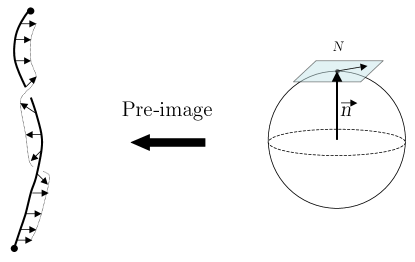
Figure 6: The pre-image of the North pole in the $S^{2}$ target space of $\vec{n}$ is a collection of arcs connecting hedgehogs. A fixed tangent vector at the North pole defines a vector field along the arcs, thereby making them framed arcs, which may be viewed as ribbons.

Now consider defects in the $\vec{n}$ field, which are classified by ${\pi_{2}}({S^{2}})=\mathbb{Z}$. Defects with winding number $\pm 1$ are positive and negative hedgehogs. For simplicity, we will focus on these; higher winding number hedgehods can be built up from these. (In the real model, as opposed to the toy model, the ‘hedgehogs’ have a $\mathbb{Z}_{2}$ classification so there are no higher winding number hedgehogs and, in fact, they do not even have a sign.) As noted by Teo and Kane Teo10, the $\vec{n}$ field around a hedgehog can be visualized in a simplified way, following Wilczek and Zee’s discussion of the Hopf term in a $2+1$-D O(3) non-linear $\sigma$ modelWilczek83. The field $\vec{n}$ can be viewed as a map from the physical space where the electrons live, $\mathbb{R}^{3}$. If we assume that the total winding number is zero (equal numbers of + and - hedgehogs) and that $\vec{n}$ approaches a constant at $\infty$, we can compactify the physical space $\mathbb{R}^{3}$ so that it is $S^{3}$. The target space of the map is $S^{2}$. The pre-image of the north pole $N\in S^{2}$ is a set of arcs and loops. The choice of the north pole $N$ is arbitrary, and any other point on the sphere would be just as good for the following discussion. Let’s ignore the loops for the moment and focus on the arcs. Since $\vec{n}$ points in every direction at a hedgehog, the arcs terminate at hedgehogs. In fact, each arc connects a $+1$ hedgehog to a $-1$ hedgehog. We now pick an arbitrary unit vector in the tangent space of the sphere at $N$. This vector can be pulled back to $S^{3}$ to define a vector field along the arcs which is clearly normal to the arcs. This is a framing, which allows us to define, for instance, a self-winding number for an arc. Intuitively, we can think of a framing as a thickening of an arc into a ribbon. Thus, the field $\vec{n}$ allows us to to define a set of framed arcs connecting the hedgehogs – in other words, a set of ribbons connecting the hedgehogs. As the normal vector twists around an arc, the ribbon twists, as shown in Fig. 6 (Although we will draw the ribbons as bands in the physical space, their width should not be taken seriously; they should really be viewed as arcs with a normal vector field.)

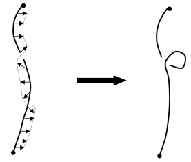
Figure 7: We will depict framed arcs or ribbons as arcs with twists accounted for by drawing kinks in the arcs, as shown above.

Although these ribbons are strongly reminiscent of particle trajectories, it is important to keep in mind that they are not. A collection of ribbons connecting hedgehogs defines a state of the system at an instant of time. Ribbons, unlike particle trajectories, can cross. They can break and reconnect as the system evolves in time. As hedgehogs are moved, the ribbons move with them.

A configuration of particles connected pairwise by ribbons is a seemingly crude approximation to the full texture defined by $\vec{n}$. However, according to the Pontryagin-Thom construction, as we describe in the next Section (and explain in Appendix LABEL:sec:appendix_pontryagin_thom_construction), it is just as good as the full texture for topological purposes. Thus, we focus on the space of particles connected pairwise by ribbons.

We now consider a collection of such particles and ribbons. For a topological discussion, all that we are interested in about the ribbons is how many times they twist, so we will not draw the framing vector but will, instead, be careful to put kinks into the arcs in order to keep track of twists in the ribbon, as depicted in Fig. 7. The fundamental group of their configuration space is the set of transformation which return the particles and ribbons to their initial configurations, with two such transformations identified if they can be continuously deformed into each other. Consider an exchange of two $+1$ hedgehogs, as depicted in Fig. 8. Although this brings the particles back to their initial positions (up to a permutation, which is equivalent to their initial configuration since the particles are identical), it does not bring the ribbons back to their initial configuration. Therefore, we need to do a further motion of the ribbons. By cutting and rejoining them as shown in Fig. 9a, a procedure which we call ‘recoupling’, we now have the ribbons connecting the same particles as in the initial configuration. But the ribbon on the left has a twist in it. So we rotate that particle by $-2\pi$ in order to undo the twist, as in Fig. 9b.

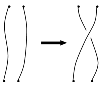
Figure 8: When two defects are exchanged, the $\vec{n}$-field around them is modified. This is encapsulated by the dragging of the framed arcs as the defects are moved.

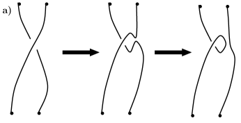
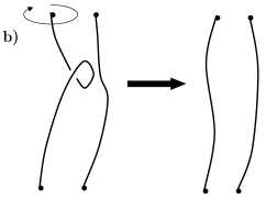
Figure 9: (a) In order to restore the framed arcs so that they are connecting the same defects, it is necessary to perform a recoupling by which they are reconnected. In order to keep track of the induced twist, it is easiest to perform the recoupling away from the overcrossing. (b) The particle on the left must be rotated by $-2\pi$ in order to undo a twist in the framed arc to which it is attached.

Let us use $t_{i}$ to denote such a transformation, defined by the sequence in Figs. 8, 9a, and 9b. The $t_{i}$s do not satisfy the multiplication rules of the permutation group. In particular, ${t_{i}}\neq t_{i}^{-1}$. The two transformations ${t_{i}}$ and $t_{i}^{-1}$ are not distinguished by whether the exchange is clockwise or counter-clockwise – this is immaterial since a clockwise exchange can be deformed into counter-clockwise one – but rather by which ribbon is left with a twist which must be undone by rotating one of the particles.

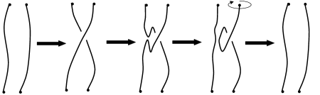
Figure 10: The sequence of moves which defines $t_{i}^{-1}$. (Here, the $i^{\rm th}$ particle is at the top left and the $(i+1)^{\rm th}$ is at the top right.) This may be contrasted with the sequence in Figs. 8, 9a, and 9b, which defines ${\sigma_{i}^{1}}$.

To see that the operations $t_{i}$, defined by the sequence in Figs. 8, 9a, and 9b, and $t_{i}^{-1}$, defined by the sequence in 10, are, in fact, inverses, it is useful to note that when they are performed sequentially, they involve two $2\pi$ twists of the same hedgehog. In 9b, it is the hedgehog on the left which is twisted; this hedgehog moves to the right in the first step of 10 and is twisted again in the fourth step. One should then note that a double twist in a ribbon can be undone continuously by using the ribbon to “lasso” the defect, a famous fact related to the existence of spin-$1/2$ and the fact that ${\pi_{1}}(SO(3))=\mathbb{Z}_{2}$. This is depicted in Fig. LABEL:fig:lassomove in Appendix LABEL:sec:Postnikov. It will be helpful for our late discussion to keep in mind that $t_{i}$ not only permutes a pair of particles but also rotates one of them; any transformation built up by multiplying $t_{i}$s will enact as many $2\pi$ twists as pairwise permutations modulo two.

Thus far we have only discussed the $+1$ hedgehogs. We can perform the similar transformations which exchange $-1$ hedgehogs. We will not repeat the above discussion for $-1$ hedgehogs since the discussion would be so similar; furthermore, in the $N\rightarrow\infty$ model which is our main interest, defects do not carry a sign, so they can all be permuted with each other.

We have concluded that ${t_{i}}\neq t_{i}^{-1}$ and, therefore, the group of transformations which bring the hedgehogs and ribbons back to their initial configuration is not the permutation group. This leaves open the question: what is ${t_{i}}^{2}$? The answer is that $t_{i}^{2}$ can be continuously deformed into a transformation which doesn’t involve moving any of the particles – Teo and Kane’s ‘braidless operations’. Consider the transformation $x_{i}$ depicted in Fig. 11. Defect $i$ is rotated by $2\pi$, the twist is transferred from one ribbon to the other, and defect $i+1$ is rotated by $-2\pi$. Since a $4\pi$ rotation can be unwound, as depicted in Fig. LABEL:fig:lassomove, ${x_{i}^{2}=1}$.

Intuitively, one expects that ${x_{i}}={t_{i}}^{2}$ since neither ${x_{i}}$ nor ${t_{i}}^{2}$ permutes the particles and both of them involve $2\pi$ rotations of both particles $i$ and $i+1$. To show that this is, in fact, the correct, we need to show that the history in Fig. 11 can be deformed into the sequence of Figs. 8, 9a, 9b repeated twice. If the history in Fig. 11 is viewed as a ‘movie’ and the sequence of Figs. 8, 9a, 9b repeated twice is viewed as another ‘movie’, then we need a one-parameter family of movies – or a ‘movie of movies’ – which connects the two movies. We will give an example of such a ‘movie of movies’ shortly. With this example in hand, the reader can verify that ${x_{i}}={t_{i}}^{2}$ by drawing the corresponding pictures, but we will not do so here since this discussion is superseded, in any case, by the the next section, where a similar result is shown for the $N\rightarrow\infty$ problem by more general methods. We simply accept this identity for now.

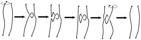
Figure 11: The sequence of moves which defines $x_{i}$: the defect on the left is rotated by $2\pi$, the twist is transfered to the ribbon on the right by two recouplings, and then the defect on the right is rotated by $-2\pi$. (Here, the $i^{\rm th}$ defect is at the top left and the $(i+1)^{\rm th}$ is at the top right.) The defects themselves are not moved in such a process.

We now consider the commutation relation for the $x_{i}$s. Clearly, for $|i-j|\geq 2$, ${x_{i}}{x_{j}}={x_{j}}{x_{i}}$. It is also intuitive to conclude that

$${x_{i}}x_{i+1}=x_{i+1}{x_{i}}$$ (61)

since the order in which twists are transferred is seemingly unimportant. However, since this is a crucial point, we verify it by showing in Figure 12 that the sequence of moves which defines ${x_{i}}x_{i+1}$ (a ‘movie’) can be continuously deformed into the sequence of moves which defines $x_{i+1}{x_{i}}$ (another ‘movie’). Such a deformation is a ‘movie of movies’; going from left-to-right in Fig. 12 corresponds to going forward in time while going from up to down corresponds to deforming from one movie to another.

Figure 12: The sequence of moves which defines ${x_{i}}x_{i+1}$ is shown in the top row. The sequence of moves which defines $x_{i+1}{x_{i}}$ is shown in the bottom row. The rows in between show how the top row can be continuously deformed into the bottom one. Such a deformation of two different sequences is a ‘movie of movies’ or a two-parameter family of configurations. Moving to the right increases the time parameter while moving down increases the deformation parameter which interpolates between ${x_{i}}x_{i+1}$ and $x_{i+1}{x_{i}}$.

Thus, we see that the equivalence class of motions of the defects (i.e. $\pi_{1}$ of their configuration space) has an Abelian subgroup generated by the $x_{i}$s. Since ${x_{i}^{2}}=1$ and they all commute with each other, this is simply $n-1$ copies of $\mathbb{Z}_{2}$, or, simply, $(\mathbb{Z}_{2})^{n-1}$.

In order to fully determine the group of transformations which bring the hedgehogs and ribbons back to their initial configuration, we need to check that the $t_{i}$s generate the full set of such transformations – i.e. that the transformations described above and those obtained by combining them exhaust the full set. In order to do this, we need the commutation relations of the $t_{i}$s with each other. Clearly, ${t_{i}}{t_{j}}={t_{j}}{t_{i}}$ for $|i-j|\geq 2$ since distant operations which do not involve the same hedgehogs nor the same ribbons must commute. On the other hand operations involving the same hedgehogs or ribbons might not commute. For instance,

$${t_{i}}x_{i+1}=x_{i}x_{i+1}t_{i}$$ (62)

To see why this is true, note that if we perform $x_{i+1}$ first, then defects $i+1$ and $i+2$ are twisted by $2\pi$. However, $t_{i}$ then permutes $i$ and $i+1$ and twists $i$ by $2\pi$. Thus, the left-hand-side permutes $i$ and $i+1$ and only twists $i+2$. The $(i+1)^{\rm th}$ hedgehog was twisted by $x_{i+1}$ and then permuted by $t_{i}$ so that it ended up in the $i^{\rm th}$ position, where it was twisted again in the last step in $t_{i}$; two twists can be continuously deformed to zero, so this hedgehog is not twisted at all. The right-hand-side similarly permutes $i$ and $i+1$ and only twists $i+2$ by $2\pi$. The reader may find it instructive to flesh out the above reasoning by constructing a movie of movies.

The multiplication rule which we have just described (but not fully justified) is that of a semi-direct product, which is completely natural in this context: when followed by a permutation, a transfer of twists ends up acting on the permuted defects. The twists $x_{i}$ form the group $(\mathbb{Z}_{2})^{n-1}$ which we can represent by $n$-component vectors all of whose entries are $0$ or $1$ which satisfy the constraint that the sum of the entries is even. The entries tell us whether a given hedgehog is twisted by $2\pi$ or not. In any product of $x_{i}$s, an even number of hedgehogs is twisted by $2\pi$. Now consider, for $n$ odd, the group elements given by

$${\sigma_{i}}=x_{n-1}x_{n-3}\ldots x_{i+3}x_{i+1}x_{i-2}x_{i-4}\ldots x_{1}\,t_{i}$$ (63)

for $i$ odd and

$${\sigma_{i}}=x_{n-1}x_{n-3}\ldots x_{i+2}x_{i}x_{i-1}x_{i-3}\ldots x_{1}\,t_{i}$$ (64)

for $i$ even. From (62), we see that ${{\sigma_{i}}^{2}}=1$. The group element $\sigma_{i}$ permutes the $i^{\rm th}$ and $(i+1)^{\rm th}$ hedgehogs and twists all of the hedgehogs. Thus, the $\sigma_{i}$s generate a copy of the permutation group $S_{n}$. The $\sigma_{i}$s do not commute with the $x_{i}$s, however; instead they act according to the semi-direct product structure noted above. On the other hand, the situation is a bit different for $n$ even. This may be a surprise since one might expect that $n$ even is the same as $n$ odd but with the last hedgehog held fixed far away. While this is true, exchanging the last hedgehog with the others brings in an additional layer of complexity which is not present for $n$ odd. The construction above, Eqs. 63, 64, does not work. One of the hedgehogs will be left untwisted by such a construction; since subsequent $\sigma_{i}$s will permute this untwisted hedgehog with others, we must keep track of the untwisted hedgehog and, therefore, the $\sigma_{i}$s will not generate the permutation group. In the even hedgehog number case, the group of tranformations has a $(\mathbb{Z}_{2})^{n-1}$ subgroup, as in the odd case, but there isn’t an $S_{n}$ subgroup, unlike in the odd case. To understand the even case, it is useful to note that in both cases, every transformation either (a) twists an even number of ribbons, which is the subgroup $(\mathbb{Z}_{2})^{n-1}$; (b) performs an even permutation, which is the subgroup $A_{n}$ of $S_{n}$; or (c) twists an odd number of ribbons and performs an odd permutation. Another way of saying this is that the group of transformations is the ‘even part’ of $(\mathbb{Z}_{2})^{n}\rtimes S_{n}$: the subgroup of $(\mathbb{Z}_{2})^{n}\rtimes S_{n}$ consisting of those elements whose $(\mathbb{Z}_{2})^{n}$ parity added to their $S_{n}$ parity is even. In the odd hedgehog number case, this is the semidirect product $(\mathbb{Z}_{2})^{n-1}\rtimes S_{n}$; in the even hedgehog number case, it is not. As we will see in Section LABEL:sec:projective, the difference between the even and odd hedgehog number cases is related to the fact that, for an even number of hedgehogs, the Hilbert space decomposes into even and odd total fermion number parity sectors. By contrast, the situation is simpler for an odd number of hedgehogs, where the parity of the total fermion number is not well-defined and the representation is irreducible.

To summarize, we have given some plausible heuristic arguments that the ‘statistics’ of $+1$ hedgehogs in a model of $2N=8$ Majorana fermions is governed by a group $E((\mathbb{Z}_{2})^{n}\rtimes S_{n})$, the ‘even part’ of $(\mathbb{Z}_{2})^{n}\rtimes S_{n}$: those elements of $(\mathbb{Z}_{2})^{n}\rtimes S_{n}$ in which the parity of the sum of the entries of the element in $(\mathbb{Z}_{2})^{n}$ added to the parity of the permutation in $S_{n}$ is even. (The same group governs the $-1$ hedgehogs). Rather than devoting more time here to precisely determining the group for the toy model, we will move on to the problem which is our main concern here, a system of $2N\rightarrow\infty$ Majorana fermions. This problem is similar, with some important differences. (1) The target space is no longer $S^{2}$ but is, instead, $U(N)/O(N)$. (2) Consequently, the defects do not carry a sign. There is no preferred pairing into $\pm$ pairs; the defects are all on equal footing. All $2n$ of them can be exchanged. (3) The group obtained by computing $\pi_{1}$ of the space of configurations of $2n$ defects then becomes the direct product of the ‘ribbon permutation group’ ${\cal T}^{r}_{2n}$ with a trivial ${\mathbb{Z}}$, ${\cal T}_{2n}={\mathbb{Z}}\times{\cal T}^{r}_{2n}$. The ribbon permutation group ${\cal T}^{r}_{2n}$ is given by ${\cal T}^{r}_{2n}\equiv{\mathbb{Z}}_{2}\times E((\mathbb{Z}_{2})^{2n}\rtimes S_{2n})$, where $E((\mathbb{Z}_{2})^{2n}\rtimes S_{2n})$ is the ‘even part’ of $(\mathbb{Z}_{2})^{2n}\rtimes S_{2n}$.

V Fundamental Group of the Multi-Defect Configuration Space

In Section III we concluded that the effective target space for the order parameter of a system of fermions in 3D with no symmetries is $U(N)/O(N)$ – which, as is conventional, we will simply call $U/O$, dropping the $N$ in the large-$N$ limit. This enables us to rigorously define the space of topological configurations, $K_{2n}$, of $2n$ hedgehogs in a ball, and calculate its fundamental group $\pi_{1}(K_{2n})$, thereby elucidating Teo and Kane’s Teo10 hedgehog motions and unitary transformations.

We now outline the steps involved in this calculation:

• We approximate the space $U/O$ by a cell complex (or CW complex), ${\cal C}$, a topological space constructed by taking the union of disks of different dimensions and specifying how the boundary of each higher-dimensional disk is identified with a subset of the lower-dimensional disks. This is a rather crude approximation in some respects, but it is sufficient for a homotopy computation.

• We divide the problem into (a) the motion of the hedgehogs and (b) the resulting deformation of the field configuration between the hedgehogs. This is accomplished by expressing the configuration space in the following way. Let us call the configuration space of $2n$ distinct points in three dimensions $X_{2n}$. (For the sake of mathematical convenience, we will take our physical system to be a ball $B^{3}$ and stipulate that the points must lie inside a ball $B^{3}$. Let’s denote the space of field configurations by ${\cal M}_{2n}$. This space is the space of maps to $U/O$ from $B^{3}$ with $2n$ points (at some standard locations) excised. The latter space is denoted by ${B^{3}}\,\backslash\,2n\mbox{ standard points}$. Since we will be approximating $U/O$ by ${\cal C}$, we can take ${\cal M}_{2n}$ to be the space of maps from ${B^{3}}\,\backslash\,2n\mbox{ standard points}$ to ${\cal C}$ with boundary conditions at the $2n$ points specified below. Then, there is a fibration of spaces:

  $$\!ifnextchar[{\beginpicture\setcoordinatesystem units<1pt,1pt>{0}}{\beginpicture\setcoordinatesystem units<1pt,1pt>}\!ifnextchar[{\!ifnextchar[{{2}{a}{\mathcal{M}_{2n}}}{{2}}}$$