The sub-arcsecond hard X-ray structure of loop footpoints in a solar flare

Abstract

The newly developed X-ray visibility forward fitting technique is applied to Reuven Ramaty High Energy Solar Spectroscopic Imager (RHESSI) data of a limb flare to investigate the energy and height dependence on sizes, shapes, and position of hard X-ray chromospheric footpoint sources. This provides information about the electron transport and chromospheric density structure. The spatial distribution of two footpoint X-ray sources is analyzed using PIXON, Maximum Entropy Method, CLEAN and visibility forward fit algorithms at nonthermal energies from $\sim 20$ to $\sim 200$ keV. We report, for the first time, the vertical extents and widths of hard X-ray chromospheric sources measured as a function of energy for a limb event. Our observations suggest that both the vertical and horizontal sizes of footpoints are decreasing with energy. Higher energy emission originates progressively deeper in the chromosphere consistent with downward flare accelerated streaming electrons. The ellipticity of the footpoints grows with energy from $\sim 0.5$ at $\sim 20$ keV to $\sim 0.9$ at $\sim 150$ keV. The positions of X-ray emission are in agreement with an exponential density profile of scale height $\sim 150$ km. The characteristic size of the hard X-ray footpoint source along the limb is decreasing with energy suggesting a converging magnetic field in the footpoint. The vertical sizes of X-ray sources are inconsistent with simple collisional transport in a single density scale height but can be explained using a multi-threaded density structure in the chromosphere.

1. Introduction

In the standard flare scenario, electrons that were accelerated in the corona stream downwards toward the dense layers of the solar atmosphere, where they are stopped via collisions producing intense hard X-ray (HXR) emission in the chromosphere. Higher energy electrons penetrate deeper into the chromosphere. Therefore, measurements of the spatial structure of the HXR emission as a function of energy provide information about the chromospheric density. Being optically thin, X-rays give the most direct information about the spatial and energy distribution of energetic electrons in the solar atmosphere. Prior to the launch of the Ramaty High Energy Solar Spectroscopic Imager (RHESSI) (Lin et al., 2002), HXR instruments typically had limited imaging-spectroscopy capabilities (Kosugi et al., 1992). RHESSI’s aptitude to image in various energy ranges opens new horizons for studying the detailed structure of HXR emitting sources in the chromosphere.

RHESSI does not directly image the Sun but uses 9 pairs of Rotating Modulation Collimators (RMCs) to time-modulate spatial information in the signal obtained in its germanium detectors (Hurford et al., 2002). Each RMC has a different thickness of its slits and slats making it sensitive to different spatial scales, providing modulation at nine spatial frequencies. The reconstruction of an image from these time modulated lightcurves, can be accomplished by various imaging algorithms Emslie et al. (2003); Battaglia & Benz (2007); Krucker & Lin (2008); Saint-Hilaire et al. (2008); Dennis & Pernak (2009). The new visibility based approach to RHESSI imaging starts by summing (stacking) the lightcurves per roll bins over a few spin periods of the spacecraft (Schmahl et al., 2007). The fitted amplitudes and the phases in the individual roll bins are X-ray visibilities. This effectively provides two dimensional spatial Fourier components (X-ray visibilities) over a wide range of energies (Hurford et al., 2002; Schmahl et al., 2007). To convert the time-modulated signal or X-ray visibilities to an image is an inverse problem (e.g. Piana et al., 2007; Prato et al., 2009). The reconstructed images face unavoidable difficulties due to measurement errors, finite coverage in Fourier space, and ill-posedness of the reconstruction problem. The resulting reconstruction errors and small dynamic range makes it difficult to accurately measure source sizes from reconstructed images. At best the imaging resolution is down to 2 arcseconds but in practice is around 7 arcseconds for the typical flare nonthermal energy range.

However, the moments of X-ray source distribution (source position, source size, etc) can be inferred with higher precision either from the time-modulated signal Aschwanden et al. (2002); Krucker & Lin (2008); Saint-Hilaire et al. (2008); Fivian et al. (2009) or visibilities (Xu et al., 2008; Kontar et al., 2008; Dennis & Pernak, 2009; Prato et al., 2009). Thus, RHESSI measurements of X-ray source positions can recover sub-arcsecond information using RHESSI modulated lightcurves (Aschwanden et al., 2002; Liu et al., 2006; Mrozek, 2006) or visibilities (Kontar et al., 2008; Dennis & Pernak, 2009; Prato et al., 2009). This has allowed clear demonstration of the height-energy dependence of HXR sources: higher energy sources originate at lower heights (Aschwanden et al., 2002; Brown et al., 2002; Liu et al., 2006). This has substantially improved upon previous results with Yohkoh/HXT (Matsushita et al., 1992). The recently developed visibility-based technique (Schmahl et al., 2007), allowed Kontar et al. (2008) to improve previous measurements and infer characteristic sizes (FWHM) of HXR footpoints and not just the centroid height. From this the convergence of the magnetic flux and neutral hydrogen density distribution in the chromosphere was inferred.

In this paper we study the structure of solar flare hard X-ray sources using various imaging algorithms: PIXON, MEM, CLEAN and visibility forward fit. Using RHESSI X-ray visibilities we find the characteristic shapes and positions for different energy ranges. We show that the technique of forward fitting X-ray visibilities allows us to determine not only the FWHM of the sources but vertical and horizontal sizes of the sources, which is required for examining the density structures of the chromosphere. Theoretical relationships were compared with observations to find the density structure of the chromosphere. The vertical size of the X-ray sources is found to be larger than the ones predicted by a hydrostatic atmosphere in thick-target scenario. However, assuming that the electrons are propagating along several narrow threads with different density profiles can explain the measured vertical sizes of the sources.

2. X-ray visibilities and characteristic sizes

The spatial information about an X-ray source measured by RHESSI for a given energy range and time interval can be presented (Hurford et al., 2002; Schmahl et al., 2007) as two dimensional Fourier components or X-ray visibilities

$$V(u,v;\epsilon)=\int_{x}\int_{y}I(x,y;\epsilon)e^{2\pi i(xu+yv)}dxdy$$ (1)

where $I(x,y;\epsilon)$ is the observed image at photon energy $\epsilon$. Then, reconstructed X-ray image $I(x,y;\epsilon)$ is the inverse Fourier transformation of measured X-ray visibilities $V(u,v;\epsilon)$. Each of the nine RHESSI Rotating Modulating Collimators (RMC) measures $V(u,v;\epsilon)$ at a fixed spatial frequency (or a circle in the $(u,v)$ plane) corresponding to its angular resolution and with a position angle along the circles, which varies continuously as the spacecraft rotates. Nine detector grids with angular resolutions growing with detector number are logarithmically spaced in the $(u,v)$ plane. Since the measured visibilities sparsely populate the $(u,v)$ plane and have statistical uncertainties, the direct inverse Fourier transform is impractical (Hurford et al., 2002; Schmahl et al., 2007; Massone et al., 2009) and alternative methods should be used.

Assuming a characteristic shape of X-ray source, one can find the position and characteristic sizes directly by fitting a 2D Fourier image of the model to the RHESSI visibilities. Here, we assume that the sources can be presented as elliptical Gaussian sources

$$I(x,y;\epsilon)=\frac{I_{0}(\epsilon)}{2\pi\sigma_{x}\sigma_{y}}\exp\left(-\frac{(x-x_{0}(\epsilon))^{2}}{2\sigma_{x}^{2}}-\frac{(y-y_{0}(\epsilon))^{2}}{2\sigma_{y}^{2}}\right),$$ (2)

where $2\sqrt{2\ln 2}\sigma_{x}$ and $2\sqrt{2\ln 2}\sigma_{y}$ are FWHMs of an elliptical Gaussian source in $x$ and $y$ direction respectively, $x_{0}(\epsilon)$, $y_{0}(\epsilon)$ is the position of the source, and $I_{0}$ is the total photon flux of the source. One major advantage of the visibility forward fit approach is that knowing the errors on visibilities $V(u,v;\epsilon)$ one can readily propagate the errors to forward fit parameters of the model in Equation (2). Reliable error estimates for images reconstructed with other algorithms are currently unavailable.

2.1. The shape of footpoints for a limb event

Using HXR data from RHESSI we analysed a limb event on January 6th, 2004 (GOES M5.8 class). As shown previously by (Kontar et al., 2008), this event is ideally suited for our analysis having two well separated footpoints: one bright and a second much weaker footpoint. In addition, the location of the flare at the limb greatly reduces albedo flux (Bai & Ramaty, 1978; Kontar & Jeffrey, 2010), so that the albedo correction (Kontar et al., 2006) becomes negligible.

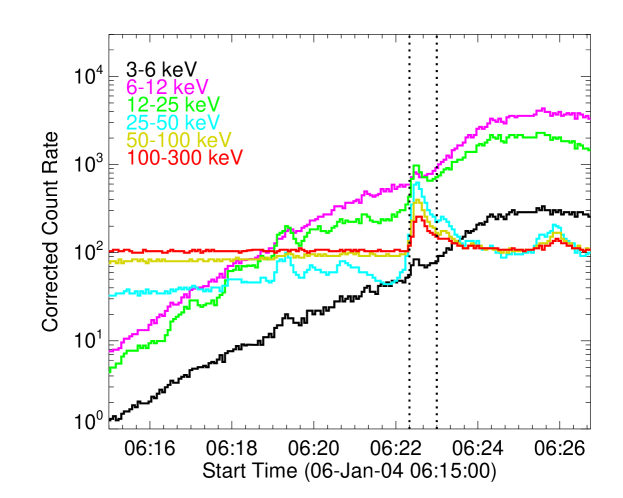
Figure 1.— Lightcurves of the 6-Jan-2004 flare. The vertical dotted lines show the accumulation time interval 06:22:20-06:23:00 UT which is used in the subsequent spectral and imaging analysis.

The flare occurred at the eastern limb near $(-975,75)$ arcseconds from the disk center at $\sim 06:22$ UT (Figure 1). It was imaged during the time of peak emission $>50$ keV 06:22:20-06:23:00 UT indicated by the vertical dotted lines in Figure 1, using four different image algorithms (see Figure 2): Clean (Hurford et al., 2002), MEM NJIT (Schmahl et al., 2007), PIXON (Pina & Puetter, 1993; Metcalf et al., 1996) and visibility forward fit (Hurford et al., 2002; Schmahl et al., 2007). The resulting images in five energy bands covering the nonthermal emission are shown in Figure 2. Each image was made using the front segments of detectors 2 to 7. Grid 1 with the highest spatial resolution had no significant signal and grids 8-9 are too coarse for our flaring region. Previously the flare was imaged using ten energy bins (Kontar et al., 2008) and simple circular gaussian fit but this was reduced to five wider bins in this paper to improve signal to noise. Figures 2,3 demonstrate that the brighter source has an elliptical shape at various energies, so an elliptical Gaussian could be used as natural X-ray distribution model (Figure 3).

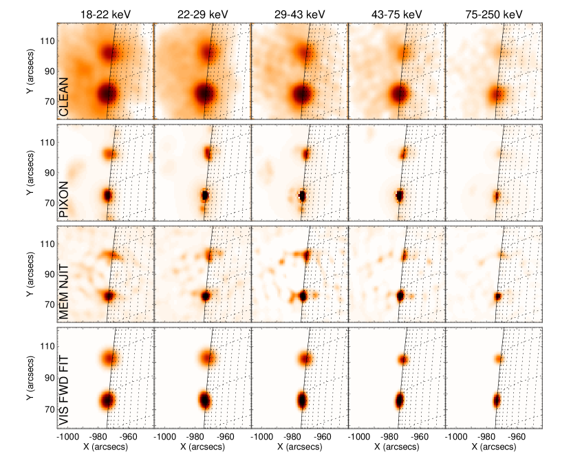
Figure 2.— HXR images of the January 6th 2004 flare (accumulation time interval 06:22:20-06:23:00 UT) in 5 energy ranges: 18-25, 25-29, 29-43, 43-75, 75-250 keV (energy grows from left to right) using different algorithms: (from top row to bottom) CLEAN, PIXON, MEM-NJIT, VIS forward fit. Image sizes are $64\times 64$ with a pixel size of $1\times 1$ arcseconds. Visibility forward fit images shown here were done using one elliptical (strong southern footpoint) and circular (weak northern footpoint) Gaussian.

Comparing the different algorithm results we find that CLEANed images have systematically larger sizes than the other algorithms. This is related to the fact that CLEAN images are determined by the user choices for analysis (clean beam size) and not the requirements of the data and hence should be used with great care to measure source sizes. MEM NJIT has produced smaller source sizes, which could be the tendency of the algorithm to over-resolve sources (Schmahl et al., 2007). PIXON (Pina & Puetter, 1993; Metcalf et al., 1995) gave source sizes similar to those of X-ray visibility forward fit. Dennis & Pernak (2009) have also analysed this event and confirmed the finding of Kontar et al. (2008). We choose to forward fit a circular Gaussian source for the northern footpoint and an elliptical Gaussian source (Equation 2) for the southern footpoint to the visibilities (Equation 1), the image shown is a reconstruction of the fit results. These fits are shown in Figure 3 and will be discussed in detail in §2.2. Assuming two elliptical sources, the weaker source forward fit parameters have rather large error bars suggesting that Northern footpoint is not sufficiently well-constrained by the data to be fitted as an elliptical source. In addition, at the energies above $40$ keV the weak source is indistinguishable from circular.

The comparison of the images and visibility fit results in Figure 2 shows that visibility forward fit gives images similar to the ones inferred in other algorithms, although there are differences pointed out above. Despite the differences between the algorithms, all image reconstruction algorithms show that the southern footpoint has a) a clear elliptical shape, b) the shape of the source becomes more elliptical with growing energy c) the size of the source decreases with energy. The northern footpoint is also getting smaller with energy similar to the southern footpoint (Kontar et al., 2008; Dennis & Pernak, 2009), but due to lower count rate in the source we cannot reliably measure the shape of this source. In addition, since the northern source is not seen above $\sim 100$ keV, it could be partially occulted or have stronger magnetic convergence (Schmahl et al., 2006) with the energetic electrons precipitating less to dense layers of the chromosphere, producing a fainter footpoint.

2.2. Characteristic sizes and foot-point locations

We focus on the brighter southern footpoint fitted with an elliptical gaussian (Equation 2) as more spatial information can be accurately recovered compared to the northern footpoint. This is a more realistic interpretation of the footpoint shape (see Figure 2) compared to the previously used circular fit (Aschwanden et al., 2002; Kontar et al., 2008).

Each forward fit to X-ray visibilities using an elliptical gaussian produces 6 parameters given by Equation (2): positions $x_{0}(\epsilon)$ and $y_{0}(\epsilon)$ of the X-ray flux maximum (often called centroid position), full width half maximum $FWHM(\epsilon)$, eccentricity $e(\epsilon)$ and position angle $\theta(\epsilon)$, along with error values for each of the parameters. $x_{0}(\epsilon)$ and $y_{0}(\epsilon)$ are measured from disk centre and the position angle $\theta(\epsilon)$ is the angle between the North-South line and the semi-major axis of the ellipse. Multiple sources are fitted simultaneously and we fit the weaker northern source with a circular Gaussian. Both sources can be fitted with elliptical sources producing similar results for the southern footpoint but highly inaccurate results for the northern footpoint. The visibility amplitudes and fits as a function of RMC and spacecraft roll angle are shown in Figure 3. We used between 6 (course grids) and 12 (fine grids) visibilities (spatial Fourier components) (Figure 3). The single circular Gaussian fit shows the largest amplitudes of normalised residuals. Two circular Gaussian fit has smaller amplitudes, but larger than the fit using an elliptical and circular Gaussian fits. The circular plus elliptical fits adequately reproduce the measured photon flux for various roll bins and collimators. We note that at the lowest energies $18-22$ keV, both two circular and elliptical plus circular Gaussians give almost identical results. Indeed, both footpoints at $18-22$ keV look symmetrical (Figure 2). The largest deviations of the fits from the data is found in the coarsest grid and at the lowest energy (Figure 3), which could be caused by the large scale source ($\gtrsim 36^{\prime\prime}$), probably softer X-ray emission from the loop.

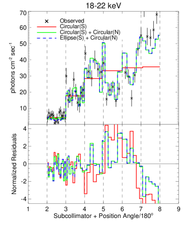
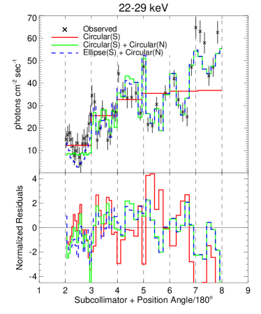
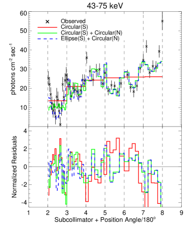
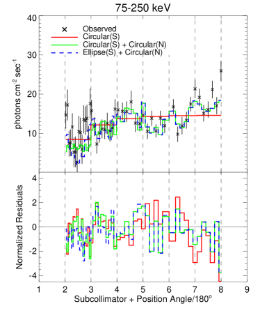
Figure 3.— Observed X-ray visibility amplitudes (crosses with error bars) as a function of subcollimator (2-7) and position angle between $0$ and $180^{o}$ of the grids in the stated energy range. The red line shows the fitted model using single circular source, the green line shows two circular Gaussian fits, and the blue dashed line shows an elliptical (southern footpoint) and circular (northern footpoint) Gaussian. The bottom panels show normalised residuals for the corresponding fits.

Using the $(x_{0}(\epsilon),y_{0}(\epsilon))$ “centroid positions” of the source for each energy range, the radial height of the source from the solar centre can be readily determined for every energy using:

$$R(\epsilon)=\sqrt[]{x_{0}(\epsilon)^{2}+y_{0}(\epsilon)^{2}}.$$ (3)

The semi-major and semi-minor axes of our elliptical gaussian fit, $a(\epsilon)$, $b(\epsilon)$ respectively are related to the FWHM:

$$\mbox{FWHM}(\epsilon)=\sqrt{a(\epsilon)b(\epsilon)},$$ (4)

and to the eccentricity by:

$$e(\epsilon)=\sqrt{1-b(\epsilon)^{2}/a(\epsilon)^{2}}.$$ (5)

Equations (4) and (5) can be solved to find

$$a(\epsilon)=FWHM(\epsilon)(1-e(\epsilon))^{-1/4},\quad b(\epsilon)=FWHM(\epsilon)(1-e(\epsilon))^{1/4}$$ (6)

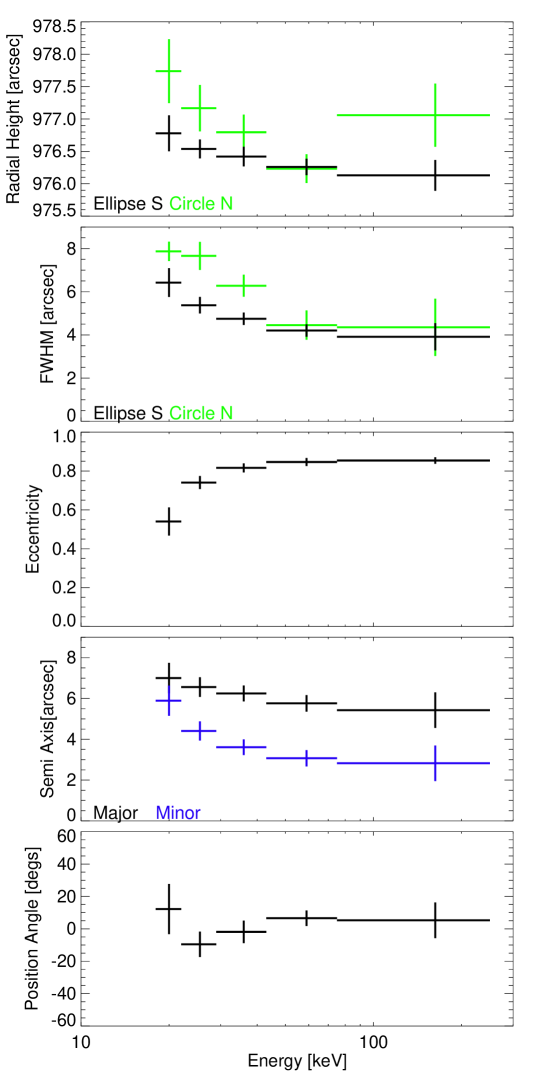
Figure 4.— X-ray visibilities forward fit parameters as a function of energy: radial distance of the sources, FWHM of the sources, eccentricity, semi-minor and semi-major axes for the northern footpoint, and position angle (the angle between semi-major axis and North-South direction).

As the analysed flare is right on the Eastern limb and close to the solar equator, $a(\epsilon)$ and $b(\epsilon)$ correspond to the source sizes parallel (width) and perpendicular (vertical extent) to the solar surface. The results of the X-ray visibility forward fit parameters are summarised in Figure 4. They again show the trend seen in the images (Figure 2) of decreasing height and source size with energy. We can also see that the source becomes more elliptical at higher energies, starting with $e\sim 0.5$ for 18-22 keV but increasing to $e\sim 0.85$ for 75-250 keV. The circular Gaussian source fitted to the northern footpoint also shows the general trend of decreasing source height and FWHM at higher energies but with considerably larger errors due to this source being weaker.

2.3. Height of X-ray sources above the photosphere

Let us consider the evolution of the electron flux spectrum in the chromosphere $F(E,s)$ along magnetic field lines $s$ using purely collisional transport and ignoring collective effects and effects connected with the magnetic mirroring (Brown et al., 2002). In this approximation the electron flux spectrum can be written (Brown, 1971)

$$F(E,s)=F_{0}(E_{0})\frac{E}{E_{0}}$$ (7)

where $F_{0}(E)$ is the injected spectrum of energetic electrons, taken to be a powerlaw of $F_{0}(E)\propto E^{-\delta}$ and

$$E_{0}(E,s)^{2}=E^{2}+2K\int_{0}^{s}n(s^{\prime})ds^{\prime}$$ (8)

where $K=2\pi e^{2}\ln\Lambda$, $\ln\Lambda$ is the Coulomb logarithm, $e$ is the electron charge. The chromosphere below the transition region can be conveniently assumed to be neutral (Brown, 1973; Kontar et al., 2002; Su et al., 2009) therefore $\ln\Lambda=\ln\Lambda_{eH}=7$ (e.g. Brown, 1973; Emslie, 1978).

The X-ray flux spectrum emitted by the energetic electrons in a magnetic flux tube of cross-sectional area $A$ and observed at 1AU is given as

$$I(\epsilon,s)=\frac{1}{4\pi R^{2}}An(s)\int_{\epsilon}^{\infty}F(E,s)\sigma(E,\epsilon)dE,$$ (9)

where $\sigma(E,\epsilon)$ is the isotropic bremsstrahlung cross-section, $R$ is the Sun-Earth distance, $A$ is the cross-sectional area of the loop. The X-ray flux spectrum expressed by Equation (9) has a maximum or equivalently $dI(\epsilon,s)/ds=0$ for every energy $\epsilon$ because of the growing density along electron path and simultaneously decreasing electron flux due to collisions (Brown et al., 2002; Aschwanden et al., 2002).

Assuming a hydrostatic density profile of

$$n(h=r-r_{0})=n_{0}\exp{\left(\frac{-(r-r_{0})}{h_{0}}\right)},$$ (10)

where $r$ is the radial distance from the Sun centre, the photospheric density $n_{0}=1.16\times 10^{17}$ cm^-3 [fixed value (Vernazza et al., 1981)], and $r_{0}$ is the reference height, we can find these two free parameters $h_{0}$ and $r=r_{0}$ by forward fitting the measured radial distance of maxima (Figure 5, bottom panel) to the model predicted maxima by the derivative of equation 9. The height of the sources can be found by subtracting the reference height, $\mathit{r_{0}}$, from the radial measurements:

$$h(\epsilon)=r(\epsilon)-r_{0}.$$ (11)

To calculate the reference height we assumed the density at the photospheric level to be known (Vernazza et al., 1981). This helps to remove substantial uncertainties related to the reference height of the previous studies (c.f. Aschwanden et al., 2002; Liu et al., 2006; Mrozek, 2006).

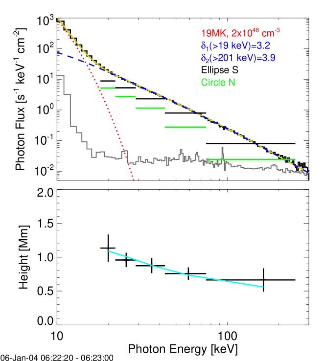
Figure 5.— Upper panel: X-ray spectrum of January 6, 2004 flare (solid black histogram) for the accumulation time 06:22:20-06:23:00 UT (see Figure 1) and forward fitted spectrum (yellow line). The photon spectrum was fitted using a thermal (red dotted line) plus thick-target model (blue dashed line). The gray histogram shows the background level. Horizontal black and green lines show the photon flux spectrum from the southern and northern footpoints as found in X-ray visibility forward fits (Figure 2) respectively. The lower panel indicate the results of the forward fit of the source height with collisional model. The fit results are $R_{0}=975.2^{\prime\prime}$, and $h_{0}=155$ km.

We find a spectral index of $\delta=3.2$ from the spatially integrated spectrum, shown in the top panel of Figure 5. Forward fitting using a hydrostatic density profile gives density scale height of $h_{0}=155\pm 30$ km and reference height $r_{0}=975.2\pm 0.2^{\prime\prime}$. From only fitting a circular gaussian to the southern footpoint, instead of elliptical to southern with circular to the northern as done in this paper, it was previously found that $h=140\pm 30$ km and $r_{0}=975.3\pm 0.2^{\prime\prime}$ (Kontar et al., 2008).

2.4. Vertical extent of the footpoint

The characteristic size of the source in the vertical direction (semi-minor axis in our fit) can be straightforwardly estimated using the collisional think-target model (Brown, 1971) to find the FWHM size from Equation 9 using the density profile found in the previous section. Comparing the measured vertical FWHM size and the prediction of the length from the thick-target model, we see that the measured extent is around $3-6^{\prime\prime}$ and is $3-6$ times larger than the theoretical width (Figure 6). The discrepancy is substantial and cannot be explained in terms of the assumed X-rays source model or error bars.

There are a few plausible explanations which can be given for the observed vertical FWHM size. One is that the structure of the chromosphere may not be uniform over the footpoint cross-section and the footpoint is the ensemble of many thin threads (Figure 7) as often seen in high resolution optical images (Lin et al., 2005; De Pontieu et al., 2007; Berkebile-Stoiser et al., 2009). Moreover, it is likely that the deposition of electron energy can lead to heating of the chromosphere upwards with the resulting expansion changing the density structure (e.g. Liu et al., 2009).

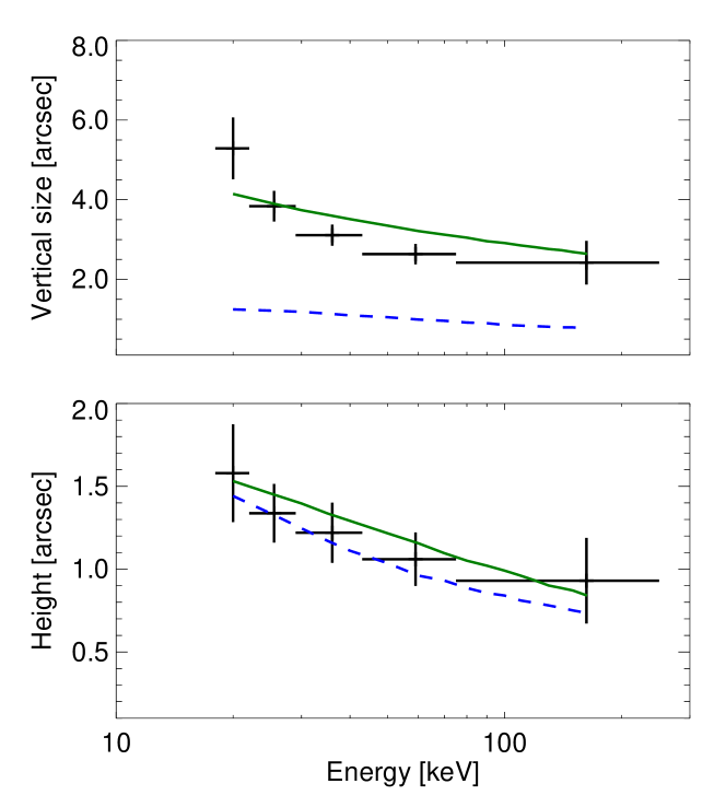
Figure 6.— Top panel: FWHM vertical size of the footpoint source (black crosses) as a function of energy; FWHM size given by the thick-target model (Equation 9) (blue dashed lines), multi-thread chromosphere (green lines). Bottom panel: height of the maximum X-ray emission (black crosses) versus energy.

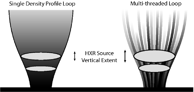
Figure 7.— Cross-sectionally uniform (left) and multi-threaded (right) chromospheres. The multi-thread chromosphere leads to the larger vertical sizes of X-ray sources as observed by RHESSI.

Let us consider a simple chromospheric model in which the hydrostatic density scale height, $h_{T}$, is determined by the temperature of the chromosphere $h_{T}=k_{b}T/(\mu m_{p}g)$ where $T$ is the temperature, $k_{b}$ is the Boltzman constant, $m_{p}$ is the proton mass, $\mu\simeq 1.27$ is the mean molecular weight (e.g. Aschwanden et al., 2002), and $g\simeq 2.74\times 10^{4}$ cm s^-2 is the solar gravitational acceleration. Thus, the measured density scale height of $\sim 155$ km implies an average chromospheric temperature of $\sim 6500$ K. However, the solar atmosphere is not a uniform media but instead is manifested in thin threads $(<0.3)^{\prime\prime}$ of filaments (Lin et al., 2005), sub-arcsecond dynamic fibrils (De Pontieu et al., 2007) and fine structure of microflares (Berkebile-Stoiser et al., 2009) in the chromosphere with different density profiles in each thread (Figure 7). Following the multi-thread model for the magnetic loop in the chromosphere, we assume that the energetic electrons propagate along different threads with varying density profiles and temperatures in the range from $2200$ K up to $20000$ K, corresponding to density scale heights between $\sim 50$ km and $\sim 500$ km. The average hard X-ray flux from many thin threads will be the measured X-ray distribution. Averaging X-ray emission from a hundred thin threads with temperatures drawn randomly from the above range, we successfully reproduce the observed vertical sizes (Figure 6).

3. Discussion and Conclusions

Using X-ray visibility forward fits, we inferred not only the characteristic sizes and positions but the shapes of HXR sources. The January 6th 2004 event indicates an overall decrease in size of the source and increase of the source ellipticity with energy. The FWHM of the southern source decreases from $\sim 6.5^{\prime\prime}$ down to around $\sim 4^{\prime\prime}$ while the ellipticity of the source grows from $0.5$ up to $0.9$. The source is elongated along the limb as evident in nearly zero angle between semi major-axis and the limb, such orientation of the source is observed for all energy ranges. The vertical extent of the source is decreasing by a larger fraction (from $6^{\prime\prime}$ down to $3^{\prime\prime}$) than the horizontal size (from $7^{\prime\prime}$ down to $5.5^{\prime\prime}$) leading to larger elongation of the source along the limb. Hence the FWHM of the magnetic flux tube containing energetic electrons (semi-major axis) changes from $\sim 9.7$ Mm at height $\sim 1.1$ Mm down to $\sim 7.6$ Mm at $0.6$ Mm above the photosphere. The northern footpoint is fainter, but shows a similar trend: the higher energies appear at low heights and the size of the source is decreasing with energy suggesting convergence of the magnetic field lines along which electrons propagate. Using X-ray visibilities we also re-analyzed a flare that occurred on February, 20th, 2002 that was previously studied by forward fitting time-modulated lightcurves (Aschwanden et al., 2002). Although this flare is rather weak, we found similar results: the higher energy sources appear at lower heights. The uncertainties are larger than in the January 6th, 2004 event but the density model proposed by Aschwanden et al. (2002) is within our error bars. We also note that the size of the sources in the February 20th flare decreases with energy similar to the event on January 6th.

Analysing HXR emission from footpoints we found that various imaging algorithms (PIXON, Visibility Forward Fit, CLEAN, MEM-NJIT) give generally similar results for spatial distributions of X-ray footpoints. Although RHESSI imaging algorithms can be adjusted by the parameter choice and hence X-ray images could be somewhat altered, there is a general trend for the algorithms. CLEAN with default set of parameters has a tendency to provide larger sources while MEM-NJIT tends to over-resolve X-ray sources. PIXON and visibility forward fit show very similar results. Visibility forward fit allows us to study sub-arcsecond distribution of hard X-ray sources in suitably orientated bright flares. Due to systematic differences in sizes we obtained for January 2004 and February, 2002 flares, we suggest that CLEAN and MEM-NJIT should be used for source size/shape measurements of X-ray sources with extreme caution.

The northern footpoint could be partially occulted as the highest energy photons come predominantly from the southern footpoint, but we note that this bright footpoint is unlikely to be occulted. As pointed out by G. Hurford, a source partially subtended by the solar disk should have a sharp edge, where the brightness of the source will drop from maximum to zero over rather small radial distance. The derivative of the source brightness in the $x$-direction (perpendicular to the limb), $\partial I(x,y)/\partial x$ will have a maximum at the limb, where $I(x,y)$ has a sharp drop. It is evident from Equation (1) that the corresponding visibilities, $2\pi iuV(u,v)$, should have a well pronounced maximum, which should be evident in the measured amplitudes of visibilities. Specifically, the finer grid RMCs should show large amplitudes when the grids are parallel to limb, i.e. the visibility amplitudes are much larger at the phase angles $~{}0^{o}$ and $~{}180^{o}$, which is not evident in the event under study (cf Figure 3). To make the discussion more complete, we note that the line of sight effects cannot be definitively ruled out. The footpoints might be projections of two rather long flare ribbons viewed almost parallel to the line of sight, so that the vertical extension is the projection of different height. Finally we should note that if the occultation height is small, $\lesssim 0.5^{\prime\prime}$, our height measurements are lower limits, but the major conclusion about the vertical extend is the same. If, though unlikely, the lower part of the loop (footpoints) is occulted, these observations provide an interesting question to the flare models as to why the sources sizes decrease with energy and the higher energy sources appear lower and not at the lowest visible location where the density is the highest.

Our measurements show that while the locations of the maxima of X-ray emission are consistent with simple collisional transport in single density scale height chromosphere, the vertical sizes do not agree with the assumption of field aligned electron transport. The vertical extent of X-ray sources is 3-6 times larger than in the purely collisional model in single-density-scale-height chromosphere. However, a chromospheric model involving multiple density threads within the flux tube of a footpoint can explain both the position of the maximum and the vertical size of the sources. We note that pitch angle scattering due to Coulomb collisions is likely to be insufficient to produce so strong expansion. The X-ray source size increase due to collisional pitch angle scattering will be about a quarter of the electron stoping depth for initially field aligned electrons (Conway, 2000). However, strong non-collisional scattering or wave-particle interactions (e.g. Hannah et al., 2009) might boost the vertical source sizes to the measured value and hence cannot be excluded and will also be consistent with lack of downward anisotropy found in X-ray flare emission (Kontar & Brown, 2006; Kašparová et al., 2007). We note that the adopted model does not account for the magnetic field and its effects on particle transport, which could lead to larger source sizes and is subject of additional modeling.

References

- Aschwanden et al. (2002) Aschwanden, M. J., Brown, J. C., & Kontar, E. P. 2002, Sol. Phys., 210, 383
- Bai & Ramaty (1978) Bai, T., & Ramaty, R. 1978, ApJ, 219, 705
- Battaglia & Benz (2007) Battaglia, M., & Benz, A. O. 2007, A&A, 466, 713
- Berkebile-Stoiser et al. (2009) Berkebile-Stoiser, S., Gömöry, P., Veronig, A. M., Rybák, J., & Sütterlin, P. 2009, A&A, 505, 811
- Brown (1971) Brown, J. C. 1971, Sol. Phys., 18, 489
- Brown (1973) —. 1973, Sol. Phys., 28, 151
- Brown et al. (2002) Brown, J. C., Aschwanden, M. J., & Kontar, E. P. 2002, Sol. Phys., 210, 373
- Conway (2000) Conway, A. J. 2000, A&A, 362, 383
- De Pontieu et al. (2007) De Pontieu, B., Hansteen, V. H., Rouppe van der Voort, L., van Noort, M., & Carlsson, M. 2007, ApJ, 655, 624
- Dennis & Pernak (2009) Dennis, B. R., & Pernak, R. L. 2009, ApJ, 698, 2131
- Emslie (1978) Emslie, A. G. 1978, ApJ, 224, 241
- Emslie et al. (2003) Emslie, A. G., Kontar, E. P., Krucker, S., & Lin, R. P. 2003, ApJ, 595, L107
- Fivian et al. (2009) Fivian, M. D., Krucker, S., & Lin, R. P. 2009, ApJ, 698, L6
- Hannah et al. (2009) Hannah, I. G., Kontar, E. P., & Sirenko, O. K. 2009, ApJ, 707, L45
- Hurford et al. (2002) Hurford, G. J., Schmahl, E. J., Schwartz, R. A., Conway, A. J., Aschwanden, M. J., Csillaghy, A., Dennis, B. R., Johns-Krull, C., Krucker, S., Lin, R. P., McTiernan, J., Metcalf, T. R., Sato, J., & Smith, D. M. 2002, Sol. Phys., 210, 61
- Kašparová et al. (2007) Kašparová, J., Kontar, E. P., & Brown, J. C. 2007, A&A, 466, 705
- Kontar & Brown (2006) Kontar, E. P., & Brown, J. C. 2006, ApJ, 653, L149
- Kontar et al. (2002) Kontar, E. P., Brown, J. C., & McArthur, G. K. 2002, Sol. Phys., 210, 419
- Kontar et al. (2008) Kontar, E. P., Hannah, I. G., & MacKinnon, A. L. 2008, A&A, 489, L57
- Kontar & Jeffrey (2010) Kontar, E. P., & Jeffrey, N. L. S. 2010, A&A, 513, L2+
- Kontar et al. (2006) Kontar, E. P., MacKinnon, A. L., Schwartz, R. A., & Brown, J. C. 2006, A&A, 446, 1157
- Kosugi et al. (1992) Kosugi, T., Sakao, T., Masuda, S., Makishima, K., Inda, M., Murakami, T., Ogawara, Y., Yaji, K., & Matsushita, K. 1992, PASJ, 44, L45
- Krucker & Lin (2008) Krucker, S., & Lin, R. P. 2008, ApJ, 673, 1181
- Lin et al. (2002) Lin, R. P., Dennis, B. R., Hurford, G. J., et al. 2002, Sol. Phys., 210, 3
- Lin et al. (2005) Lin, Y., Engvold, O., Rouppe van der Voort, L., Wiik, J. E., & Berger, T. E. 2005, Sol. Phys., 226, 239
- Liu et al. (2006) Liu, W., Liu, S., Jiang, Y. W., & Petrosian, V. 2006, ApJ, 649, 1124
- Liu et al. (2009) Liu, W., Petrosian, V., & Mariska, J. T. 2009, ApJ, 702, 1553
- Massone et al. (2009) Massone, A. M., Emslie, A. G., Hurford, G. J., Prato, M., Kontar, E. P., & Piana, M. 2009, ApJ, 703, 2004
- Matsushita et al. (1992) Matsushita, K., Masuda, S., Kosugi, T., Inda, M., & Yaji, K. 1992, PASJ, 44, L89
- Metcalf et al. (1996) Metcalf, T. R., Hudson, H. S., Kosugi, T., Puetter, R. C., & Pina, R. K. 1996, ApJ, 466, 585
- Metcalf et al. (1995) Metcalf, T. R., Jiao, L., McClymont, A. N., Canfield, R. C., & Uitenbroek, H. 1995, ApJ, 439, 474
- Mrozek (2006) Mrozek, T. 2006, Advances in Space Research, 38, 962
- Piana et al. (2007) Piana, M., Massone, A. M., Hurford, G. J., Prato, M., Emslie, A. G., Kontar, E. P., & Schwartz, R. A. 2007, ApJ, 665, 846
- Pina & Puetter (1993) Pina, R. K., & Puetter, R. C. 1993, PASP, 105, 630
- Prato et al. (2009) Prato, M., Emslie, A. G., Kontar, E. P., Massone, A. M., & Piana, M. 2009, ApJ, 706, 917
- Saint-Hilaire et al. (2008) Saint-Hilaire, P., Krucker, S., & Lin, R. P. 2008, Sol. Phys., 250, 53
- Schmahl et al. (2006) Schmahl, E. J., Pernak, R., & Hurford, G. 2006, in Bulletin of the American Astronomical Society, Vol. 38, Bulletin of the American Astronomical Society, 241–+
- Schmahl et al. (2007) Schmahl, E. J., Pernak, R. L., Hurford, G. J., Lee, J., & Bong, S. 2007, Sol. Phys., 240, 241
- Su et al. (2009) Su, Y., Holman, G. D., Dennis, B. R., Tolbert, A. K., & Schwartz, R. A. 2009, ApJ, 705, 1584
- Vernazza et al. (1981) Vernazza, J. E., Avrett, E. H., & Loeser, R. 1981, ApJS, 45, 635
- Xu et al. (2008) Xu, Y., Emslie, A. G., & Hurford, G. J. 2008, ApJ, 673, 576