An X-ray upper limit on the presence of a Neutron Star for the
Small Magellanic Cloud and Supernova Remnant 1E0102.2-7219
Abstract
We present Chandra X-ray Observatory archival observations of the supernova remnant 1E0102.2-7219, a young Oxygen-rich remnant in the Small Magellanic Cloud. Combining 28 ObsIDs for 324 ks of total exposure time, we present an ACIS image with an unprecedented signal-to-noise ratio (mean S/N 6; maximum S/N 35) . We search within the remnant, using the source detection software wavdetect, for point sources which may indicate a compact object. Despite finding numerous detections of high significance in both broad and narrow band images of the remnant, we are unable to satisfactorily distinguish whether these detections correspond to emission from a compact object. We also present upper limits to the luminosity of an obscured compact stellar object which were derived from an analysis of spectra extracted from the high signal-to-noise image. We are able to further constrain the characteristics of a potential neutron star for this remnant with the results of the analysis presented here, though we cannot confirm the existence of such an object for this remnant.
1 Introduction
The supernova remnant 1E 0102.2-7219 (SNR 1E0102.2-7219, hereafter,
“E0102”) was first identified by Seward & Mitchell, (1981) in a survey of the
Small Magellanic Cloud (SMC) with the Einstein X-Ray Observatory.
While this oxygen-rich remnant resides at a distance of 59 kpc
(van den Bergh, , 1999), it is far less extincted than many Galactic
remnants due to its high galactic latitude (l
–45∘). Kinematic studies in the X-ray and optical have
determined E0102 to be a relatively young remnant, with an expansion
age between 1000 and 2000 years (Hughes et al., , 2000; Finkelstein et al., , 2006, respectively).
For these reasons, E0102 has been extensively studied across the
electromagnetic spectrum radio (Amy & Ball, , 1993), IR
(Stanimirović et al., , 2005), optical (Tuohy & Dopita, , 1983; Blair et al., , 2000; Finkelstein et al., , 2006), UV (Blair et al., , 1989), and
X-ray (Hayashi et al., , 1994; Gaetz et al., , 2000; Rasmussen et al., , 2001; Flanagan et al., , 2004).
E0102 was likely generated by a Type Ib or Ic core-collapse supernova event (Blair et al., , 2000). As such, the remnant E0102 would be expected to host some variety of compact object (i.e., stellar mass black hole or degenerate stellar object). Furthermore, Amy & Ball, (1993) and Finkelstein et al., (2006) have considered the possibility that such a compact object may be influencing the complex morphology of this remnant. Though this remnant has been well studied, few groups have provided observational constraints to the presence of a compact object for E0102. In fact, only Gaetz et al., (2000) have presented an upper flux limit on a Crab-like pulsar for this remnant. In this research, we seek to constrain the X-ray luminosity of this unidentified compact object.
E0102 is a calibration target for the Chandra X-Ray Observatory facility team, and has been observed since Chandra’s 1999 launch. As a result, the Chandra Data Archive contains 2.16 million seconds of calibration observations acquired during 215 observing sessions (ObsIDs). Many of these observations were obtained to calibrate the off-axis performance of the detector. We use archive calibration data exclusively in this research, specifically those ObsIDs with high spatial resolution acquired on-axis between 2000 and 2009. With these combined data, we present new upper limits to the X-ray flux of a compact stellar object for the remnant.
2 Observations
We used Chandra archive calibration data of E0102 as observed with the Advanced CCD Imaging Spectrometer (ACIS; see Garmire et al., , 2003, for a review of ACIS). Of the more than 2 Ms of available Chandra calibration observations of E0102, we select those observations for which E0102 was imaged on the S3 chip in the ACIS-S configuration. We also require that the calibration imaging was obtained without spectral gratings in the beam. This selection criteria ensured that the remnant was not imaged across multiple chips, the optimal spatial resolution of 10 was achieved with on-axis pointings (see Chandra Proposers’ Observatory Guide, (2009) for more details), and also ensured a uniformity in the data set necessary for the spectral analysis presented in Section 4.2. The S3 chip is a back-illuminated CCD chip, and thus has higher sensitivity to lower energy photons than the front-illuminated I3 chip, making this chip the favorable one to use when characterizing any compact stellar object in the remnant with a soft spectral behavior (e.g. a Cas-A-like neutron star). The ObsIDs that met these criteria are listed in Table 1.
3 Data Reduction
Data reduction and processing were completed with the Chandra software package, CIAO version 4.1111see http://cxc.harvard.edu/ciao/, and IDL. The ObsIDs were processed with the CIAO routine acis_process_events to remove pixel randomization. For each ObsID, a lightcurve was generated for a background region beyond the remnant, to check for possible flaring events. Temporal variations above the mean background sky, which could indicate solar flaring events during the exposure, were found to be minimal, for each of the ObsIDs selected. A charge transfer inefficiency (CTI) correction was applied, to minimize the effects of radiation contamination which the Chandra detectors have experienced in orbit since launch. Next, the sub-pixel event re-positioning algorithm ser_v2, an IDL procedure, was applied to each exposure. This routine is designed to improve Chandra’s spatial resolution, by decomposing 2, 3, and 4 pixel photon splits at the chip interface (see Li et al., , 2003).
Using the CIAO script merge_all, the data were re-projected onto one common frame (ObsID 2843) and stacked to produce a single exposure with an effective exposure length of approximately 324 ks. The increase in the signal-to-noise for this combined image is a factor of 4 – 6 over the S/N of any individual ObsID. This stacked image is referred to as the merged image in the text. This, and all other, images which were used to complete the analysis we present here, at the native pixel scale of the ACIS detector 049 pixel-1.
4 Analysis
4.1 Image Analysis
4.1.1 Locating a Compact Stellar Object
Simulations and observations alike suggest that core-collapse supernova events are not likely to be spherically symmetric in their collapse (see Wang & Wheeler, , 2008, and references therein). It may be possible, or even requisite for some varieties of core-collapse supernovae, that this asymmetric evolution results in a “pre-natal kick” of the compact object revealed by the supernova event (Fryer et al., , 2006; Fragos et al., , 2009). We include this dynamic factor by defining an area in which a “kicked” stellar object would most likely be found. This “test source region” (hereafter, TSR) has a radius, r, estimated by , where is the “kick velocity” and is the expansion age of the remnant.
We use two published expansion ages to constrain for E0102. From the analysis of the X-ray proper motions of shell ejecta over a period of approximately 20 years, Hughes et al., (2000) determined the age of E0102 to be equal to kyr. Eriksen et al., (2001) and Finkelstein et al., (2006) determined from the analysis of medium and broadband Hubble Space Telescope imaging, that E0102 was significantly older, between and 2.1 kyr, respectively. These estimates to the age of the remnant agree within the error bars provided by each of the studies. To estimate the kick velocity, , we adopt the mean two-dimensional (2D) pulsar velocity of 240 km s-1, derived by Hobbs et al., (2005) from a proper-motion study of 73 pulsars with characteristic ages less than 3 Myr. With these assumptions, a “kicked” stellar remnant could travel a linear distance between 0.1 and 0.5 pc.
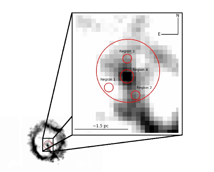
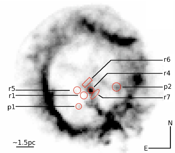
We assume the proper motion center (R.A. 01h04m02, decl. -72∘01’5499 (J2000)) determined in Finkelstein et al., (2006) for the center of our TSR. The physical distance between this center and the main ejecta shell of the remnant is approximately 6 pc. Thus, a “kicked” stellar remnant with the aforementioned properties could not have reached the remnant shell in the expansion lifetime. With the assumption of the Finkelstein et al., (2006) center, we define the TSR as a generous circular area with a radius 1.2 pc, which we overlay on the map of the remnant in Figure 1.
4.1.2 Galactic Analogs to an E0102 Central Compact Stellar Object
In the photometric analysis we perform here, we restrict our search for a stellar object in the remnant to two well-studied potential analogs the central compact object (CCO) in Cassiopeia-A (see Chakrabarty et al., , 2001; Fesen et al., , 2006; Pavlov & Luna, , 2009, and references therein) and the Crab pulsar (see Hester, , 2008, and references therein).
Gaetz et al., (2000) provide an upper limit to the X-ray luminosity of 910erg s-1 for a Crab-like pulsar in the remnant. This limit was determined from a 9.7 ks observation of the remnant with the Chandra ACIS instrument. Further, the spectroscopic study of this remnant by Flanagan et al., (2004) implies that if a Crab-like compact stellar object is present, then it must be faint at X-ray wavelengths.
If the E0102 supernova event generated a Crab-like pulsar, then this object’s spectral behavior would be well described by a power-law, with an approximately constant photon index () in the Chandra bandpass. For the Crab pulsar, 1.6 - 1.8, but the spectrum of the Crab remnant is softer and better fit with 2.0 (Weisskopf et al., , 2004; Seward et al., , 2006). At low energies (energy 0.2 - 2.0 keV), the relative strength of a thermal emission component arising from the remnant plasma is likely to overwhelm the contribution from the Crab-like pulsar component. But, at higher energies, the relative strength of the Crab-like component would increase, possibly to the extent that the compact object could dominate the emission in the center of the remnant, as was observed for the pulsar wind nebula associated with SNR G292+1.8 (Hughes et al., , 2001).
To identify such a trend for this remnant, we first processed the merged image to isolate high and low energy emission between 0.5 and 10.0 keV within energy bins whose widths were selected to include the following known complexes of metal emission-lines of oxygen (O VII triplet 0.46 – 0.6 keV and O VIII Ly 0.61 – 0.72 keV), neon (Ne IX triplet 0.86 – 0.98 keV and Ne X Ly 0.98 – 1.10 keV), magnesium (Mg XI triplet 1.32 – 1.4 keV and Mg XII Ly 1.45 – 1.53 keV); those energies which provide upper and lower energy bounds for each of the previous line complexes (which could be used to identify continuum sources), i.e., a lower bound to oxygen (“Bin 1” energy 0.20–0.40 keV), a lower bound to neon and upper bound to oxygen (“Bin 2” energy 0.75–0.85) and a lower bound to magnesium and upper bound to neon (“Bin 3” energy 1.15–1.275 keV); and the hard (2.0–8.0 keV) continuum. We visually inspected the resulting X-ray spatial flux maps for each of these energy bins, but did not identify a compact object. A Crab-like pulsar should, in addition, be detected across a long wavelength baseline, but the aforementioned studies of E0102 in the radio, optical, and infrared wavelengths have not detected a neutron star. For these reasons, it is unlikely that a Crab-like neutron star is present in this remnant, and for the photometric analysis in this section we consider exclusively the presence of a Cas-A-like CCO.
Chakrabarty et al., (2001) combined ks of Chandra ACIS (S3 chip) observations of Cas-A, determined the location of the compact stellar object, and modeled the luminosity of a neutron star for the remnant. The energy of the maximum count rate for this object peaked at 1.6 keV and was well-fit with an ideal blackbody energy distribution (kT = 0.5 keV), assuming a column density = 1.1 1020 . The X-ray luminosity of the Cas-A CCO is equal to = 2.0 1033 erg s-1. Artificially moving this object to the distance of E0102 (59 kpc), the unabsorbed flux in the same bandpass equals 4.710-15 erg s-1 , or equivalently a count rate equal to 7.1510-4 counts s-1. In 324 ks, this count rate is equivalent to 221 counts. We cannot visually identify a compact object, with this count rate, within the TSR.
An examination of the emission from the remnant within the TSR does reveal a strong gradient in the surface brightness, though. In Figure 1, Region 1 contains an area within which the emission is of the lowest mean surface brightness within the TSR. In this 324 ks exposure, the mean count number within this class of region equals 117. The Q-spoke, the hot extended plasma feature extending from the proper motion center to the shell of the remnant, falls within the TSR and defines a “medium” class of surface brightness regions with average count rates 5 times greater than the low surface brightness regions previously discussed. Regions 2 (mean count 521) and 3 (mean count 459) are regions representative of this class of emission. Within a 2 2 square pixel region (center R.A. - 01h04m02, decl.- -72∘015582 (J2000)), the unique location of peak emission within the TSR defines a third class of surface brightness. The mean count value for this region, Region 4, equals 1157 counts. This variation in surface brightness could imply that a point source exists within the remnant but that the remnant’s hot plasma “masks” the emission that arises from the compact object.
If we assume that a neutron star with a spectral behavior similar to the Cas-A CCO is in fact present in this remnant, but is concealed or masked by the X-ray bright plasma along the line of sight, then the observed count rates can be used to produce upper limits to the luminosity of such a neutron star.
We assume a line of sight SMC HI Column Density222The Milky Way Column Density, estimated with the CXC software package COLDEN an online tool accessible at http://cxc.harvard.edu/toolkit/colden.jsp, is low relative to the SMC absorption, with = 6.57 1020 cm-2, = 5.82 1021 cm-2 from Stanimirović et al., (1999). With PIMMS333Available at http://cxc.harvard.edu/toolkit/pimms.jsp, we then calculate the upper limit to the flux, and derive the luminosity, for a Cas-A neutron star with either a blackbody or power-law spectral energy distribution. For these calculations, we set the blackbody kT parameter and the power-law photon index equal to the similar best-fit parameters derived by Chakrabarty et al., (2001). We present these upper limits in Table 2. In this table, the 5 rms sky noise (in counts) is never greater than , which implies less than of the counts for each of the regions in Table 2 are detector, or sky, background not arising from the remnant. We do not attempt here to estimate the background “noise”, within each region, which arises from the remnant plasma directly (see Section 4.2).
A compact object is only one of many components contributing to total flux observed within a region of interest, and within the TSR (particularly within Region 4), the contribution from this source may be small relative to other components (background and sky “noise”, detector noise, detector response, absorbers along the line of sight, etc.). Nevertheless, for regions which are not coincident with the Q-spoke, the “zeroth-order” estimates to the upper limits to the flux from a compact object in these regions may be reasonable, as the contribution of a compact object in one of these regions cannot, by definition, exceed the observed flux. But, the TSR includes bright emission from the Q-spoke, and the surface brightness variations indicate that the contribution of the remnant plasma is variable with position. Thus, quantifying the contribution of a compact object to the total observed flux for each region requires a more rigorous estimation of the contribution of the background to the total observed flux. In the following sections, we present the results of two methods which provide a more robust determination of the relative strength of a compact object within the TSR.
4.1.3 Point-source Identification
To date no study of E0102 has reported the detection of a compact object in physical association with the remnant. But, previous investigations of E0102 were limited in their sensitivity and spatial resolution. Combining the extensive archived observations of this remnant, we have produced a high signal-to-noise image of the remnant, at the superior X-ray spatial resolution of the Chandra ACIS instrument suite, which represents the best opportunity to identify a compact object within the TSR, particularly in the vicinity of Region 4.
In the previous section, it was found that complex surface brightness variations (with radius, measured from the center of the remnant) prevent any conclusive visual identification of a compact object. In this section, we search for a point-source object in the image using the CIAO wavdetect script, which is the optimal source detection software package for Chandra X-ray images. This software iteratively identifies source objects by correlating image pixels with “Mexican Hat” wavelets, for a selection of user-defined wavelet scales(for a description of the software, see Freeman et al., , 2002). We apply wavdetect for source detection in seven images of the remnant Broad (energy 0.5–7.0 keV), Medium (energy 1.2–2.0 keV), Soft (energy 0.5–1.2 keV), Hard (energy 2.0–7.0 keV)444These first four energy bands are directly comparable to Chandra Source Catalogue bands., and the three energy bands discussed in Section 4.1.2 that selected continuum emission between strong line complexes. For each of these images, wavdetect was used to identify sources on “Fine” (scales = “1 2”) and “Coarse” (scales = “4 8 16”) scale, with sigthresh555sigthresh defines the threshold at which “cleaned” pixels are considered to be members of a source detection set equal to 410-5. We ran each wavdetect search twice, with and without an effective exposure map, and found the same number of detections within the TSR.
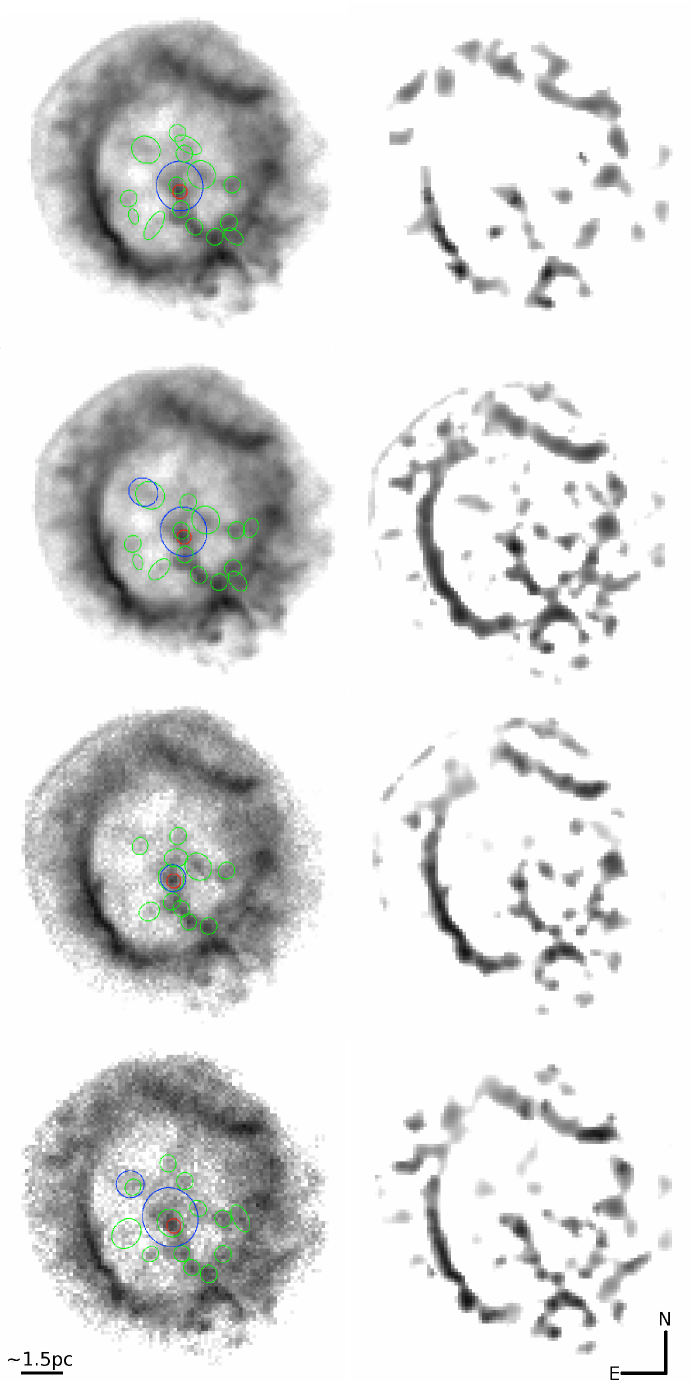
wavdetect searches in each of these images identified a source within Region 4, and the detection ellipse for each of these sources included part (or all) of this region. In Figure 2, we overplot the source detections which were identified within 100 of the expansion center for the Broad, Hard, “Bin 2” and “Bin 3” continuum images. In addition, we include in Figure 2 the “image file”, an output from the wavdetect routine that is a representation of the data with background and noise subtracted. We are reluctant to conclude that these source detections are associated with a compact object, though, and believe that these results reinforce, quantitatively, the preliminary conclusion presented in Section 4.1.2 that a compact object may be present in or near to the brightest pixel region (Region 4) but masked, for the following reasons.
First, the wavdetect results confirm that the Q-spoke is a real feature, contributes significantly to surface brightness variation across the center of the remnant, runs continuously between the center and outer edge (from the observer’s perspective) of the remnant as illustrated in the “image file”, and the brightest pixel region remains “masked” in the Q-spoke in the “image file”.
wavdetect provides a variety of photometric measurements which can be used to constrain the extended versus compact nature of detected objects (e.g., PSFRATIO666wavdetect calculates this by dividing the estimated “radius” of the source cell to PSF_SIZE, an estimate of the point-spread function (PSF) calculated at the location of the detection. For further information, please see the CIAO Detect Reference Guide at http://cxc.harvard.edu/ciao/download/doc/detect_manual/wav_ref.html) and an estimate to the statistical significance of each detection (SRC_SIGNIFICANCE777wavdetect provides an estimate to the significance of the detection with respect to the calculated background for the source detection region, but should not be taken at face value. This statistic is defined in the CIAO Detect Reference Guide and is calculated by dividing the net counts by the “Gehrels error”, .). When the source detections nearest to the brightest pixel region are considered individually, these statistical measurements could suggest possible point source detections, particularly in the narrow band images. Considered in the context of the full set of detections, though, the sources detected in the proximity of Region 4 are indistinguishable from other detections within the remnant, most of which are associated with hot gas background emission that could not be reduced from the image file by the wavdetect software. Furthermore, the lack of nearby point sources or double-peaked source detections make it difficult to interpret these results. In Table 3 we provide pertinent statistics for the set of detections from each of the wavdetect searches; here, we limit the set to those which have detection ellipse centers () interior to the outer shell of the remnant.
Lastly, each image’s source detection ellipse most closely matching to, or including Region 4, in the “Fine”-scale wavdetect search is found to be offset from the center of Region 4 by less than 10. But the size of the detection ellipse significantly increases at the “Coarse” scale. These latter two results likely indicate the difficulty which wavdetect has in adequately discriminating between sources and unresolved background components, or knots of hot plasma and “masked” compact objects.
Though the wavdetect search results provide more point source candidates within the TSR, we believe that any photometric method of estimating the relative strength of a compact object “masked” by the Q-spoke is inadequate and now turn to a spectral analysis for characterizing the background emission.
4.2 Spectral Analysis
In the previous sections, we were limited in deriving firm upper limits on the detection and characterization of a compact object by the presence of a high surface brightness emission component that likely arises from the remnant plasma. In this section, we perform a spectral analysis designed to quantify the contribution of multiple background components present within an expanded set of regions within or near to the TSR. Only by fitting and reducing out the contribution of these components in the regions of interest will we be able to conclude firm upper limits for compact objects which may be masked by the Q-spoke.
It is necessary to note that E0102 is used by the Chandra facility as a spectral calibration source, because it is a relatively constant and bright X-ray source, especially at energies between 0.55 and 0.7 keV corresponding to the emission-lines of O VII and O VIII. As such, it is an optimal target for use in calibrating the response of the ACIS CCDs and the variability of these CCDs response in time (see, e.g., Plucinsky et al., (2008)). Imaging of the remnant for calibration purposes does not preclude us from searching for multiple additional spectral components, though.
Using the CIAO script specextract, we extracted spectra for each of the regions discussed in Section 4.1 (see Figure 1) and an additional six regions of varied size, shape, and location. We select these regions to better characterize the background emission within the remnant, not just within the Q-spoke and TSR. In Figure 3, we provide a map of the regions, interior to the remnant shell, for which spectra were extracted. Not displayed in Figure 3 is the background region (area 27,000 pixel2) which was used to characterize the X-ray sky background not originating from the remnant itself. These regions were selected from areas of the chip where the individual ObsID exposures were, when stacked, spatially coincident at distance well beyond the remnant. For legibility, Figure 3 does not include Regions 2 and 3.
In this section, we are concerned exclusively with the detection of a point source object by its spectral signature. In theory, the detection of any such object is possible only by identifying and reducing, from the spectral profile extracted for a particular region of interest, all emission which does not arise from the point source itself so that the flux from the compact object can be properly measured. We assumed that this background arose from one of three sources the X-ray background sky arising from astrophysical sources independent of the remnant as well as instrumental background particular to the ACIS detector (i.e., “chip noise”), which we will refer to here as “Component A” background, and diffuse emission arising from E0102 ejecta, the intensity of which varies with the position in the remnant, which we will refer to as “Component B” background.
To calibrate the emission arising from the X-ray sky (e.g., diffuse galactic Milky Way and SMC emission), and the background arising from the ACIS detector electronics (e.g., the well-understood fluorescence lines of Si K, Al K, etc.; Baganoff 1999), we first analyzed a spectrum extracted from a uniform region (the aforementioned “background region”) located approximately 1’ from the outermost radial extent of the remnant. Using the xspec888see http://heasarc.gsfc.nasa.gov/docs/xanadu/xspec/ software package, we then modeled the broadband spectral behavior of this “Component A” emission using multiple power-law and Gaussian components to represent this diffuse X-ray sky emission and lines. With 583 degrees of freedom in the model fit to “Component A” background emission, the reduced minimized statistic for the best-fit model is equal to 1.03. For this analysis, and throughout this section, we consider the spectral profile in two energy bins, “soft” X-rays (0.5 – 2.0 keV) and “hard” X-rays (2.0 – 8.0 keV ).
“Component A” background emission is assumed to be uniformly present and of similar intensity within each of the regions for which we extracted spectra. This assumption does not hold for “Component B” emission which arises from the remnant itself. To fit this class of background emission, we must consider each of the spectra individually. Because our goal is to identify a spectrally distinct compact object in this remnant, we aim to characterize the diffuse plasma spectrum rather than to physically understand it. Therefore, we fit an ad hoc model to the spectrum for each of the regions. Again, we used the xspec package to model this background emission, fitting the “Component B” X-ray emission (which was dominated, not unexpectedly, in the soft band by the strong oxygen and neon emission-line complexes) with a system of Gaussian line profiles, and also with a variable APEC model (see Smith et al., , 2001). We acknowledge here that the spectral resolution is insufficient for distinguishing between spectral lines and continuum emission between those lines; thus the fits to these sources of background emission are model dependent. Therefore, in the following analysis, the upper limits to the continuum emission from any putative neutron star are implicitly model dependent.
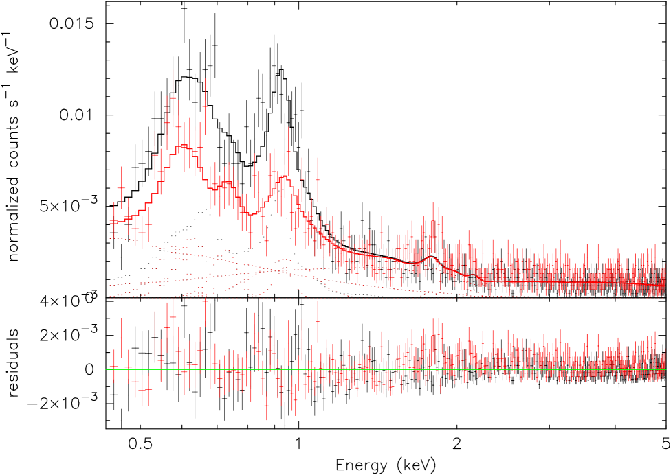
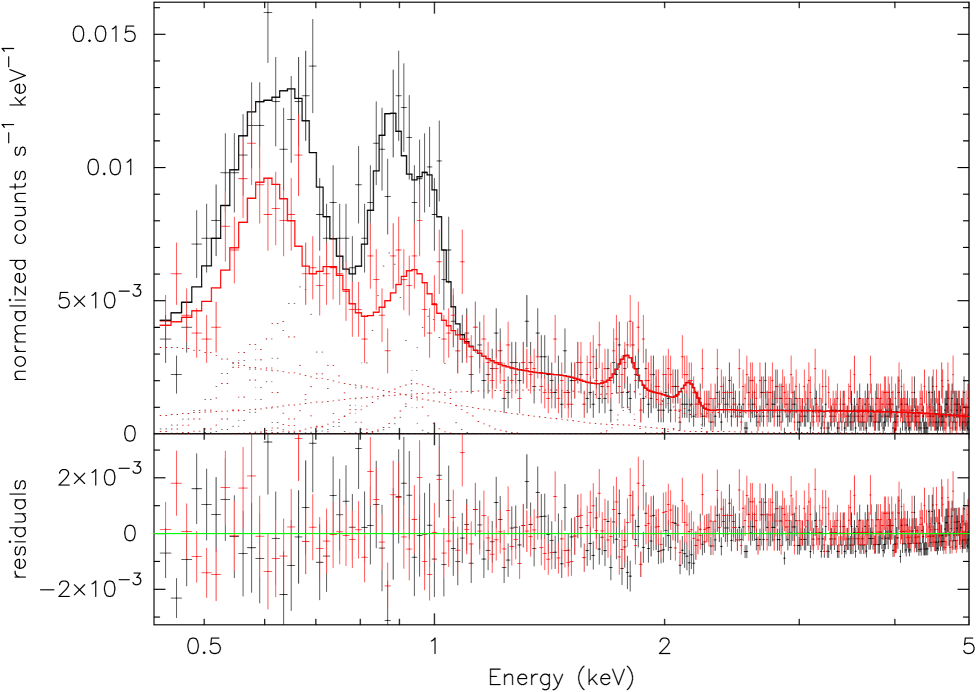
For each region, we combine both background models generated to produce a unified background model which we then fit to each of the observed spectra. In Figure 4, we present the unified background model in its component form. In this figure, black data points with error bars represent the observed imaging spectrum extracted from, in this example, the brightest pixel region (Region 4). The “Component A” background model fit is overplotted in red the red solid curve represents the sum of the individual model components (red dotted line) fit to the red observed data points (plotted with error bars) of the extracted spectrum from the background region. The unified background model, which includes the region-specific “Component B” background emission, is overplotted in black; in this figure the Component B emission model was generated using a variable APEC model and power-law components. For comparison, we provide in Figure 5 the background model fit, but with “Component B” emission-line complexes modeled with a system of Gaussian spectral lines. Each model reproduces the observations well, within the given errors, but in general the vAPEC models have smaller residuals.
The best-fit background model was determined for each of the extracted spectra by iteratively minimizing the statistic. The “Minimum ” value for each best-fit unified background model is provided in Table 4. Each model, for both the vAPEC and Gaussian fits, was defined with 577 degrees of freedom, thus the reduced for each of the background fits was 1.0 (e.g. Region 4, ). As “Component A” background emission was fixed in its contribution to the spectral energy distribution extracted for each region, this figure of merit essentially measures the goodness of the fit of “Component B” background emission, which arises predominantly from nebular line emission.
Having sufficiently accounted for all sources of background emission, we can then derive an upper limit to the presence of a compact object within each of the regions. To derive these upper limits, we assume that a compact object is a neutron star and is well described by either a power-law or a blackbody model (hereafter, referred to as the “point-source model”).
We define the point-source model as the product of a normalization constant and the specific functional form; for example, the power-law model point-source model function is . Combining the best-fit unified background model, now fixed for each region by the previous analysis, with the point-source model, we define a two-component spectral model which we then re-fit to the observed spectrum for each region by only varying the magnitude of the normalization constant 999We fix (or kT, in the case of the Blackbody point source model) for each fit.. We increase the strength of the point-source component in this two-component model only until is no longer satisfied. Note that 6.63 is the chi-square difference constant implying an observation is significant at the 99% (3 ) confidence level for a system modeled with 1 degree of freedom. Thus, with this analysis we have measured the upper limit to the observed flux from a compact stellar object, above which such an object would have been detected in this data.
In Table 4 we present the results of this analysis, which we completed for three power-law models of a compact stellar object defined with set equal to 1, 3, and 5, respectively. This range of indices spans the observable parameter space for the Cas-A CCO (power-law fit, see Pavlov & Luna, , 2009) and pulsars (i.e., the Crab pulsar). In Columns 2 – 6 of Table 4 we present the flux, equivalent luminosity, and the minimum statistic we determine from the best-fit unified background model to the spectrum extracted for each regions. In Columns 8–13 we present the upper limits to a neutron star for E0102. Specifically, in Columns 8 and 11, we present the flux difference between the two component best-fit model and the unified background fit for the region, for the soft and hard energy bands respectively. Positive values in both the soft and hard energy bands indicate that the normalization parameter that was found to satisfy the statistical criterion (defined previously) in one band, simultaneously satisfied the criterion in the other band. Or, similarly, the point-source model flux in both bands was sufficiently greater than the unified background model to be detected, minimally at 99% confidence. Negative or zero values in Columns 8 and 11 should be interpreted as non-detections at the 99% confidence level. These non-positive values can be attributed to a lack of discriminatory power in the models for differentiating between remnant hot gas emission and the point source component, within the observational errors, at the confidence level defined by the statistical criterion. The remnant is dominated by soft emission; thus these non-detections typically arise for the softest ( = 5) point source component model fits. We could produce upper limits for these models if we instead chose to enforce a stricter confidence level, e.g. 99.5%, which would require us to redefine the statistical criterion (in this example, ). Lastly, in Columns 9 and 12 we present the flux upper limits, and in Columns 10 and 13 we present the equivalent luminosity upper limits for the stellar object.
Because the brightest pixel region (Region 4 in Figure 2) has a distinct photometric signature (see Sections 4.1.2 and 4.1.3), we perform a similar analysis to that which was outlined above for this region, but also explore the possibility that the point source component within the two component model is best described by a blackbody model. We present this analysis for both the power-law ( = 1, 3, and 5) and Blackbody (kT = 0.25, 0.5, and 1.0) model point source components in Table 5.
5 Discussion
We interpret the non-detection of a compact stellar object in the remnant E0102 within the context of three physical scenarios. In the first of these scenarios, the non-detection of a compact stellar object for E0102 implies that such an object simply does not exist. There are two plausible scenarios to consider when addressing this possibility.
First, a stellar compact object may have been destroyed during the supernova event. If E0102 represents the end stage of a Type Ia supernova event, then the progenitor white dwarf(s) would have likely been destroyed (Woosley et al., , 1986). But, it is difficult to reconcile this formation scenario with the evidence presented by Blair et al., (2000) and Chevalier, (2005) which would support a Type Ib/c or IIb/L class supernova event for the E0102 progenitor.
The theory of Type Ib/c and Type II supernova predicts that compact objects are generated during the supernova event, and compact stellar objects have been observed in physical association with 25% of Galactic remnants (see Green’s Catalogue; G06). But, in addition to these neutron-degenerate stellar objects, core-collapse supernovae of sufficiently massive ( 20) progenitors may generate black holes (see Smartt, , 2009, for a review). At least two arguments exist in support of the black hole scenario, and though they are circumstantial they should be addressed in future work on the remnant. First, Finkelstein et al., (2006) suggest that E0102’s progenitor star may have been a massive (50 M⊙) Wolf-Rayet star, based on the consideration of the local environment of the remnant. Second, to explain a similar remnant morphology in the SNR W49B, Keohane et al., (2007) suggest a possible jet-driven explosion mechanism (a “collapsar” model; McFadyen et al., , 2000), which would generate a black hole.
A second interpretation of the non-detection of a compact stellar object in the remnant is that a neutron star in this remnant is in fact present, but is both faint in its emission and obscured by the Q-spoke. This possibility is motivated by the imaging and analysis presented in Sections 4.1.2, 4.1.3, and 4.2.
A final interpretation of the non-detection of a compact stellar object is systemic, such that the estimate to NH is too low. Thus, the flux from a compact object in this remnant is absorbed by the interstellar medium (ISM) along the line of sight. At a distance of 59 kpc, the Cas-A CCO would have a detectable signal; in this 324 ks ACIS image, this signal would be equivalent to 240 counts between the energies of 0.1 and 10 keV. Such a source would stand well above the noise in this observation. But, the average number count within that portion of the TSR unobscured by the Q-spoke is equal to 140 in the 324 ks exposure. By measuring the relative strength of the background in an image filtered for energies greater than 10 keV (above which the effective area of Chandra ACIS is nominally zero with respect to the known background for the S3 chip), an estimate to the cosmic ray background count rate can be made. With this rate appropriately scaled to the exposure length and area of this region, it can be shown that only a small fraction of these counts ( 1 %) can be attributed to cosmic rays. Thus, to reduce the Cas-A-like neutron star flux to this observed level would require a column density along the line of sight 12 times higher than we assumed. This is not reasonable given the errors on NH, and we conclude that gas along the line of sight is not likely to obscure the flux from a compact object in this remnant.
The non-detection of a compact object for this remnant, though, does not preclude its detection at shorter or longer wavelengths than the Chandra operational energy bands. In particular, this research suggests that imaging of the remnant at those wavelengths at which emission from ejecta material is relatively low may reveal such an object. Recently, Camilo et al., (2009) presented the detection of a radio pulsar in association with Galactic SNR G315.9-0.0. This remnant displays a similar emission “spoke,” extending perpendicularly outward from the remnant, with the radio pulsar detected at the outermost tip of Q-spoke. The remnant E0102 and G315.9-0.0 should not be directly compared because of morphological differences and different estimated ages, but the results of Camilo et al., (2009) and this research suggests that a more extensive review at radio wavelengths could provide insight into the nature of a compact object for this remnant. Furthermore, the recent result of 16 galactic pulsars discovered with the Fermi Gamma Ray Telescope (Abdo et al., , 2009) suggests that imaging of the remnant at higher energies than the Chandra bands may be fruitful. In addition, a high- resolution timing study of the center of the TSR could detect a pulsar. At present, Chandra GO program 11500201 (PI Petre) is approved for 20 ks of imaging with HRC-I in Spring 2010. These data could be used in the assessment of temporal variability of an, as of yet, undetected central pulsar.
6 Conclusion
We have combined 324 ks of Chandra X-ray observations of the SNR 1E0102.2—7219 in the SMC to produce the highest signal-to-noise image of this young, oxygen-rich remnant. In this research, we attempt to identify a compact stellar object for this remnant within a generous search area motivated by observations of this remnant, Galactic SNRs, and compact stellar objects. We cannot confirm the presence of a compact object for this remnant, but are able to provide the strongest upper limits on the flux, assuming that the spectral behavior of a faint neutron star for this remnant is best described by a blackbody or power-law spectrum energy distribution.
7 Acknowledgments
This research has made use of data obtained from the Chandra Source Catalog, provided by the Chandra X-ray Center (CXC) as part of the Chandra Data Archive. This research was partly funded by the Arizona State University—NASA Space Grant program. M. Rutkowski recognizes the Harvard-SAO Summer Research Experience Program for Undergraduates. The authors thank an anonymous referee for comments that significantly improved the manuscript.
References
- Abdo et al., (2009) Abdo, A. A., et al. 2009, Science, 325, 840
- Amy & Ball, (1993) Amy, S. W., & Ball, L. 1993, ApJ, 411, 761
- Baganoff, (1999) Baganoff, F., ACIS On-orbit Background Rates and Spectra from Chandra OAC Phase 1 (ACIS Memo No. 162; Cambridge, MA: MIT Center for Space Research)
- Blair et al., (1989) Blair, W. P., Raymond, J. C., Danziger, J., & Matteucci, F. 1989, ApJ, 338, 812
- Blair et al., (2000) Blair, W. P., et al. 2000, ApJ, 537, 667
- Camilo et al., (2009) Camilo, F., et al., 2009, ApJ, 703, L55
- Chakrabarty et al., (2001) Chakrabarty, D., et al., 2001, ApJ, 548, 800
-
Chandra Proposers’ Observatory Guide, (2009)
Chandra Proposers’ Observatory Guide, v. 12.0, 2009
available at http://cxc.harvard.edu/proposer/POG/ - Chevalier, (2005) Chevalier, R. A., 2005, ApJ619, 839
- Eriksen et al., (2001) Eriksen, K. A., Morse, J. A, Kirshner, R. P., and Winkler, P. F., 2001, in AIP Conf. Proc. 565, Eleventh Astrophysics Conference, College Park, Maryland, 2000, Young Supernova Remnants, ed. S.S. Holt & U. Hwang (Melville, NY AIP), 193
- Fesen et al., (2006) Fesen, R. A., Pavlov, G. G., Sanwal, D., 2000, ApJ, 646, 838
- Finkelstein et al., (2006) Finkelstein, S. L., et al. 2006, ApJ, 641, 919
- Flanagan et al., (2004) Flanagan, K. A. et al. 2004, ApJ, 605, 230
- Fragos et al., (2009) Fragos, W., et al., 2009, ApJ, 697, 1057
- Freeman et al., (2002) Freeman, P. E., Kashyap, V., Rosner, R., & Lamb, D. Q., 2002, ApJS, 138, 185
- Fryer et al., (2006) Fryer, C. & Kusenko, A. 2006, ApJS,163, 335
- Gaetz et al., (2000) Gaetz, T. J., et al., 2000, ApJ, 534, L47
- Garmire et al., (2003) Garmire, G. P., et al., 2003, Proc. SPIE, 4851, 28
- Hayashi et al., (1994) Hayashi, I., et al., 1994, PASJ, 46, L121
- Hester, (2008) Hester, J. J., 2008, ARA&A, 46,127
- Hobbs et al., (2005) Hobbs, G., Lorimer, D. R., Lyne, A. G., & Kramer, M. 2005, MNRAS, 360, 974
- Hughes et al., (2000) Hughes, J. P., Rakowski, C. E., & Decourchelle, A. 2000, ApJ, 543, L61
- Hughes et al., (2001) Hughes, J. P., et al., 2001, ApJ, 559, L153
- Keohane et al., (2007) Keohane, J. W., Reach, W. T., Rho, J., & Jarrett, T. H 2007, ApJ, 654, 938
- Li et al., (2003) Li, J., Kastner, J. H., Prigozhin, G. Y., & Schulz, N. S. 2003, ApJ, 590, 586
- McFadyen et al., (2000) MacFadyen, A. I., Woosley, S. E., & Heger, A. 2000, ApJ, 550, 410
- Pavlov & Luna, (2009) Pavlov, G. G. & Luna, G. J. M. 2009, ApJ, 703, 910
- Plucinsky et al., (2008) Plucinsky, P. P., et al. 2008, in Proc. SPIE Vol. 7011, Space Telescopes and Instrumentation 2008 Ultraviolet to Gamma Ray, ed. Turner, M.J.L. & Flanagan, K.A. (Marseille, FRANCE SPIE) 68
- Rasmussen et al., (2001) Rasmussen, A. P., Behara, E., Kahn, S. M., den Herder, J. W., & van der Heyden, K. 2001, A&A, 365, L231
- Seward & Mitchell, (1981) Seward, F. D., & Mitchell, M., 1981, ApJ, 243, 736
- Seward et al., (2006) Seward, F D., Tucker, W. H., & Fesen, R. A. 2006, ApJ, 652, 1277
- Smartt, (2009) Smartt, S. J. 2009, ARA&A, 47, 63
- Smith et al., (2001) Smith, R. K., Brickhouse, N. S., Liedahl, D. A., Raymond, J. C., 2001, ApJ, 556, L91
- Stanimirović et al., (1999) Stanimirović S., Staveley-Smith, L., Dickey, J. M., Sault, R. J. & Snowden, S. L. 1999, MNRAS, 302, 417
- Stanimirović et al., (2005) Stanimirović S., et al., 2005, ApJ, 632, 103
- Tuohy & Dopita, (1983) Tuohy, I. R. & Dopita, M. A. 1983, ApJ, 268, L11
- van den Bergh, (1999) van den Bergh, S. 1999 in IAU Symp. 190, New Views of the Magellanic Clouds, ed. Y.-H. Chu, N. Suntzeff, J. Hesser, & D. Bohlender (San Francisco, CA: ASP), 569
- Wang & Wheeler, (2008) Wang, L., & Wheeler, J. C. 2008, ARA&A, 46, 433
- Weisskopf et al., (2004) Weisskopf, M. C., et al. 2004, ApJ, 601, 1050
- Woosley et al., (1986) Woosley, S. E., Taam, R. E., & Weaver, T. A. 1986, ApJ, 301, 601
| Year | Exposure Time (ks) | ObsIDs |
|---|---|---|
| 2000 | 35.00 | 1308, 1423, 1803 |
| 2001 | 32.48 | 141, 1311, 2843, 2844 |
| 2002 | 15.33 | 2850, 2851 |
| 2003 | 51.70 | 3519, 3544, 5123, 5251, 5252 |
| 2004 | 55.12 | 5130, 5131, 6074, 6075 |
| 2005 | 26.75 | 6042, 6043 |
| 2006 | 53.30 | 6758, 6759, 6765, 6766 |
| 2007 | 20.98 | 8365 |
| 2008 | 19.20 | 9694 |
| 2009 | 14.57 | 10655, 10656 |
| Region11For the location of each region, see Figure 1; 2 in counts s-1; 3 Unabsorbed (0.1-10 keV) Flux [erg s-1 cm-2] derived from Observed count rate, and calculated by PIMMS assuming Cycle 10 systematics for ACIS-S with no gratings; 4 Unabsorbed Luminosity [erg s-1]; 5 Estimate of the Unabsorbed Luminosity from previous column, Unabsorbed Luminosity determined by Chakrabarty et al., (2001). | Count Rate22“Fine” wavdetect “scale” parameter “1 2”; “Coarse” wavdetect parameter “scale” “4 8 12”. | Flux 33wavdetect parameter PSFRATIO which can be used identifying extended sources; see Section 4.1.3. | Luminosity 44wavdetect parameter SRC_SIGNIFICANCE; see Section 4.1.3. | 55Number of detections within 25 of the E0102 expansion center. | Flux | Luminosity | ||
|---|---|---|---|---|---|---|---|---|
| Assume 2.35 | Assume 3.13 | |||||||
| 1 | 3.61 (–4) | 1.12 (–14) | 4.65 (33) | 0.62 | 3.73 (–14) | 1.55 (34) | 0.35 | |
| 2 | 1.61 (–3) | 5.01 (–14) | 2.09 (34) | 2.81 | 1.66 (–13) | 6.89 (34) | 1.60 | |
| 3 | 1.41 (–3) | 4.39 (–14) | 1.82 (34) | 2.46 | 1.46 (–13) | 6.06 (34) | 1.41 | |
| 4 | 3.57 (–3) | 1.11 (–13) | 4.61 (34) | 6.22 | 3.69 (–13) | 1.53 (35) | 3.56 | |
| Assume kT=0.53 | Assume kT=0.49 | |||||||
| 1 | 3.61 (–4) | 3.49 (–15) | 1.45 (32) | 0.85 | 3.46 (–15) | 1.44 (33) | 0.72 | |
| 2 | 1.61 (–3) | 1.56 (–14) | 6.47 (33) | 3.81 | 1.55 (–14) | 6.43 (33) | 3.21 | |
| 3 | 1.41 (–3) | 1.37 (–14) | 5.69 (33) | 3.34 | 1.35 (–14) | 5.60 (33) | 2.80 | |
| 4 | 3.57 (–3) | 3.46 (–14) | 1.44 (34) | 8.45 | 3.43 (–14) | 1.42 (34) | 7.12 | |
Note. — (–k) is equivalent to
| Band11See Sections 4.1.2 and 4.1.3 for energy band definitions. | Search Scale22“Fine” wavdetect “scale” parameter “1 2”; “Coarse” wavdetect parameter “scale” “4 8 12”. | PSF Ratio33wavdetect parameter PSFRATIO which can be used identifying extended sources; see Section 4.1.3. | Significance44wavdetect parameter SRC_SIGNIFICANCE; see Section 4.1.3. | 55Number of detections within 25 of the E0102 expansion center. | PSF Ratio66Mean, and 1 variance from mean, of wavdetect parameter PSFRATIO for all detections () in energy band. | Min. PSF Ratio77Minimum PSFRATIO value for source detection interior to E0102. | Significance66Mean, and 1 variance from mean, of wavdetect parameter PSFRATIO for all detections () in energy band. | Max. Significance88Maximum SRC_SIGNIFICANCE value for source detection interior to E0102. | |
|---|---|---|---|---|---|---|---|---|---|
| Nearest Detection99Detection nearest, in proximity, to Region 4. | Remnant Detections | ||||||||
| Broad | Coarse | 5.72 | 176.4 | 11 | 6.9 2.1 | 3.41 | 544 259 | 922 | |
| Fine | 1.98 | 98.5 | 93 | 2.2 0.8 | 1.6 | 31 32 | 132 | ||
| Soft | Coarse | 5.73 | 159.9 | 10 | 7.1 1.8 | 3.46 | 556 212 | 887 | |
| Fine | 1.95 | 48.2 | 91 | 2.1 0.8 | 1.4 | 31 32 | 139 | ||
| Hard | Coarse | 5.56 | 16.4 | 15 | 6.0 2.3 | 5.10 | 38 19 | 76 | |
| Fine | 1.95 | 8.1 | 31 | 2.2 0.7 | 1.75 | 6 2 | 10 | ||
| Medium | Coarse | 6.85 | 130.4 | 13 | 6.9 2.0 | 3.42 | 172 74 | 302 | |
| Fine | 3.21 | 36.7 | 76 | 2.4 0.8 | 1.8 | 15 10 | 45 | ||
| “Bin 1” | Coarse | 7.17 | 11.5 | 11 | 7.1 2.01 | 3.09 | 51 17 | 79 | |
| Fine | 1.96 | 6.4 | 26 | 1.8 0.9 | 1.8 | 6 3 | 14 | ||
| “Bin 2” | Coarse | 3.11 | 47.7 | 10 | 7.2 2.3 | 3.11 | 187 71 | 308 | |
| Fine | 3.13 | 29.6 | 67 | 2.2 0.8 | 1.8 | 15 11 | 46 | ||
| “Bin 3” | Coarse | 6.83 | 44.4 | 11 | 6.9 1.9 | 4.74 | 107 47 | 172 | |
| Fine | 3.20 | 23.3 | 63 | 2.1 0.9 | 1.4 | 10 6 | 30 | ||
| Region | ††Modeled background flux “s” designates the soft X-ray band ( 0.5 – 2.0 keV ) and “h” designates the hard X-ray band ( 2.0 – 8.0 keV ) modeled flux (erg s-1 cm-2) — ††Equivalent background luminosity, assuming distance to E0102 equal to 59 kpc; “s” designates the soft X-ray band ( 0.5 – 2.0 keV ) and “h” designates the hard X-ray band ( 2.0 – 8.0 keV ) modeled flux (erg s-1 cm-2) — ‡Minimum , =577; please see Section 4.2 — a Assumed Power Law Index, — b the difference between the modeled unified background flux and the flux of the model point source, in energy band x — c the point source upper flux limit, in energy band x — d the equivalent point source upper luminosity, in energy band x | ††††footnotemark: | Min. ‡‡footnotemark: | , Photon Indexaafootnotemark: | bbfootnotemark: | ccfootnotemark: | ddfootnotemark: | ||||||
|---|---|---|---|---|---|---|---|---|---|---|---|---|---|
| Background Fit | Point Source Fit | ||||||||||||
| p1 | 2.167 (–14) | 8.992 (33) | 2.433 (–13) | 1.010 (35) | 1.07 | 1 | 9.600 (–16) | 2.263 (–14) | 9.391 (33) | 3.800 (–15) | 2.471 (–13) | 1.025 (35) | |
| 3 | 9.000 (–16) | 2.257 (–14) | 9.366 (33) | 2.000 (–16) | 2.435 (–13) | 1.010 (35) | |||||||
| 5 | 3.600 (–16) | 2.203 (–14) | 9.142 (33) | 0.000 | 2.433 (–13) | 1.010 (35) | |||||||
| p2 | 2.202 (–14) | 9.138 (33) | 2.407 (–13) | 9.988 (34) | 1.05 | 1 | 7.900 (–16) | 2.281 (–14) | 9.465 (33) | 3.100 (–15) | 2.438 (–13) | 1.011 (35) | |
| 3 | 7.300 (–16) | 2.275 (–14) | 9.441 (33) | 1.000 (–16) | 2.408 (–13) | 9.992 (34) | |||||||
| 5 | -1.500 (–16) | 2.187 (–14) | 9.075 (33) | 8.900 (–15) | 2.496 (–13) | 1.036 (35) | |||||||
| r1 | 2.185 (–14) | 9.067 (33) | 2.443 (–13) | 1.014 (35) | 1.08 | 1 | 8.200 (–16) | 2.267 (–14) | 9.407 (33) | 3.300 (–15) | 2.476 (–13) | 1.027 (35) | |
| 3 | 9.000 (–16) | 2.275 (–14) | 9.441 (33) | 2.000 (–16) | 2.445 (–13) | 1.015 (35) | |||||||
| 5 | 3.600 (–16) | 2.221 (–14) | 9.216 (33) | 0.000 | 2.443 (–13) | 1.014 (35) | |||||||
| r2 | 2.222 (–14) | 9.221 (33) | 2.457 (–13) | 1.020 (35) | 1.05 | 1 | 8.000 (–16) | 2.302 (–14) | 9.552 (33) | 3.100 (–15) | 2.488 (–13) | 1.032 (35) | |
| 3 | 7.900 (–16) | 2.301 (–14) | 9.548 (33) | 1.000 (–16) | 2.458 (–13) | 1.019 (35) | |||||||
| 5 | 3.600 (–16) | 2.258 (–14) | 9.369 (33) | –1.000 (–16) | 2.456 (–13) | 1.019 (35) | |||||||
| r3 | 2.222 (–14) | 9.221 (33) | 2.357 (–13) | 9.781 (34) | 1.06 | 1 | 8.000 (–16) | 2.302 (–14) | 9.553 (33) | 3.200 (–15) | 2.389 (–13) | 9.913 (34) | |
| 3 | 9.000 (–16) | 2.312 (–14) | 9.594 (33) | 2.000 (–16) | 2.359 (–13) | 9.789 (34) | |||||||
| 5 | 4.200 (–16) | 2.264 (–14) | 9.395 (33) | 0.00 | 2.357 (–13) | 9.780 (34) | |||||||
| r5 | 2.220 (–14) | 9.212 (33) | 2.435 (–13) | 1.010 (35) | 1.05 | 1 | 8.000 (–16) | 2.300 (–14) | 9.544 (33) | 3.200 (–15) | 2.467 (–13) | 1.023 (35) | |
| 3 | 8.900 (–16) | 2.309 (–14) | 9.581 (33) | 2.000 (–16) | 2.437 (–13) | 1.011 (35) | |||||||
| 5 | 3.000 (–16) | 2.250 (–14) | 9.336 (33) | 0.000 | 2.435 (–13) | 1.010 (35) | |||||||
| r6 | 2.213 (–14) | 9.183 (33) | 2.444 (–13) | 1.014 (35) | 1.05 | 1 | 8.100 (–16) | 2.294 (–14) | 9.519 (33) | 3.200 (–15) | 2.476 (–13) | 1.027 (35) | |
| 3 | 8.300 (–16) | 2.296 (–14) | 9.527 (33) | 2.000 (–16) | 2.446 (–13) | 1.015 (35) | |||||||
| 5 | 3.600 (–16) | 2.249 (–14) | 9.332 (33) | 0.000 | 2.444 (–13) | 1.014 (35) | |||||||
| r7 | 2.200 (–14) | 9.129 (33) | 2.339 (–13) | 9.706 (34) | 1.05 | 1 | 8.100 (–16) | 2.281 (–14) | 9.465 (33) | –7.000 (–15) | 2.269 (–13) | 9.416 (34) | |
| 3 | 8.400 (–16) | 2.284 (–14) | 9.477 (33) | –1.000 (–14) | 2.239 (–13) | 9.291 (34) | |||||||
| 5 | 3.900 (–16) | 2.239 (–14) | 9.291 (33) | –1.030 (–14) | 2.236 (–13) | 9.278 (34) | |||||||
Note. — ( – k) is equivalent to
| ††††footnotemark: | ‡‡footnotemark: | Min. ‡‡‡‡footnotemark: | Fixed Parameteraafootnotemark: | bbfootnotemark: | ccfootnotemark: | ddfootnotemark: | |||||||
|---|---|---|---|---|---|---|---|---|---|---|---|---|---|
| Background Fit | Point Source Fit | ||||||||||||
| Blackbody Fit | 2.171 (–14) | 9.009 (33) | 2.309 (–13) | 9.581 (34) | 0.78 | 0.25 | 0.163 (–14) | 2.334 (–14) | 9.685 (33) | 0.001 (–13) | 2.310 (–13) | 9.585 (34) | |
| 0.5 | 0.113 (–14) | 2.284 (–14) | 9.478 (33) | 0.008 (–13) | 2.317 (–13) | 9.615 (34) | |||||||
| 1.0 | 0.061 (–14) | 2.232 (–14) | 9.262 (33) | 0.025 (–13) | 2.334 (–13) | 9.685 (34) | |||||||
| Power–Law Fit | 2.199 (–14) | 9.125 (33) | 2.442 (–13) | 1.010 (35) | 1.07 | 1 | 7.900 (–16) | 2.278 (–14) | 9.453 (33) | 3.100 (–15) | 2.473 (–13) | 1.026 (35) | |
| 3 | 7.600 (–15) | 2.959 (–14) | 1.228 (34) | 1.00 (–16) | 2.443 (–13) | 1.014 (35) | |||||||
| 5 | 3.300 (–16) | 2.232 (–14) | 9.262 (33) | 0.00 | 2.442 (–13) | 1.013 (35) | |||||||
Note. — ( –k ) is equivalent to .