The significant digit law in statistical physics

Abstract

The occurrence of the nonzero leftmost digit, i.e., 1, 2, …, 9, of numbers from many real world sources is not uniformly distributed as one might naively expect, but instead, the nature favors smaller ones according to a logarithmic distribution, named Benford’s law. We investigate three kinds of widely used physical statistics, i.e., the Boltzmann-Gibbs (BG) distribution, the Fermi-Dirac (FD) distribution, and the Bose-Einstein (BE) distribution, and find that the BG and FD distributions both fluctuate slightly in a periodic manner around the Benford distribution with respect to the temperature of the system, while the BE distribution conforms to it exactly whatever the temperature is. Thus the Benford’s law seems to present a general pattern for physical statistics and might be even more fundamental and profound in nature. Furthermore, various elegant properties of Benford’s law, especially the mantissa distribution of data sets, are discussed.

1 Introduction

One may simply presume that occurrence of the first digit of any randomly chosen data set is approximately uniformly distributed, but that is not the very case in real world. In 1881, Newcomb [1] noticed that the preceding pages of the logarithmic table wear out faster, thus he hinted at the idea that the first nonzero digit of many natural numbers favors small values, where the number $1$ appears almost seven times more often than that of the number $9$. Then independently in 1938, Benford [2] investigated a great number of data sets in various unrelated fields, and found that they agree with a logarithmic distribution, which now we refer to as Benford’s law after the name of its second discoverer,

$$P_{\rm Ben}(d)=\log_{10}(1+\frac{1}{d}),\,d=1,2,...,9$$ (1)

where $P_{\rm Ben}(d)$ is the probability of a number having the first digit $d$. It is also named the first digit law or the significant digit law.

The discoveries of various samples from different domains that comply with Benford’s law are accumulating significantly all these years. Empirically, the areas of lakes, the lengths of rivers, the arabic numbers on the front page of a newspaper [2], physical constants [3], the stock market indices [4], file sizes in a personal computer [5], survival distributions [6], widths of hadrons [7], various quantities of pulsars [8], even some general dynamical systems [9, 10, 11], all conform to the peculiar law well. Nevertheless, there also exist other types of data which do not obey the law, e.g., lottery and telephone numbers. Unfortunately, there is no a priori criteria yet to judge which type a data set belongs to. In practice, the law is already applicable in distinguishing and ascertaining fraud in taxing and accounting [12, 13, 14, 15], as well as speeding up calculation and minimizing expected storage space in computer science [16, 17, 18].

Since its second discovery in 1938, many attempts have been tried to explain the underlying reason for Benford’s law. For theoretical reviews, see papers written by Raimi [19, 20, 21, 22] and Hill [23, 24, 25, 26, 27]. Nowadays, many breakthrough points have been achieved, though, there still lacks a universally accepted final answer. In mathematics, Benford’s law is the only digit law that is scale-invariant [28], which means that the law does not depend on any particular choice of units, first discovered by Pinkham [29]. Benford’s law is also base-invariant [23, 24, 25], which means that it is independent of the base $b$. In the binary system ($b$=2), octal system ($b$=8), or other base system, the data, as well as in the decimal system ($b$=10), all fit the general Benford’s law,

$$P_{\rm Ben}(d)=\log_{b}(1+\frac{1}{d}),\,d=1,2,...,{b-1}.$$ (2)

Theoretically, Hill proved that “scale-invariance implies base-invariance” [23] and “base-invariance implies Benford’s law” [24] mathematically in the framework of probability theory.

It was suggested that “an interesting open problem is to determine which common distributions (or mixtures thereof) satisfy Benford’s law” [25]. To track the suggestive idea [6] and explore more aspects of the peculiar law in general physics, we study comprehensively three kinds of widely used physical statistics in this paper, i.e., the Boltzmann-Gibbs (BG) distribution, the Fermi-Dirac (FD) distribution, and the Bose-Einstein (BE) distribution. We find that the BG and FD distributions both fluctuate slightly in a periodic manner around the Benford distribution with respect to the temperature of the system, while the BE distribution conforms to it exactly, independent of the temperature of the system. In some sense, the logarithmic distribution presents a general feature in statistical physics. Thus it seems that the significant digit law takes precedence over physical statistics, and it might be a more fundamental principle behind the complexity of the nature. There are other sorts of regularities very interesting and not totally understood yet [30]. Before entering to the details of three statistics, we discuss the mantissa distribution firstly in the following section, as it is a closely relevant and vital issue to Benford’s law.

2 Probability Density of Mantissa

The mantissa $m\in(\,-1,~{}-0.1\,]\cup[\,0.1,~{}1\,)$ is the significand part of a floating-point number $x$, defined uniquely as $x=m\times 10^{n}$, where $n$ is an integer. In this paper, if not noted explicitly, we always postulate that the numbers are positive for succinct statement.

Benford’s law was stated as that “the law of probability of the occurrence of numbers is such that all mantissae of their logarithms are equally likely” [1]. In other words, if we express the mantissa { $m$ } of a data set into the form { $10^{t}$ } where $t\in[\,-1,~{}0\,)$, then { $t$ } is uniformly distributed.

The above statement is sufficient to Benford distribution, however, it is not indispensable to Eq. (1) and Eq. (2). Actually, the uniform distribution of the logarithm of mantissa [24] is equivalent to the $n$-digit Benford’s law,

$$P_{\rm Ben}(d_{1},d_{2},...,d_{n})=\log_{10}\left[1+\left(\sum_{i=1}^{n}d_{i}\times 10^{n-i}\right)^{-1}\right]$$ (3)

where $d_{n}$ is the $n$-th leftmost digit, hence $d_{1}\in\{~{}1,2,...,9~{}\}$ and $d_{n}\in\{~{}0,1,2,...,9~{}\}$ for $n\geq 2$. For instance, the probability of finding a number with the first two digits $d_{1}=1$ and $d_{2}=5$ is $P_{\rm Ben}(d_{1}=1,d_{2}=5)=\log_{10}(1+1/15)=2.80\%$.

Under the assumption that the logarithm of mantissa is uniformly distributed, it is direct to attain the normalized probability density of mantissa,

$$f(m)=\frac{1}{\ln 10}\cdot\frac{1}{m},\,m\in[\,0.1,~{}1\,)$$ (4)

which was also achieved by Lemons in terms of a probabilistic model of partitioning a conserved quantity [31] and Pietronero et al. using processes where the time evolution is governed by multiplicative fluctuations [32]. We suspect that the probability density of mantissa, i.e., Eq. (4), might be a crucial insight to understand Benford’s law in the framework of probability theory or statistical analysis. However, the generally mathematical manipulation of the mapping from real data sets to mantissa sets is hard to deal with. Difficulties notwithstanding, mantissa distributions induced by distributions on $\mathbb{R}$ have been studied extensively [24, 28].

3 Physical Statistics and Benford’s Law

In statistical physics, the BG distribution, the FD distribution, and the BE distribution are three kinds of widely used canonical statistics, and have extensive applications in various domains of physics. On the other hand, many physical samples are found to reproduce the Benford distribution empirically. Therefore it is speculated naturally that these Benford samples might present some general characteristics originating from physical statistics. It seems very intriguing to look into the relationship between canonical statistics and Benford’s law.

To relate physical statistics to Benford’s law quantitatively, we refer to the language of probability density. Assuming a measurable quantity, for example, the energy $E$, has its normalized probability density $f(E)$, where $E\in(\,0,~{}+\infty\,)$, then the probability that the energy $E$ has its significant digit $d$ equals to

$$P(d)=\sum_{n=-\infty}^{\infty}\int_{d\cdot 10^{n}}^{(d+1)\cdot 10^{n}}f(E){\rm d}E$$ (5)

which will be utilized frequently in the following analysis.

Throughout the whole paper, we use the energy $E$ of the system as the measurable quantity, whose first digit distribution is compared with Benford’s law as an example. However, the situation should not be limited to this special case. Since many quantities are distributed in the same form as or a similar form to the energy $E$, the results can be extended without any difficulty. The method can further be extended easily to analyse other kinds of distributions as well.

3.1 The Boltzmann-Gibbs distribution

The Boltzmann-Gibbs (BG) distribution applies to particles under the classical circumstances where quantum effects can be ignored. It was discovered by Boltzmann in 1877 [33], and significantly developed by Gibbs in 1901 [34], and since then, it plays a fundamental role throughout statistical physics as a milestone.

To be more specific, for a thermal bath at a well-defined temperature $T$, the Boltzmann-Gibbs statistics gives the normalized probability density,

$$f_{BG}(E)=\beta e^{-\beta E}$$ (6)

where $\beta=1/kT$, and $k$ is the Boltzmann constant. Eq. (6) can be derived directly from Liouville’s theorem.

Utilizing Eq. (5), we can immediately obtain the probability of $E$ with its first nonzero digit $d$,

$$P_{BG}(d;\beta)=\sum_{n=-\infty}^{\infty}\left[e^{-\beta d\cdot 10^{n}}-e^{-\beta(d+1)\cdot 10^{n}}\right]$$ (7)

which is a function of both $\beta$ and $d$. It was easily noticed that $P_{BG}(d;\beta)>P_{BG}(d+1;\beta)$ after factorizing the summed term into the form of $e^{-\beta d\cdot 10^{n}}(1-e^{-\beta\cdot 10^{n}})$. It reproduces the rough property of the first digit law qualitatively thereof.

Further from Eq. (7), it is straightforward to check an important fact that

$$P_{BG}(d;\beta)=P_{BG}(d;10\beta).$$ (8)

It was recognized in the exponential random variables by Engel and Leuenberger [35]. This property leads to a periodic function of $P_{BG}(d;\beta)$ on the $\beta$-logarithmic scale, illustrated in Fig. 1 (also see Figure 1 in Ref. [35]). The horizontal line in each panel is the value predicted by Benford’s law. It is shown clearly that the first digit distributions of the BG distribution conform to Benford’s law approximately, and fluctuate around it slightly. The variation is within the bound of 0.03 for number 1 [35], and smaller for other digits. The maximum deviations and the maximum relative deviations are listed in Table 1.

Furthermore, a new function $P^{\star}_{BG}(d;\alpha)$ is defined as $P^{\star}_{BG}(d;\alpha)=P_{BG}(d;\beta=10^{\alpha})$, which is a 1-periodic function with respect to $\alpha$, i.e., $P^{\star}_{BG}(d;\alpha)=P^{\star}_{BG}(d;\alpha+1)$. Then it was proved that the Fourier coefficient $c_{0}$ of the Fourier series $P^{\star}_{BG}(d;\alpha)=\sum_{n}c_{n}e^{i\cdot 2n\pi\alpha}$ equals exactly to $\log_{10}(1+1/d)$, thus the integral mean of $P^{\star}_{BG}(d;\alpha)$ follows Benford’s law [35]

$$\int_{0}^{1}P^{\star}_{BG}(d;\alpha){\rm d}\alpha=\log_{10}(1+\frac{1}{d})\equiv P_{\rm Ben}(d).$$ (9)

However, the underlying assumption that $\alpha=\log_{10}\beta$ is uniformly distributed appears indiscretionary from the standpoint of statistical physics.

3.2 The Fermi-Dirac distribution

Empirically, not only data sets rooting in macrocosmic systems, but also those in microcosmic systems obey Benford’s law, e.g., widths of hadrons [7], half-lives of $\alpha$-decays [36, 37], and the strengths of electric-dipolar lines in transition arrays of complex atomic spectra [38]. Therefore, it is also necessary to study the first digit distributions of quantum statistics.

The Fermi-Dirac (FD) distribution was proposed by Fermi in 1926 for electrons [39], and its relation to quantum mechanics was elucidated by Dirac later [40]. It is the statistics obeyed by particles that are described by antisymmetrical wave function with half-integral spin, where Pauli principle applies, and the normalized probability density is

$$f_{FD}(E)=\frac{\beta}{\ln 2}\frac{1}{e^{\beta E}+1}.$$ (10)

Utilizing Eq. (5), it is straightforward to obtain the desired probability,

$$P_{FD}(d;\beta)=\sum_{n=-\infty}^{\infty}\frac{1}{\ln 2}\left\{\beta\cdot 10^{n}+\ln\left[\frac{e^{\beta d\cdot 10^{n}}+1}{e^{\beta(d+1)\cdot 10^{n}}+1}\right]\right\},$$ (11)

and results are shown in Fig. 2, where the horizontal line in each panel presents the value predicted by Benford’s law.

The features of the probability functions are astonishingly similar to the BG case, with the first digit distributions fluctuating slightly around the Benford value. However, the variations are somehow larger than the BG distribution, within the bound of 0.045 for number 1, and smaller for other numbers. The maximum deviations and the maximum relative deviations are listed in Table 1.

In addition, the useful identity $P_{FD}(d;\beta)=P_{FD}(d;10\beta)$ still holds in the FD statistics, thus the fluctuation here is periodic in the $\beta$-logarithmic scale too. We claim that this property should be a general conclusion originating from the multiplicative appearance of $\beta$ and $d$ in Eq. (6) and Eq. (10).

Similarly, we define $P^{\star}_{FD}(d;\alpha)=P_{FD}(d;\beta=10^{\alpha})$, which is a 1-periodic function with respect to $\alpha$. Then the Fourier coefficient $c_{0}$ of the Fourier series $P^{\star}_{FD}(d;\alpha)=\sum_{n}c_{n}e^{i\cdot 2n\pi\alpha}$ equals to

$$c_{0} = \int_{0}^{1}P^{\star}_{FD}(d;\alpha){\rm d}\alpha$$

$$= \int_{0}^{1}\sum_{n=-\infty}^{\infty}\frac{1}{\ln 2}\left\{10^{n+\alpha}+\ln\left[\frac{e^{d\cdot 10^{n+\alpha}}+1}{e^{(d+1)\cdot 10^{n+\alpha}}+1}\right]\right\}{\rm d}\alpha$$

$$= \int_{-\infty}^{\infty}\frac{1}{\ln 2}\left\{10^{\alpha}+\ln\left[\frac{e^{d\cdot 10^{\alpha}}+1}{e^{(d+1)\cdot 10^{\alpha}}+1}\right]\right\}{\rm d}\alpha$$

$$= \int_{0}^{\infty}\frac{1}{\ln 2\cdot\ln 10}\left\{u+\ln\left[\frac{e^{d\cdot u}+1}{e^{(d+1)\cdot u}+1}\right]\right\}\frac{{\rm d}u}{u}$$

$$\equiv F(d)$$

where a transformation $u=10^{\alpha}$ is adopted in calculation, and $c_{0}$ is denoted as a function $F(d)$ versus the variable $d$.

It is checked that the derivative of $F(d)$ is

$$F^{\prime}(d)=\frac{1}{\ln 10}\left(\frac{1}{1+d}-\frac{1}{d}\right),$$ (13)

and the normalization condition is $\sum_{d=1}^{9}F(d)=1$, thus $c_{0}\equiv F(d)=\log_{10}(1+1/d)$, which is the precise form of Benford’s law again. It leads to the conclusion that the integral mean of $P^{\star}_{FD}(d;\alpha)$ also follows the significant digit law, i.e.,

$$\int_{0}^{1}P^{\star}_{FD}(d;\alpha){\rm d}\alpha=\log_{10}(1+\frac{1}{d})\equiv P_{\rm Ben}(d).$$ (14)

3.3 The Bose-Einstein distribution

The Bose-Einstein (BE) distribution was introduced by Bose in 1924 [41], and generalized by Einstein [42]. It is the statistics obeyed by particles that are described by symmetrical wave function with integral spin. Its well-known probability density is

$$f_{BE}(E)\propto\frac{1}{e^{\beta E}-1}$$ (15)

which can not be normalized to unity however. The divergence occurs when $E$ approaches zero, where the behavior of $f_{BE}(E)$ tends to be $1/E$. The main (and also total) contribution comes from the divergent region around the singularity $E=0$ where $f_{FD}\rightarrow 1/E$. Consequently, the first digit distribution approaches precisely to the $n$-digit Benford’s law according to Eq. (4) and discussions in Section 2 (also see Ref. [24]). Thus we claim that the BE statistics follows Benford’s law exactly.

4 Discussion

In Fig. 3, we illustrate graphically the maximum deviation, Max $|\Delta P(d)|$, and the maximum relative deviation, Max $|\Delta P(d)/P_{\rm Ben}(d)|$, for the BG distribution and the FD distribution. From the figure, we find that the absolute value of the maximum deviation decreases monotonously as a function of $d$, while the maximum relative deviation increases versus $d$. They both approach to a steady constant individually. The maximally deviated values of BG statistics are always smaller than those of FD statistics.

Here we do not hope to mislead readers, actually, the variations from Benford’s law are always beneath the illustrated maximum deviations, and the maximum deviations never appear simultaneously for different digits. The total distance $D(\beta)$ defined as

$$D(\beta)=\sqrt{\sum_{d=1}^{9}\left[P(d;\beta)-P_{\rm Ben}(d)\right]^{2}}$$ (16)

for BG and FD statistics versus temperature is depicted in Fig. 4. They both have a wavy shape with the same periodicity as the first digit distributions. We can see again that $D(\beta)$ of BG statistics, within the bound of 0.035, is always smaller than that of FD statistics, which is in the range of 0.035–0.055.

As shown and discussed above (cf. Fig. 3 and Fig. 4), from the measured data sets based on the BG or FD statistics, the variations are rather small, even not significant enough to distinguish from the Benford distribution if the sample is not sufficiently large. When estimating the fitness of the observed probability distribution $P_{\rm obs}(d)$ to the theoretical one $P_{\rm Ben}(d)$, we use fitness estimating $\chi^{2}$, namely Pearson $\chi^{2}$,

$$\chi^{2}(n-1)=\sum_{d=1}^{n}N\times\frac{\left[P_{\rm obs}(d)-P_{\rm Ben}(d)\right]^{2}}{P_{\rm Ben}(d)}$$ (17)

where $N$ is the size of the sample and here in our question $n=9$. In Eq. (17), the degree of freedom is $9-1=8$, and under the confidence level 95%, $\chi^{2}(8)=15.507$. The minimum sizes of the samples required to distinguish the first digit distributions of BG and FD statistics from Benford’s law are illustrated in Fig. 5, under the confidence level 95% and the assumption that the sample is virtually distributed exactly following Eq. (6) and Eq. (10). Since the BG distribution follows Benford’s law more closely than the FD distribution, its minimum size of the sample required to make a distinction from the Benford distribution is larger thereof, more than two times of that for the FD distribution. However, the desired samples are more than one or several thousands for both cases to tell the difference, and even larger when the criterion is made more strict, e.g., under the confidence level 90%. Because of the limitation to collect data, it appears somehow unavailable under most conditions to judge between the Benford distribution and physical statistics at a given temperature.

Moreover, due to the variation of temperature $T$ and hence $\beta$ (cf. superstatistics [43] for an example), the difference is further smoothed down. Then, in real world, the distributions strictly obeying the BG statistics or FD statistics are supposed to appear as the Benford distribution within rather good precision or in an exactly way.

We now return to the 20 different tables consisting of over 20,000 entries investigated extensively by Benford [2]. Though Diaconis and Freedman provided evidence that Benford had manipulated round-off errors [44], the raw data are also a remarkably good fit. However, Raimi pointed out that, “what came closest of all, however, was the union of all his tables” [20]. The combination of data from various unrelated domains can give a marvelously perfect fit to Benford’s law. An important breakthrough motivated by it was achieved by Hill in 1995. He proved that “if distributions are selected at random (in any ‘unbiased’ way) and random samples are then taken from each of these distributions, the significant digits of the combined sample will converge to the logarithmic (Benford) distribution” [25]. As for our study, the first digits of different samples picked from different systems at different temperatures are expected to converge to the intermediate value or the integral mean, $P(d)=\log_{10}(1+1/d)$, which is exactly Benford’s law.

The inclusion of chemical potential $\mu$ has some influence on the numerical results, except for the BG distribution where the effect is exactly canceled out by the normalization requirement. Here in our paper, we only preliminarily considered the case $\mu=0$ for simplicity. For the non-vanishing $\mu$, the chemical potential can depend on the temperature, and a concrete calculation is needed. As a simple case study, we adopt

$$f(E)\propto\frac{1}{e^{\beta E}\pm z}$$ (18)

where plus and minus signs correspond to FD and BE distributions respectively, and $z=e^{\beta\mu}$ is the fugacity. Then $P(d;\beta,z)$ becomes

$$P(d;\beta,z)=\sum_{n=-\infty}^{\infty}\frac{1}{\ln(1\pm z)}\left\{\beta\cdot 10^{n}+\ln\left[\frac{e^{\beta d\cdot 10^{n}}\pm z}{e^{\beta(d+1)\cdot 10^{n}}\pm z}\right]\right\},$$ (19)

which is very similar to Eq. (11). Relevant properties discussed before, as well as the conformance to Benford’s law, are all preserved. Moreover, for the BE distribution where $\mu$ can only take a non-positive value, hence $z\leq 1$, the distribution converges accordingly.

The last points we stress are the two most important features of Benford’s law which contribute to make it so famous, namely, scale-invariance and base-invariance. For scale-invariance, the change of unit of the energy $E$ in our study equals to rescale the temperature $T$ or the inverse temperature $\beta$. As mentioned, the multiplicative appearance of $\beta$ and $E$ leads to the periodic property with respect to the logarithm of $\beta$. Thus the scale transformation might equivalently change $\beta$, but not the global probability distribution, especially, the intermediate value and the integral mean. As for base-invariance, we stress that the analysis in this paper does not depend on the base $b$ very much. However, as noted in Ref. [35] for exponential random variables (in our study, corresponding to the BG distribution), larger $b$ will result in larger variations.

5 Summary

Statistical physics underpins the concept of ergodicity, which means that all accessible microstates are equiprobable over a long period of time, and the cooperative effects and nonlinear dynamics are important to lead to sufficient statistics. On the other hand, a peculiar digit law, named Benford’s law, concerns the digit statistics in various domains, and elegantly presents the complicated dynamics and global regularities of the nature in its compact formula.

We relate Benford’s law with three kinds of extensively used physical statistics, i.e., the Boltzmann-Gibbs statistics, the Fermi-Dirac statistics, and the Bose-Einstein statistics. It is found that all three distributions fluctuate slightly around or exactly conform to the Benford distribution, and their intermediate values and the integral means converge to Benford’s law exactly. It seems that the Benford distribution is a general pattern in statistical physics. Thus it turns out that Benford’s law might be a more profound and fundamental law than those in physical statistics, especially in the fields where thermal statistics, even nonthermal statistics, is invalidated, where Benford’s law still applies well. Moreover, the details of the mantissa distribution are also discussed, and we suggest that the inverse distribution of mantissa might present an important clue to look into deeper reasons and crucial aspects of the logarithmic digit law.

For the moment, the Benford’s law has been studied mainly mathematically, but not so much physically. We need to understand more physical significance of this law, and a central concerning is when it works and when it does not, and the underlying reason why it works. Further researches are needed to understand more aspects of this significant digit law, which has revealed a mysterious regularity in the realistic world and remains elusive for more than one hundred years.

Figure captions

• Figure 1:   The comparisons of the first digit distributions for BG distribution and Benford’s law via the inverse of temperature $\beta=1/kT$, where $k$ is the Boltzmann constant. The horizontal line in each panel presents the value predicted by Benford’s law (also see Figure 1 in Ref. [35]).

• Figure 2:   The comparisons of the first digit distributions for FD distribution and Benford’s law via the inverse of temperature $\beta=1/kT$, where $k$ is the Boltzmann constant. The horizontal line in each panel presents the value predicted by Benford’s law.

• Figure 3:   Upper panel: The maximum deviation of the first digit distributions from Benford’s law for the BG distribution (squared) and the FD distribution (star-shaped); Lower panel: the maximum relative deviation of the first digit distributions from Benford’s law for the BG distribution (squared) and FD distribution (star-shaped).

• Figure 4:   The distances of the first digit distributions of BG and FD statistics from Benford’s law versus the inverse temperature $\beta=1/kT$.

• Figure 5:   The minimum sizes of samples required to distinguish the first digit distributions of BG (lower panel) and FD (upper panel) statistics from Benford’s law versus the inverse temperature $\beta=1/kT$, under the confidence level 95%.

Table 1: The maximum deviations of the first digit distributions from Benford’s law for the BG distribution and the FD distribution.

$d$	$P_{\rm Ben}(d)$	Max $|\Delta P(d)|$		Max $|\Delta P(d)/P_{\rm Ben}(d)|$
First Digit	Benford	BG	FD	BG	FD
1	0.301	0.0291	0.0435	9.66%	14.5%
2	0.176	0.0187	0.0281	10.6%	15.9%
3	0.125	0.0136	0.0204	10.9%	16.3%
4	0.097	0.0107	0.0160	11.0%	16.5%
5	0.079	0.0088	0.0131	11.1%	16.6%
6	0.067	0.0074	0.0111	11.1%	16.6%
7	0.058	0.0064	0.0097	11.1%	16.7%
8	0.051	0.0057	0.0085	11.1%	16.7%
9	0.046	0.0051	0.0076	11.1%	16.7%

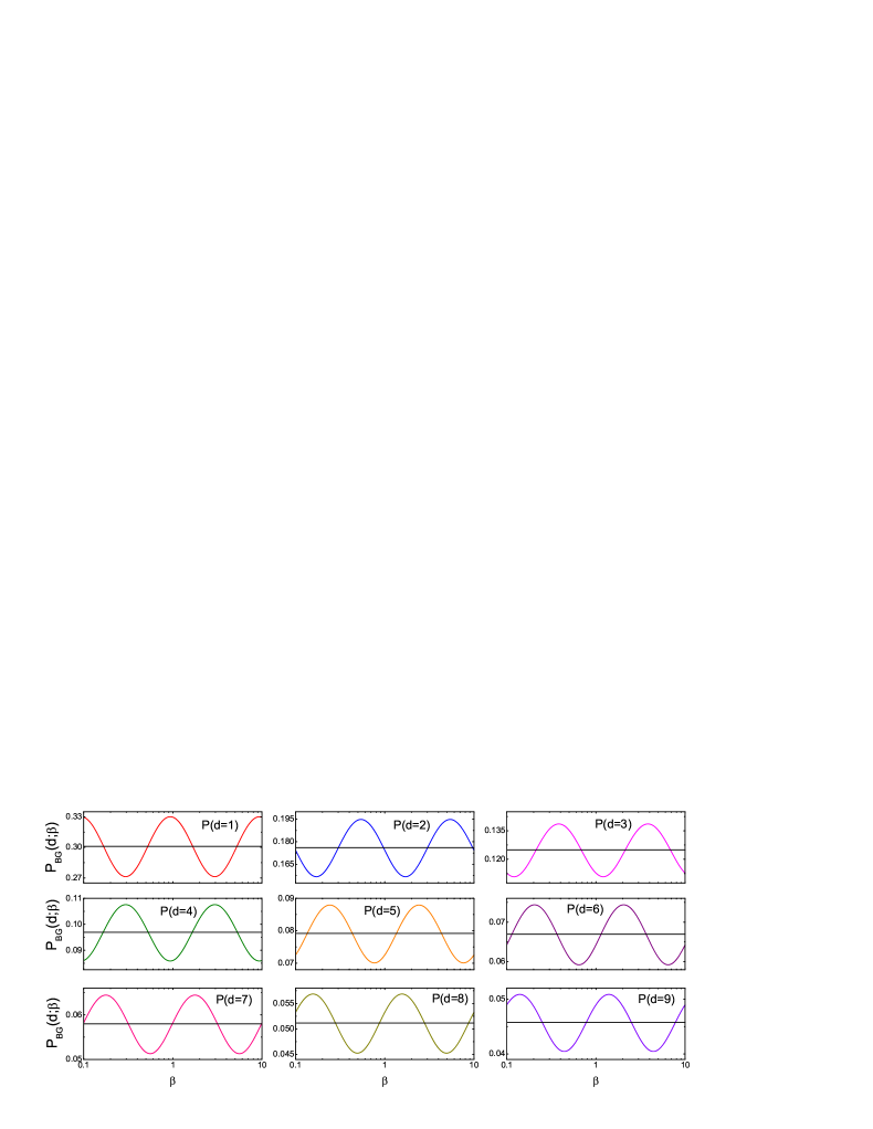
Figure 1: The comparisons of the first digit distributions for BG distribution and Benford’s law via the inverse of temperature $\beta=1/kT$, where $k$ is the Boltzmann constant. The horizontal line in each panel presents the value predicted by Benford’s law (also see Figure 1 in Ref. [35]).

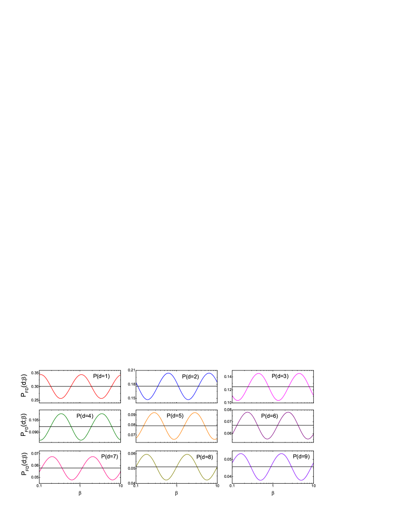
Figure 2: The comparisons of the first digit distributions for FD distribution and Benford’s law via the inverse of temperature $\beta=1/kT$, where $k$ is the Boltzmann constant. The horizontal line in each panel presents the value predicted by Benford’s law.

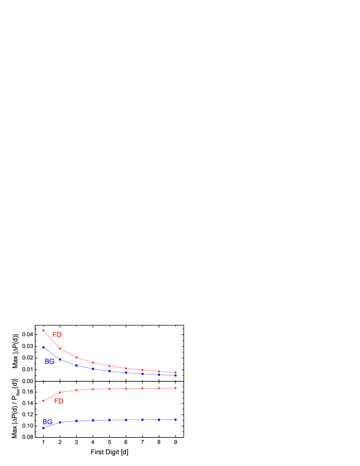
Figure 3: Upper panel: The maximum deviation of the first digit distributions from Benford’s law for the BG distribution (squared) and the FD distribution (star-shaped); Lower panel: the maximum relative deviation of the first digit distributions from Benford’s law for the BG distribution (squared) and the FD distribution (star-shaped).

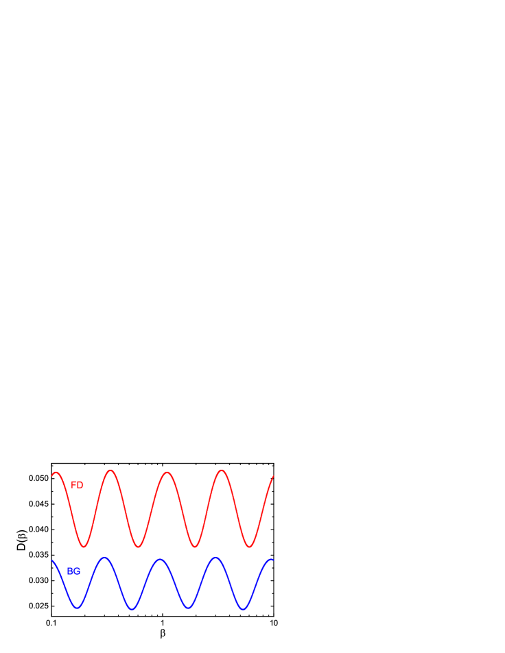
Figure 4: The distances of the first digit distributions of BG and FD statistics from Benford’s law versus the inverse temperature $\beta=1/kT$.

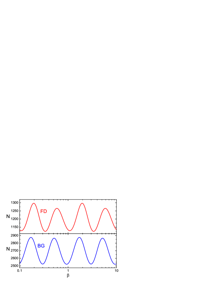
Figure 5: The minimum sizes of samples required to distinguish the first digit distributions of BG (lower panel) and FD (upper panel) statistics from Benford’s law versus the inverse temperature $\beta=1/kT$, under the confidence level 95%.

References

- [1] S. Newcomb, Am. J. Math. 4 (1881) 39-40.
- [2] F. Benford, Proc. Am. Phil. Soc. 78 (1938) 551-572.
- [3] J. Burke, E. Kincanon, Am. J. Phys. 59 (1991) 952-952.
- [4] E. Ley, Am. Stat. 50 (1996) 311-313.
- [5] J. Torres, S. Fernández, A. Gamero, A. Sola, Eur. J. Phys. 28 (2007) L17-L25.
- [6] L.M. Leemis, B.W. Schmeiser, D.L. Evans, Am. Stat. 54 (2000) 236-241.
- [7] L. Shao, B.-Q. Ma, Mod. Phys. Lett. A 24 (2009) 3275-3282 [arXiv:1004.3077].
- [8] L. Shao, B.-Q. Ma, Astropart. Phys. 33 (2010) 255-262.
- [9] C.R. Tolle, J.L. Budzien, R.A. LaViolette, Chaos 10 (2000) 331-336.
- [10] A. Berger, L.A. Bunimovich, T.P. Hill, T. Am. Math. Soc. 357 (2005) 197-219.
- [11] A. Berger, Discrete Cont. Dyn. S. 13 (2005) 219-237.
- [12] M.J. Nigrini, J. Am. Tax. Assoc. 18 (1996) 72-91.
- [13] M.J. Nigrini, L.J. Mittermaier, Auditing 16 (1997) 52-67.
- [14] A.M. Rose, J.M. Rose, Journal of Accountancy 196 (2003) 58-60.
- [15] C.L. Geyer, P.P. Williamson, Commun. Stat.-Simul. C. 33 (2004) 229-246.
- [16] J.L. Barlow, E.H. Bareiss, Computing 34 (1985) 325-347.
- [17] P. Schatte, J. Inform. Process. Cybern. EIK 24 (1988) 443-455.
- [18] A. Berger, T.P. Hill, Am. Math. Mon. 114 (2007) 588-601.
- [19] R.A. Raimi, Am. Math. Mon. 76 (1969) 342-348.
- [20] R.A. Raimi, Sci. Am. 221 (1969) 109-119.
- [21] R.A. Raimi, Am. Math. Mon. 83 (1976) 521-538.
- [22] R.A. Raimi, Proc. Am. Phil. Soc. 129 (1985) 211-219.
- [23] T.P. Hill, Am. Math. Mon. 102 (1995) 322-327.
- [24] T.P. Hill, P. Am. Math. Soc. 123 (1995) 887-895.
- [25] T.P. Hill, Stat. Sci. 10 (1995) 354-363.
- [26] T.P. Hill, Am. Sci. 86 (1998) 358-363.
- [27] T.P. Hill, K. Schürger, J. Stoch. Proc. Appl. 115 (2005) 1723-1743.
- [28] A. Berger, T.P. Hill, K.E. Morrison, J. Theor. Probab. 21 (2008) 97-117.
- [29] R.S. Pinkham, Ann. Math. Stat. 32 (1961) 1223-1230, though there contains a fundamental error in this proof [21].
- [30] J.J. Shen, Y.M. Zhao, Sci. China Ser. G 52 (2009) 1477-1481.
- [31] D.S. Lemons, Am. J. Phys. 54 (1986) 816-817.
- [32] L. Pietronero, E. Tosatti, V. Tosatti, A. Vespignani, Physica A 293 (2001) 297-304.
- [33] L. Boltzmann, Wien. Ber. 76 (1877) 373-435.
- [34] J.W. Gibbs, Elementary Principles in Statistical Mechanics, Dover, New York, 1901.
- [35] H.-A. Engel, C. Leuenberger, Stat. Probabil. Lett. 63 (2003) 361-365.
- [36] B. Buck, A.C. Merchant, S.M. Perez, Eur. J. Phys. 14 (1993) 59-63.
- [37] D. Ni, Z. Ren, Eur. Phys. J. A 38 (2008) 251-255.
- [38] J.C. Pain, Phys. Rev. E 77 (2008) 012102.
- [39] E. Fermi, Rend. Lincei 3 (1926) 145-149.
- [40] P.A.M. Dirac, Proc. R. Soc. A 112 (1926) 661-677.
- [41] S.N. Bose, Z. Phys. 26 (1924) 178-181.
- [42] A. Einstein, Sitz. Ber. Preuss. Akad. Wiss. 22 (1924) 261-267.
- [43] C. Beck, E.G.D. Cohen, Physica A 322 (2003) 267-275.
- [44] P. Diaconis, D. Freedman, J. Am. Stat. Assoc. 74 (1979) 359-364.