Tricolored Lattice Gauge Theory with Randomness:
Fault-Tolerance in Topological Color Codes

Abstract

We compute the error threshold of color codes—a class of topological quantum codes that allow a direct implementation of quantum Clifford gates—when both qubit and measurement errors are present. By mapping the problem onto a statistical-mechanical three-dimensional disordered Ising lattice gauge theory, we estimate via large-scale Monte Carlo simulations that color codes are stable against 4.8(2)% errors. Furthermore, by evaluating the skewness of the Wilson loop distributions, we introduce a very sensitive probe to locate first-order phase transitions in lattice gauge theories.

1 Introduction

The study of quantum error correction in topological stabilizer codes [1] burgeoned a magnificent synergy between quantum computation and statistical-mechanical systems with disorder [2]. Quantum error-correction [3, 4] is a method to preserve quantum information from decoherence by actively detecting and counteracting errors using redundancy. In topological codes, these error-detecting operations are local and one can relate the stability of a topological quantum memory to an ordered phase in a classical statistical model [2]. The error threshold—a figure of merit that describes the stability of a system against local errors and up to which error correction is feasible—can be identified with the critical point at which the ordered phase of the underlying statistical mechanical system is lost due to the influence of quenched disorder.

In most studies, it is assumed that the error-correction procedure is free of errors. However, error-correction is achieved by means of applying a set of quantum gates and this procedure can be flawed as well, leading to the concept of fault-tolerance [5, 6, 7]. In a topological quantum memory, the information is encoded in global degrees of freedom [2] and preserved by repeatedly performing local measurements to keep track of and correct for errors. To understand the error resilience, it is convenient to adopt a phenomenological description of errors [2]. Errors are assumed to be nonsystematic and uncorrelated both in space and in time. Therefore, the error modeling process is parametrized in terms of two error rates: the qubit error rate $p$ and the measurement error rate $q$. At each complete step in the syndrome measurement process, each physical qubit in the memory can suffer an error with an independent probability $p$ and each measurement outcome can be incorrect with probability $q$. For the case of toric codes [1], which were the first example of topological codes, error correction ($q=0$) can be studied via the two-dimensional (2D) random-bond Ising model [8, 9]. Including faulty measurements ($q>0$), the error process is mapped onto a 3D random-plaquette gauge model [2, 10].

\psfrag{a}{\large a}\psfrag{b}{\large b}\psfrag{c}{\large c}\psfrag{d}{\large d}\psfrag{e}{\large e}\psfrag{f}{\large f}\psfrag{g}{\large g}\psfrag{H}{\large$\mathcal{H}$}\psfrag{T}{\large$\mathcal{T}$}\includegraphics[width=390.25534pt]{lattice.eps}

Figure 1: Left: Lattice representing the error history. Right: Derived lattice for the lattice gauge theory model. Time corresponds to the vertical axis. The vertices of the $\mathcal{T}$ layers and the hexagons of the $\mathcal{H}$ layers are three-colored. (a,b) Elementary equivalences between error histories. (c,d) Hamiltonian terms (five-body and planar hexagons). (e) Flipping the encircled spins is a gauge symmetry. (f) Horizontal Wilson loop. In this work we study elemental loops encircling one hexagonal plaquette. (g) Excitations are colored fluxes.

More recently [11, 12] other approaches to topological quantum error correction have been introduced. For example, topological color codes (TCC) are a class of topological codes that allow the transversal implementation of the Clifford group of quantum gates [11, 12]. Remarkably, these enhanced computational capabilities for quantum distillation, teleportation, dense coding, etc. are possible while preserving a high error threshold [13] (in comparison to the Kitaev model [1]). This result has been obtained numerically after mapping the error correction ($q=0$) for TCCs onto a random three-body Ising model on a triangular lattice [13]; later confirmed by other numerical methods [14, 15, 16]. It is, however, unclear if quantum computations on TCCs can be performed reliably in the presence of faulty measurements ($q\neq 0$). Here we address this problem by simulating a complex disordered lattice gauge theory (LGT) [17] – a task that required the introduction of novel tools to probe for an ordered phase. Our main results are:

$\Box$ A complete study of error correction in TCCs. We find that, for equal error qubit flip and measurement error rates $p=q$, the error threshold is $p_{c}=4.8(2)\%$.

$\Box$ A novel Abelian lattice gauge theory with gauge group ${\mathbb{Z}}_{2}\times{\mathbb{Z}}_{2}$ and a peculiar lattice and gauge structure that departs from the standard formulations of Wegner [18] and Wilson [19], see Fig. 1. We refer to it as a tricolored LGT. Its structure reflects the error history in color codes, rather than the discretization of a continuous gauge theory.

$\Box$ A novel approach to pinpoint first-order phase transitions in LGTs with disorder using the skewness of the average over Wilson loop operators.

2 Error Correction with Faulty Measurements

To construct a topological color code, we consider a hexagonal arrangement of the physical qubits on a 2D surface, such that the dual lattice has a regular triangular form with 3-colorable vertices (i.e., the vertices can be labeled with three colors such that adjacent vertices have different colors). Note that each triangle $\triangle$ of the dual lattice $\mathcal{T}$ (see Fig. 1) corresponds to a physical qubit in the initial arrangement. We now attach to each vertex $v$ two Pauli operators,

$$X_{v}:=\otimes_{\triangle\ni v}X_{\triangle},\quad Z_{v}:=\otimes_{\triangle\ni v}Z_{\triangle}\,,$$ (1)

which act on the physical qubits associated with the six triangles adjacent to $v$. These are called check operators because encoded states $|\psi\rangle$ satisfy $X_{v}|\psi\rangle=Z_{v}|\psi\rangle=|\psi\rangle$. Such states exist because the group generated by check operators, called stabilizer group, does not contain $-\mathbf{1}$, so that in particular check operators commute with each other. The dimension of the encoded subspace depends only on the topology of the surface where the code lives, something that is true in part due to the colorability properties of the lattice. For example, a regular lattice with periodic boundary conditions has the topology of a torus and encodes two logical qubits [11]. As in any topological code, a main feature is that local operators cannot distinguish different encoded states.

To keep track of errors, check operators are measured repeatedly over time, allowing for the detection of local inconsistencies with the code. Error correction amounts to guessing the correct error history $E$ among those that are compatible with the measurement outcomes. Indeed, many error histories have an equivalent effect, and thus the ideal strategy is to compute which equivalence class $\bar{E}$ happened with the highest probability $P(\bar{E})$. Therefore, error correction is highly successful when for typical errors there is a class that dominates over the others. Color codes, being topological, have an error threshold below which the success probability approaches unity in the limit of large codes.

Because color codes are Calderbank-Shor-Steane (CSS) codes [20, 21], $X$ (bit-flip) and $Z$ (phase-flip) errors can be corrected separately. In doing so one ignores any correlations between bit-flip and phase-flip errors, something that can only make error correction worse. Then, for simplicity, we assume an error model where bit-flip and phase-flip errors are uncorrelated. Before each round of measurements each qubit is subject to the channel

$$\rho\longrightarrow(1-p)^{2}\rho+p(1-p)(X\rho X+Z\rho Z)+p^{2}Y\rho Y,$$ (2)

where $\rho$ represents the state of a single qubit and $p$ is both the probability for a bit-flip error to occur and the probability for a phase-flip error to occur. As for the measurement outcomes of check operators, each of them is wrong with independent probability $q$.

We focus on bit-flip errors, which change the eigenvalue of all adjacent $Z_{v}$ check operators; $Z$ errors are analogous. Identifying time with the vertical direction, we form a lattice of stacked triangle layers, one per measurement round, with vertical connections (see Fig. 1, left). Error histories are represented as collections of triangles representing bit-flip errors and vertical links that represent measurement errors. If an error history $E$ is composed by a total of $b$ bit-flip errors and $m$ wrong measurement outcomes, its probability is

$$P(E)=(1-p)^{N-b}(1-q)^{M-m}p^{b}q^{m}\propto\left(\frac{p}{1-p}\right)^{b}\left(\frac{q}{1-q}\right)^{m}$$ (3)

where $N$ is the total number of qubits and $M$ the total number of check operators.

Following Ref. [2], we classify error histories $E$ in equivalence classes $\bar{E}$. Whenever two error histories $E$ and $E^{\prime}$ belong to the same class and an error $E$ has happened, the error correction is still successful even if we wrongly correct according to $E^{\prime}$. The equivalence relation can be constructed from two different kinds of elementary equivalences. First, if $S$ is the set of triangles meeting at a given vertex $v$ [Fig. 1 (a)] and the histories $E$ and $E^{\prime}$ differ exactly on the elements of $S$, then they are equivalent because the local operator $X_{v}$ has no effect on encoded states. In particular, if $P$ is a Pauli operator representing an error history—including $X$ and $Z$ errors—and $\rho$ an encoded state, then

$$X_{v}P\rho P^{\dagger}X_{v}=PX_{v}\rho X_{v}P^{\dagger}=P\rho P^{\dagger}.$$ (4)

We say that these elementary equivalences are of type I. Second, suppose that $S$ is now the set including two triangles, one on top of the other, and the vertical links connecting them [Fig. 1 (b)]. Then if the histories $E$ and $E^{\prime}$ differ exactly on the elements of $S$, they are equivalent because two unnoticed subsequent bit-flips on the same qubit are irrelevant. We say that these elementary equivalences are of type II.

3 Tricolored lattice gauge theory with randomness

As in Ref. [2], the first goal is to express the probabilities of error classes in terms of the partition function of a suitable statistical model. Our goal is to obtain

$$P(\bar{E}):=\sum_{E\in\bar{E}}P(E)\propto Z_{E}(T):=\sum_{\sigma}e^{-\beta H_{E}(\sigma)}$$ (5)

for a suitably parametrized Hamiltonian $H_{E}$. We start by attaching classical spins $\sigma=\pm 1$ to the elementary equivalences between error histories discussed above, both of type I and II. This produces a new lattice [see Fig. 1 (right)] with honeycomb layers $\mathcal{H}$ sandwiched between triangular layers $\mathcal{T}$. Spins on the $\mathcal{T}$-layers [$\mathcal{H}$-layers] correspond to equivalences of type I [type II] while negative interaction constants correspond to errors. There are six-body interactions which stem from measurement errors (vertical links in the previous lattice) that involve the vertices of a given hexagon at a $\mathcal{H}$ layer, see Fig. 1(d). There are also five-body interactions due to bit-flip errors and thus related to triangles in ${\cal T}$-layers: they involve the three vertices of the triangle plus the two $\mathcal{H}$-vertices directly above and below the triangle, see Fig. 1(c). We use the symbol $\textstyle\triangle$ $\textstyle\cdot$ to denote such sets of five vertices. The Hamiltonian of interest is

$$H_{\gamma}(\sigma)=-J\sum_{\mathchoice{\leavevmode\vtop{\halign{\hfil$\displaystyle#$\hfil\cr\triangle\cr\cdot\crcr}}}{\leavevmode\vtop{\halign{\hfil$\textstyle#$\hfil\cr\triangle\cr\cdot\crcr}}}{\leavevmode\vtop{\halign{\hfil$\scriptstyle#$\hfil\cr\triangle\cr\cdot\crcr}}}{\leavevmode\vtop{\halign{\hfil$\scriptscriptstyle#$\hfil\cr\triangle\cr\cdot\crcr}}}}\gamma_{\mathchoice{\leavevmode\vtop{\halign{\hfil$\displaystyle#$\hfil\cr\triangle\cr\cdot\crcr}}}{\leavevmode\vtop{\halign{\hfil$\textstyle#$\hfil\cr\triangle\cr\cdot\crcr}}}{\leavevmode\vtop{\halign{\hfil$\scriptstyle#$\hfil\cr\triangle\cr\cdot\crcr}}}{\leavevmode\vtop{\halign{\hfil$\scriptscriptstyle#$\hfil\cr\triangle\cr\cdot\crcr}}}}\prod_{j\in\mathchoice{\leavevmode\vtop{\halign{\hfil$\displaystyle#$\hfil\cr\triangle\cr\cdot\crcr}}}{\leavevmode\vtop{\halign{\hfil$\textstyle#$\hfil\cr\triangle\cr\cdot\crcr}}}{\leavevmode\vtop{\halign{\hfil$\scriptstyle#$\hfil\cr\triangle\cr\cdot\crcr}}}{\leavevmode\vtop{\halign{\hfil$\scriptscriptstyle#$\hfil\cr\triangle\cr\cdot\crcr}}}}\sigma_{j}-K\sum_{\hexagon}\gamma_{\hexagon}\prod_{k\in\hexagon}\sigma_{k}\,,$$ (6)

where $J>0$ and $K>0$, $\gamma_{\mathchoice{\leavevmode\vtop{\halign{\hfil$\displaystyle#$\hfil\cr\triangle\cr\cdot\crcr}}}{\leavevmode\vtop{\halign{\hfil$\textstyle#$\hfil\cr\triangle\cr\cdot\crcr}}}{\leavevmode\vtop{\halign{\hfil$\scriptstyle#$\hfil\cr\triangle\cr\cdot\crcr}}}{\leavevmode\vtop{\halign{\hfil$\scriptscriptstyle#$\hfil\cr\triangle\cr\cdot\crcr}}}},\gamma_{\hexagon}=\pm 1$ and $j$ [$k$] runs over the vertices of each $\textstyle\triangle$ $\textstyle\cdot$ [$\hexagon$]. Given an error history $E$, let $\gamma^{E}$ be such that $\gamma^{E}_{\mathchoice{\leavevmode\vtop{\halign{\hfil$\displaystyle#$\hfil\cr\triangle\cr\cdot\crcr}}}{\leavevmode\vtop{\halign{\hfil$\textstyle#$\hfil\cr\triangle\cr\cdot\crcr}}}{\leavevmode\vtop{\halign{\hfil$\scriptstyle#$\hfil\cr\triangle\cr\cdot\crcr}}}{\leavevmode\vtop{\halign{\hfil$\scriptscriptstyle#$\hfil\cr\triangle\cr\cdot\crcr}}}}=-1$ when the triangle in $\textstyle\triangle$ $\textstyle\cdot$ belongs to $E$, and similarly for hexagons $\hexagon$ and their dual vertical links. Also, let $\sigma_{0}$ represent the state with all spins in the +1 state. Then

$$P(E)\propto e^{-\beta H_{\gamma^{E}}(\sigma_{0})}$$ (7)

if the inverse temperature $\beta=1/T$ as well as $J$ and $K$ satisfy the conditions

$$e^{-2\beta J}=p/(1-p)\qquad\mathrm{and}\qquad e^{-2\beta K}=q/(1-q)\,.$$ (8)

Moreover, if two spin configurations $\sigma_{1}$ and $\sigma_{2}$ only differ by the sign of a single spin, and two error histories $E_{1}$ and $E_{2}$ are equivalent up to the corresponding elementary equivalence, then

$$H_{\gamma^{E_{1}}}(\sigma_{1})=H_{\gamma^{E_{2}}}(\sigma_{2}).$$ (9)

Putting together Eqs. (7) and (9) we obtain the desired result

$$P(\bar{E})\propto Z_{\gamma^{E}}(\beta J):=\sum_{\sigma}e^{-\beta H_{\gamma^{E}}(\sigma)}.$$ (10)

Following Ref. [2], the next step is to consider a model with a Hamiltonian [Eq. (6)] where the parameters $\gamma$ are quenched variables, with $p$ and $q$ dictating the probability distribution of the $\gamma$’s such that $P(\gamma^{E}):=P(E)$. That is, each $\textstyle\triangle$ $\textstyle\cdot$ [$\hexagon$] has negative sign with probability $p$ [$q$]. The resulting system has four parameters, $\beta J$, $\beta K$, $p$ and $q$. The connection between error correction in color codes and this statistical model happens along the sheet described by the Nishimori conditions, Eqs. (8). In that sheet, order in the statistical model corresponds to errors being correctable [2]. For the sake of simplicity, we set $p=q$, assuming the same fault rate for qubit and measurement errors. In that case it is enough to consider a statistical model with $K=J$, so that it has only two parameters, namely $\beta J$ and $p$. The critical $p$ along the Nishimori line

$$e^{-2\beta J}=p/(1-p)$$ (11)

then gives the fault-tolerance threshold $p_{c}$ for color codes.

4 Gauge Symmetry

The Hamiltonian in Eq. (6) has a local symmetry per hexagon $\hexagon$: flipping its spins and those above and below its center [Fig. 1(e)] leaves the energy invariant. This is a ${\mathbb{Z}}_{2}\times{\mathbb{Z}}_{2}$ gauge symmetry, as the construction of suitable Wilson loops demonstrates. Let us label $\mathcal{H}$-hexagons according to the coloring of the $\mathcal{T}$-vertices. Wilson loops come also in three colors. For example, a blue horizontal loop is the product of green and blue hexagonal terms [Fig. 1(f)]. Since there are two independent Wilson loops for a given surface with a single boundary, there are four possible flux values going through it. Moreover, the total flux through two regions is trivial if both have the same flux, showing that the gauge is ${\mathbb{Z}}_{2}\times{\mathbb{Z}}_{2}$. Indeed, excitations can be regarded as colored fluxes. First, depict an excited hexagon as a vertical flux of the corresponding color. Second, depict an excited triangle as the three merging fluxes (one of each color). Using this convention, excitations take the form of closed colored strings with branching points where three different colors meet [Fig. 1(g)].

5 Simulation Details

The study of the partition function [Eq. (6)] constitutes a considerable numerical challenge. To compute the error threshold including bit-flip and measurement errors, we need to compute the $p\,$–$q\,$–$T_{c}$ phase diagram of the model. The special case of equal error rates ($p=q$) studied here provides a useful guidance, however, 23.4 CPU years ($6.4\cdot 10^{15}$ operations on Brutus) were needed to obtain the results in Fig. 5.

Table 1: Simulation parameters: $L$ is the layer size, $M$ is the number of layers, $N_{\rm sa}$ is the number of disorder samples, $t_{\rm eq}=2^{b}$ is the number of equilibration sweeps, $T_{\rm min}$ [$T_{\rm max}$] is the lowest [highest] temperature, and $N_{\rm T}$ the number of temperatures used.

$p$	$L$	$M$	$N_{\rm sa}$	$b$	$T_{\rm min}$	$T_{\rm max}$	$N_{\rm T}$
$0.00$	$6$, $9$	$6$, $8$	$1600$	$15$	$1.20$	$2.00$	$64$
$0.00$	$12$	$12$	$800$	$15$	$1.20$	$2.00$	$64$
$0.00$	$15$	$14$	$400$	$17$	$1.20$	$2.00$	$64$
$0.02$	$6$, $9$	$6$, $8$	$1600$	$16$	$0.90$	$1.80$	$52$
$0.02$	$12$	$12$	$800$	$17$	$0.90$	$1.80$	$52$
$0.02$	$15$	$14$	$400$	$19$	$0.90$	$1.80$	$52$
$0.03$–$0.039$	$6$, $9$	$6$, $8$	$1600$	$17$	$0.70$	$1.40$	$52$
$0.03$–$0.039$	$12$	$12$	$800$	$19$	$0.70$	$1.40$	$52$
$0.03$–$0.039$	$15$	$14$	$400$	$21$	$0.70$	$1.40$	$52$
$0.04$–$0.060$	$6$, $9$	$6$, $8$	$1600$	$18$	$0.50$	$1.20$	$52$
$0.04$–$0.060$	$12$	$12$	$800$	$20$	$0.50$	$1.20$	$52$
$0.04$–$0.060$	$15$	$14$	$400$	$22$	$0.50$	$1.20$	$52$

Because the model is a LGT the natural (gauge invariant) order parameter is the Wilson loop. Due to the presence of disorder and the complexity of the lattice, a clean scaling analysis using the area/perimeter laws [10] is imprecise because large Wilson loops show strong corrections to scaling. Instead, we investigate in detail the smallest horizontal loops in the system,

$$W_{\hexagon}:=\prod_{k\in\hexagon}\sigma_{k},$$ (12)

which correspond to single hexagon plaquettes $\hexagon$ and record their average value over all loops in the system, i.e.,

$$w=\frac{1}{N_{\hexagon}}\sum_{\hexagon}W_{\hexagon},$$ (13)

suitably averaged over Monte Carlo time and disorder. Without disorder ($p=0$) this order parameter shows a clear signal of a transition. However the detection of the transition temperature $T_{c}$ becomes increasingly difficult when a finite error probability ($p>0$) is introduced. Therefore, we also study the whole distribution $f(w)$. For a first-order phase transition we expect a characteristic double-peak structure to emerge near the transition. To better pinpoint the transition, we introduce a derived order parameter $\zeta$ related to the skewness of the distribution

$$\zeta(\tilde{w})=\left[\left\langle\tilde{w}^{3}\right\rangle_{\mbox{\scriptsize{T}}}\right]_{\mbox{\scriptsize{av}}}/\left[\left\langle\tilde{w}^{2}\right\rangle_{\mbox{\scriptsize{T}}}\right]_{\mbox{\scriptsize{av}}}^{3/2}\,,$$ (14)

where $\tilde{w}=w-\left[\left\langle w\right\rangle_{\mbox{\scriptsize{T}}}\right]_{\mbox{\scriptsize{av}}}$, $\left\langle\cdots\right\rangle_{\mbox{\scriptsize{T}}}$ denotes a thermal average and $\left[\cdots\right]_{\mbox{\scriptsize{av}}}$ represents an average over the disorder. The skewness of a symmetric function is zero and becomes positive (negative) when the function is slanted to the left (right). Therefore we can identify the point where $\zeta$ crosses the horizontal axis with an equally-weighted double peak structure in $f(w)$, i.e., $\zeta(T=T_{c})=0$. We have compared these results to the peaks in the specific heat as well as a Maxwell construction and find perfect agreement. To compute the $p\,$–$T_{c}$ phase diagram, we fix the value of the error rate $p$ and vary the temperature $T$ until we detect a Higgs-to-confining transition for $T=T_{c}$. $T_{c}(p)$ is then the critical line separating both phases. The error threshold $p_{c}$ is given by the crossing point between $T_{c}(p)$ and the Nishimori line [22].

The term “Higgs-to-confining” refers to the transition from one gapped phase to another in a LGT. These gapped phases are characterized by non-vanishing closed string correlators, the Wilson loops, and can be distinguished by investigating the perimeter and area laws, respectively. The Higgs phase corresponds to a perimeter law for the Wilson loop correlator, regardless of whether an explicit Higgs field is present in the theory. The rationale is that static matter sources, when introduced in the Higgs phase, will become unbounded, i.e., deconfined, as opposed to the confinement which occurs in the phase with an area law. Therefore, here the Higgs phase refers to the (magnetically) ordered phase, while the confined phase corresponds to the disordered phase found for larger values of $p$ and $T$.

It has been previously shown [2], that the error threshold is given by the crossing point of the Nishimori line with this phase boundary. We recall that the Nishimori line $T=T(p)$ is the locus describing a quantum computer in the presence of external noise, while the rest of the phase diagram is merely introduced as an auxiliary tool to locate the multicritical point. Note that on the Nishimori line, the effects of thermal fluctuations and quenched randomness are in balance. For weak disorder $p$ and low temperatures $T$, the system is in a magnetically ordered Higgs phase. In terms of the color code, this indicates that all likely error histories for a given error syndrome are topologically equivalent and error recovery is achievable. However, at a critical disorder value $p_{c}$ (and a corresponding temperature determined by Nishimori’s relation), magnetic flux tubes condense and the system enters the magnetically disordered confinement phase. In this case, magnetic disorder means that the error syndrome cannot point to likely error patterns belonging to a unique topological class; therefore the topologically encoded information is vulnerable to damage.

For the simulations we study systems of size $L^{2}\times M$ with $M$ along the vertical direction. Periodic boundary conditions are applied to reduce finite-size effects. The colorability and stacking of the layers requires that $L$ [$M$] is a multiple of $3$ [$2$]. For the system to be as isotropic as possible, we choose parameter pairs such that $M\in\{L,L-1\}$. Because the numerical complexity of the system increases considerably when $p>0$, we use the parallel tempering Monte Carlo technique [23]. Simulation parameters are listed in Table 1. Equilibration is tested by a logarithmic binning of the data. Once the last three bins agree within statistical error bars, the system is deemed to be in thermal equilibrium.

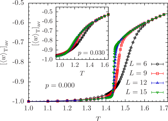
Figure 2: Average Wilson loops for $p=0$ as a function of temperature for different system sizes $L$. For increasing $L$ a sharp drop develops at the transition. The inset shows data for $p=0.03$.

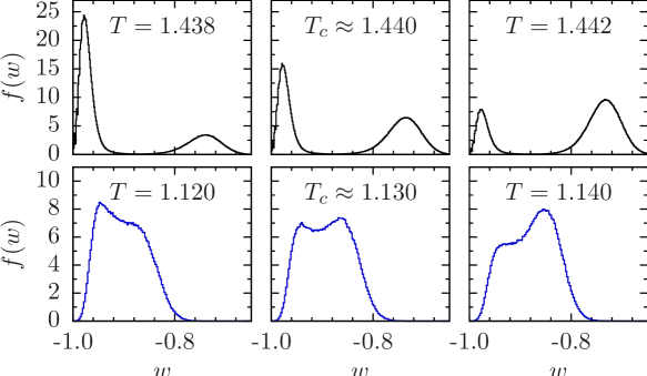
Figure 3: Wilson loop histograms $f(w)$ for systems of size $L=15$ with $p=0$ (top row) and $p=0.03$ (bottom row, blue). The panels show data for temperatures slightly below (left), at (center), and above the transition (right). The double-peak structure is indicative of a first-order transition. For $T\approx T_{c}$ the peaks have equal weight, whereas for $T<T_{c}$ ($T>T_{c}$) it is slanted to the left (right), thus motivating the use of the skewness $\zeta$ (Fig. 4) as an order parameter. All panels have the same horizontal scale.

6 Results

Figure 2 shows the average Wilson loop value as a function of temperature for the pure system ($p=0$) and for an error rate of $p=0.03$ (inset). For the system without disorder, the transition is clearly visible (note that extrapolating to the thermodynamic limit shows that for $p=0$ the transition seems to also be first order. See also Fig. 4). However, when $p>0$ it is difficult to determine the location of the transition. An alternative view is provided by the histogram of Wilson loop values $f(w)$ for different temperatures (Fig. 3). Below $T_{c}$ (left panel), one can observe the development of a shoulder that eventually becomes a second peak. The two peaks have a symmetric weight distribution at the transition temperature (center panel). Above $T_{c}$ the initial peak starts to disappear (right panel) and the distribution slants to the right. This property is mirrored by the skewness of the distribution (Fig. 4). $\zeta(\tilde{w})$ has a positive [negative] peak where the second [first] peak in $f(w)$ develops [disappears], with a zero where the weight distribution is symmetric, i.e., at $T=T_{c}$. We have compared our results using the skewness to the peak position of the specific heat, as well as a Maxwell construction. Not only does the skewness deliver the most precise results, for large disorder ($p\gtrsim 0.03$) it is the only method that reliably shows a sign of a transition, if present. We estimate $T_{c}$ in the thermodynamic limit by plotting the size-dependent crossing point $T_{c}^{*}(N)$ against $1/N$ and applying a linear fit (inset). The full phase diagram is shown in Fig. 5; the crossing between $T_{c}(p)$ and the Nishimori line (thin blue line) determines the error threshold $p_{c}=0.048(2)$. Finally, we would like to note that both vertical and horizontal Wilson loops give $T_{c}$ values that agree within error bars.

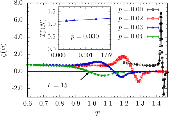
Figure 4: Skewness $\zeta$ for different disorder rates $p$ and $L=15$ as a function of temperature $T$. The crossing points with the horizontal axis (arrow) correspond to where both peaks in the Wilson loop histograms have equal weight, thus signaling the transition. Inset: Example extrapolation of $\zeta[\tilde{w},T=T_{c}^{*}(N)]=0$ to the thermodynamic limit for $p=0.03$.

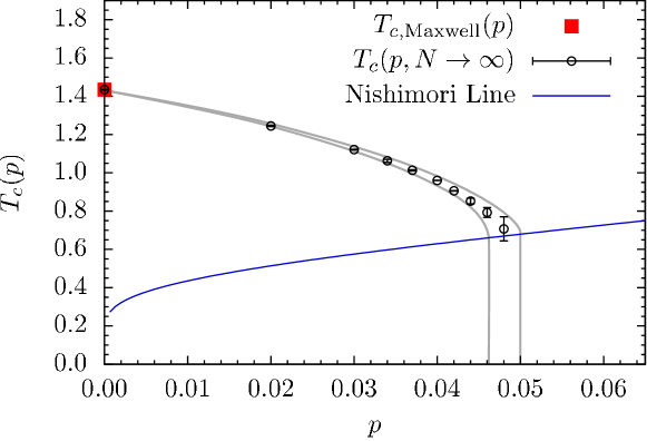
Figure 5: $p\,$–$T_{c}$ phase diagram. For $p>p_{c}=0.048(2)$ errors cannot be recovered. The thin (blue) line represents the Nishimori line. In the regime marked by dashed lines the determination of $T_{c}(p)$ is difficult. The red square is computed using a Maxwell construction of the Wilson loop order parameter and agrees perfectly with the estimate from the skewness.

7 Conclusions

By mapping topological color codes with both qubit and measurement errors onto a classical statistical mechanical model with disorder, we have obtained an Abelian lattice gauge theory with a peculiar lattice and gauge structure. To date, toric codes were the only codes whose complete fault-tolerance properties had been studied. Using Monte Carlo simulations we estimate the error threshold for topological color codes with both bit-flip and measurement errors to be $p_{c}=4.8(2)\%$ (to be compared with $p_{c}\approx 3\%$ for the toric code [10]). To obtain this result we introduce a new approach that uses the skewness of the Wilson loop distribution to pinpoint first-order phase transitions in lattice gauge theories with disorder.

References

References

- [1] A. Yu. Kitaev. Fault-tolerant quantum computation by anyons. Ann. Phys., 303:2, 2003.
- [2] E. Dennis et al. Topological quantum memory. J. Math. Phys., 43:4452, 2002.
- [3] P. W. Shor. Scheme for reducing decoherence in quantum computer memory. Phys. Rev. A, 52:R2493, 1995.
- [4] A. M. Steane. Error Correcting Codes in Quantum Theory. Phys. Rev. Lett., 77:793, 1996.
- [5] P. W. Shor. Fault-tolerant quantum computation. In Proc. of the 37th Symp. on the Foundations of Computer Science, page 56. IEEE Computer Society, 1996.
- [6] E. Knill et al. Threshold Accuracy for Quantum Computation. (arXiv:quant-ph/9610011), 1996.
- [7] D. Aharonov and M. Ben-Or. Fault-tolerant quantum computation with constant error. In Proc. of the 29th annual ACM symp. on Th. of computation., page 188. ACM, 1997.
- [8] S. F. Edwards and P. W. Anderson. Theory of spin glasses. J. Phys. F: Met. Phys., 5:965, 1975.
- [9] H. Nishimori. Statistical Physics of Spin Glasses and Information Processing: An Introduction. Oxford University Press, New York, 2001.
- [10] T. Ohno et al. Phase structure of the random-plaquette gauge model: accuracy threshold for a toric quantum memory. Nucl. Phys. B, 697:462, 2004.
- [11] H. Bombin and M. A. Martin-Delgado. Topological Quantum Distilation. Phys. Rev. Lett., 97:180501, 2006.
- [12] H. Bombin and M. A. Martin-Delgado. Exact topological quantum order in and beyond: Branyons and brane-net condensates. Phys. Rev. B, 75:075103, 2007.
- [13] H. G. Katzgraber et al. Error Threshold for Color Codes and Random 3-Body Ising Models. Phys. Rev. Lett., 103:090501, 2009.
- [14] M. Ohzeki. Accuracy thresholds of topological color codes on the hexagonal and square-octagonal lattices. Phys. Rev. E, 80:011141, 2009.
- [15] D. S. Wang et al. Graphical algorithms and threshold error rates for the 2d colour code. (arXiv:0907.1708), 2009.
- [16] A. Landahl, J. T. Anderson, and P. Rice. in preparation (2009).
- [17] M. Creutz, Quarks, Gluons and Lattices (Cambridge University Press, UK, 1983); C. Itzykson and J.-M. Drouffe, Statistical Field Theory (Cambridge University Press, UK, 1991); I. Montvay and G. Munster, Quantum Fields on a Lattice, (Cambridge Monographs on Mathematical Physics, Cambridge, UK, 1994).
- [18] F. J. Wegner. Duality in Generalized Ising Models and Phase Transitions without Local Order Parameters. J. Math. Phys., 12:2259, 1971.
- [19] K. G. Wilson. Confinement of quarks. Phys. Rev. D, 10:2445, 1974.
- [20] A. R. Calderbank and P. W. Shor. Good quantum error-correcting codes exist. Phys. Rev. A, 54:1098, 1996.
- [21] A. Steane. Multiple-Particle Interference and Quantum Error Correction. Proc. Roy. Soc. Lond. A, 452:2551, 1996.
- [22] H. Nishimori. Internal Energy, Specific Heat and Correlation Function of the Bond-Random Ising Model. Prog. Theor. Phys., 66:1169, 1981.
- [23] K. Hukushima and K. Nemoto. Exchange Monte Carlo method and application to spin glass simulations. J. Phys. Soc. Jpn., 65:1604, 1996.