Observational hints on the Big Bounce

Abstract:

In this paper we study possible observational consequences of the bouncing cosmology. We consider a model where a phase of inflation is preceded by a cosmic bounce. While we consider in this paper only that the bounce is due to loop quantum gravity, most of the results presented here can be applied for different bouncing cosmologies. We concentrate on the scenario where the scalar field, as the result of contraction of the universe, is driven from the bottom of the potential well. The field is amplified, and finally the phase of the standard slow-roll inflation is realized. Such an evolution modifies the standard inflationary spectrum of perturbations by the additional oscillations and damping on the large scales. We extract the parameters of the model from the observations of the cosmic microwave background radiation. In particular, the value of inflaton mass is equal to $m=(2.6\pm 0.6)\cdot 10^{13}$ GeV. In our considerations we base on the seven years of observations made by the WMAP satellite. We propose the new observational consistency check for the phase of slow-roll inflation. We investigate the conditions which have to be fulfilled to make the observations of the Big Bounce effects possible. We translate them to the requirements on the parameters of the model and then put the observational constraints on the model. Based on assumption usually made in loop quantum cosmology, the Barbero-Immirzi parameter was shown to be constrained by $\gamma<1100$ from the cosmological observations. We have compared the Big Bounce model with the standard Big Bang scenario and showed that the present observational data is not informative enough to distinguish these models.

1 Introduction

The observations of the cosmic microwave background (CMB) radiation indicate that the power spectrum of primordial scalar perturbations is in the broad range nearly scale-invariant. Therefore, the spectrum can be written in the power-law form

$$\mathcal{P}_{\text{s}}(k)=A_{\text{s}}\left(\frac{k}{k_{0}}\right)^{n_{\text{s}}-1},$$ (1)

where the spectral index $n_{\text{s}}$ is close to unity. Here, $A_{\text{s}}$ is an amplitude of the scalar perturbations and $k_{0}$ is the so-called pivot number. The case $n_{\text{s}}=1$ corresponds to the scale-invariant Harrison-Zeldovich spectrum. The observed spectrum is almost of this type, namely it is little red-shifted ($n_{\text{s}}\lesssim 1$). In particular, the seven years of observations made by the WMAP satellite [1] indicate that $n_{\text{s}}=0.963\pm 0.012$ (68% CL).

The spectrum in the form discussed above can be explained by the phase of cosmic inflation (see e.g. [2]). This phase can be driven by the self-interacting scalar field, the so-called inflaton field. In the most conservative approach the inflation can be driven by a single massive scalar field. This case will be considered in this paper. In this model, a nearly scale-invariant spectrum spectrum is generated during the slow-roll phase. In a more general case the inflation can be driven with the different potentials. However, the potentials other than massive, lead to the non-Gaussian structure of the cosmic primordial perturbations what can be constrained by the CMB observations [3]. Since the CMB anisotropies do not indicate any non-Gaussian signatures, the massive potential is somehow privileged. However, with the present sensitivity on these kind of effects, some of the other potentials are still allowed. Other models, as multi-field inflation are also possible to be realized. In this paper, we consider the simplest possible realization of the inflation which is given by the single massive scalar field.

The weak point of the slow-roll inflationary scenario is that it requires some special initial conditions. Namely, the field has to start its evolution not from the bottom of potential well but from the position which is far from its center. In the classical model there is no mechanism to drive this field up the potential well. However, it has been recently pointed out [4] that the phase of a quantum bounce can drive the inflaton field up the potential well and set the proper initial conditions for the slow-roll phase. The studies were performed within the loop quantum cosmology (LQC) [5, 6], however the mechanism is generic for all models with the bouncing phase. In the framework of LQC this issue has been studied recently in [4, 7, 8, 9].

In the framework of LQC the classical dynamics of the universe is significantly modified when the energy density approaches the Planck energy density. These effects of the quantum gravitational modification can be introduced as corrections to the classical equations of motion. In particular, the modified Friedmann equation takes the form

$$\left(\frac{1}{a}\frac{da}{dt}\right)^{2}=\frac{8\pi}{3m^{2}_{\text{Pl}}}\rho\left(1-\frac{\rho}{\rho_{\text{c}}}\right),$$ (2)

where the critical energy density is defined as follows

$$\rho_{\text{c}}=\frac{\sqrt{3}}{16\pi^{2}\gamma^{3}}\rho_{\text{Pl}},$$ (3)

where $\rho_{\text{Pl}}:=m^{4}_{\text{Pl}}$ and $m_{\text{Pl}}\approx 1.22\cdot 10^{19}$ GeV is the Planck mass. The above expression (3) is crucial, because it relates the Barbero-Immirzi parameter $\gamma$ with the parameter $\rho_{\text{c}}$, which can be constrained observationally. This is a good example of expressing the phenomenological parameter, as $\rho_{\text{c}}$, in terms of parameters of the underlying theory. In this case the fundamental theory is loop quantum gravity (LQG) with a free parameter $\gamma$.

The value of Barbero-Immirzi parameter is usually fixed from the considerations of the black hole entropy [10]. In particular, the value $\gamma=0.239$ [11] was derived what leads to $\rho_{\text{c}}=0.82\ m^{4}_{\text{Pl}}$. The expression (3) is however not free from ambiguities. In particular, it bases on assumption that the area of the loop in LQC is equal to a gap of the area operator within LQG. This is not necessary true and therefore findings based on expression (3) must be carried with a due care. In general, $\rho_{\text{c}}$ can be treated as a free phenomenological parameter (see e.g. [12, 13, 14]).

2 Inflation in LQC

The global dynamics of the considered model was studied in [15]. It was shown there that the model possesses generic inflationary attractors. However, the particular evolutionary paths can differ. Here we restrict our considerations to the one particular scenario where the energy density is dominated by the kinetic term at the bounce. This condition guarantee that the quantum back-reaction effects can be neglected and equation (2) can be applied. This issue will be discussed in more details at the end of this section.

In the considered evolutionary scenario, we initiate evolution from the contracting phase. The scalar field is initially placed at the bottom of the potential well, what seems to be the realistic and conservative assumption. The initial energy density is therefore contained in the kinetic part only. Because we begin the evolution at the low energy scales, the corresponding time derivative of the field is also small. Another possible choice of initial conditions is given e.g. by saturating the Heisenberg uncertainty relation, then $\pi_{\phi}(t_{0})\phi(t_{0})={\hslash}/2$ at some initial time $t_{0}$.

The field begins its evolution from some tiny quantum fluctuations and starts to oscillate at the bottom of the potential with the time scale of oscillations proportional to $m^{-1}$. The dynamics of the field is governed by the unmodified, standard equation

$$\ddot{\phi}+3H\dot{\phi}+m^{2}\phi=0.$$ (4)

During the contraction, the Hubble factor is negative, and therefore the second term in equation (4) acts as anti-friction. Moreover, while the universe contracts the absolute value of $H$ increases. Therefore as an effect of growing anti-friction, the oscillations are amplified. While approaching the bounce, the field becomes rapidly displaced from the equilibrium state. After that, the standard slow-roll inflation starts. We present the described evolution of the scalar field in Fig. 1.

Figure 1: The shark fin type evolution of the scalar field for $m=10^{-4}m_{\text{Pl}}$. Here $\phi_{\text{max}}\approx 3m_{\text{Pl}}$, what leads to the total number of $e$-foldings $N\approx 56$.

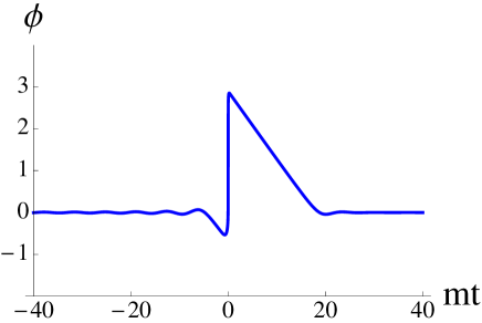
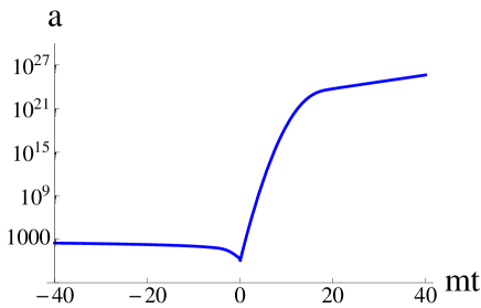
The described evolution corresponds to the shark fin scenario discussed in [9]. During the evolution, the scale factor decreases in the pre-bounce stage. Since in this stage the field behaves effectively as a dust matter, the scale factor $a\propto|t|^{1/3}$. The scale factor reaches its minimal value and then expands almost exponentially, during the slow-roll inflation. While the inflation ends, the scale factor increases as $a\propto|t|^{1/3}$. The numerically computed evolution of the scale factor has been shown in Fig. 2.

Figure 2: Evolution of the scale factor for $m=10^{-4}m_{\text{Pl}}$.

We finish this section with some remarks on the quantum back-reaction effects. These effects become significant when the evolution of the higher moments influences behavior of the mean values of the quantum operators. In the free field case, the evolution of the mean values decouples from the evolution of the higher moments (for detailed discussion of this issue we refer to [16]). The back-reaction effects appear however in the presence of the potential of the scalar field and can significantly modify the effective dynamic. In particular, equation (2) holds only when the quantum back-reaction effects can be neglected. Otherwise this equation can be generalized to [17]

$$\left(\frac{1}{a}\frac{da}{dt}\right)^{2}=\frac{8\pi}{3m^{2}_{\text{Pl}}}\left[\rho\left(1-\frac{\rho_{Q}}{\rho_{\text{c}}}\right)\pm\frac{1}{2}\sqrt{1-\frac{\rho_{Q}}{\rho_{\text{c}}}}\eta(\rho-P)+\frac{(\rho-P)^{2}}{2(\rho+P)}\eta^{2}\right],$$ (5)

and the dynamics can be much more complicated that this discussed previously. Here $\eta$ parameterizes strength of the quantum back-reaction effects. In the considered massive field case the energy density and pressure are respectively

$$\rho=\frac{\dot{\phi}^{2}}{2}+\frac{m^{2}\phi^{2}}{2}\ \ \text{and}\ \ P=\frac{\dot{\phi}^{2}}{2}-\frac{m^{2}\phi^{2}}{2}.$$ (6)

When $P=\rho$, the quantum back-reaction effects disappear, equation (5) simplify to (2). This corresponds to the free field case. Therefore, while the energy density is dominated by the kinetic part, the quantum back-reaction effects can be neglected. In Fig. 3 we show an exemplary evolution of the energy density in the considered model. We also present contributions from the kinetic and potential parts.

Figure 3: The solid (black) curve represents the evolution of the total energy density of the scalar field. The dashed (blue) curve represents the contribution from the kinetic part. The dotted (red) curve represents the contribution from the potential part. In the filled region the energy density is dominated by the kinetic part. Here we have assumed $m=10^{-4}m_{\text{Pl}}$.

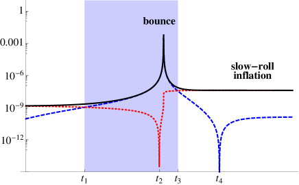
The kinetic term $\frac{\dot{\phi}^{2}}{2}$ dominates the potential part $\frac{m^{2}\phi^{2}}{2}$ in the broad region around the bounce. This is the shadowed region from $t_{1}$ to $t_{3}$ in Fig. 3. Therefore approximation based on (2) holds. For the densities $\rho\ll\rho_{\text{c}}$ the kinetic part can be dominated by the potential part. However, at these densities the quantum effects become unimportant and dynamics can be approximated by the classical equations. Therefore condition $\frac{\dot{\phi}^{2}}{2}\gg\frac{m^{2}\phi^{2}}{2}$ should be fulfilled only in the vicinity of the bounce. If it is not, the quantum back reactions must be taken into account. At time $t_{2}$, the bounce takes place and the energy density reaches its maximal value $\rho_{\text{c}}$. Later, the energy density decreases and holds at approximately constant value. This is the sign that the phase of inflation starts. Precisely, the inflation starts at time $t_{4}$ when the field turns round. At this point, the kinetic term falls to zero since the field stops for a moment. Thereafter, the field makes a slow-roll from the top of the potential well. This part of evolution is almost purely classical and the quantum corrections can be neglected.

3 Observational hints on the slow-roll inflation

Before we proceed to investigate the possible effects due to the bounce, we will firstly discuss the present observational hints regarding the inflation. It is crucial since probing the inflationary phase is more observationally available and give the chance to fix some parameters of the model. We will discuss here what we can already say about the slow-roll inflation model in light of the latest WMAP observations. We also propose the consistency check on the slow-roll inflationary scenario.

The seven years of observations made by the WMAP satellite give the following values of the amplitude and spectral index of the scalar perturbations [1]

$$A_{\text{s}} = 2.441^{+0.088}_{-0.092}\cdot 10^{-9},$$ (7)

$$n_{\text{s}} = 0.963\pm 0.012,$$ (8)

at the pivot scale $k_{0}=0.002\ \text{Mpc}^{-1}$ (see equation (1)). The prediction from the slow-roll is the spectrum of scalar primordial perturbations in the form

$$\mathcal{P}_{\text{s}}(k)=\underbrace{\frac{1}{\pi\epsilon}\left(\frac{H}{m_{\text{Pl}}}\right)^{2}}_{:=S}\left(\frac{k}{aH}\right)^{n_{\text{s}}-1},$$ (9)

as well as the spectrum of the tensor perturbations (gravitational waves) in the form

$$\mathcal{P}_{\text{t}}(k)=\underbrace{\frac{16}{\pi}\left(\frac{H}{m_{\text{Pl}}}\right)^{2}}_{:=T}\left(\frac{k}{aH}\right)^{n_{\text{t}}}.$$ (10)

Expressions for the scalar and tensor spectral indices are respectively

$$n_{\text{s}}=1+2\eta-6\epsilon,$$ (11)

and

$$n_{\text{t}}=-2\epsilon,$$ (12)

where $\epsilon,\eta\ll 1$ are called slow-roll parameters. The $\eta$ and $\epsilon$ are defined in the following way

$$\epsilon \equiv \frac{m^{2}_{\text{Pl}}}{16\pi}\left(\frac{V^{\prime}}{V}\right)^{2}=\frac{m^{2}_{\text{Pl}}}{4\pi}\frac{1}{\phi^{2}},$$ (13)

$$\eta \equiv \frac{m^{2}_{\text{Pl}}}{8\pi}\left(\frac{V^{{}^{\prime\prime}}}{V}\right)=\frac{m^{2}_{\text{Pl}}}{4\pi}\frac{1}{\phi^{2}},$$ (14)

so for the massive inflation field, $\eta=\epsilon$. Based on this and equation (11) we find $\epsilon=(1-n_{\text{s}})/4$. With use of (8), this gives us $\epsilon=0.010\pm 0.003$. Therefore, the slow-roll condition $\epsilon\ll 1$ is indeed fulfilled. Moreover, based on (8), the tensor spectral index is predicted to be

$$n_{\text{t}}=\frac{n_{\text{s}}-1}{2}=-0.019\pm 0.006.$$ (15)

Above we have related observations of the spectral index with the expression predicted from the slow-roll inflation. It was straightforward since both, predicted spectrum (9) and spectrum used in fitting (1) had the same power-law form. However relating the fitted parameter $A_{\text{s}}$ with $S$ requires additional discussion. At the pivot scale $\mathcal{P}_{\text{s}}(k=k_{0})=A_{\text{s}}$. Moreover, we know that the inflationary spectrum at a given mode $k$ is formed when this mode crosses the horizon, namely when $k\simeq aH$. Afterward, the spectrum holds the form fixed at the horizon. Therefore at the given scale $k$, the spectrum is $\mathcal{P}_{\text{s}}(k=aH)=S$. Since $S$ decreases with time, the observed spectrum has the falling tendency (governed by the power law dependence). Based on this, one can relate $\mathcal{P}_{\text{s}}(k=k_{0})=\mathcal{P}_{\text{s}}(k=aH)$, what gives $A_{\text{s}}=S$. Therefore, $A_{\text{s}}$ gives us the value of $S$ at the point when the mode, which is at present equal to $k_{0}$, had crossed the horizon during the inflation. This observation will be crucial for the later considerations.

In order to quantify the contribution from the tensor modes it is convenient to consider the ratio

$$r\equiv\frac{\mathcal{P}_{\text{t}}(k=k_{0})}{\mathcal{P}_{\text{s}}(k=k_{0})}=\frac{T}{S}=16\epsilon=4(1-n_{\text{s}})=0.15\pm 0.05,$$ (16)

where in the last equality we have used the WMAP results (8). This result is consistent with the present constraints on the contribution from the tensor modes

$$r < 2.1\ \text{at}\ 95\%\ \text{CL}\ (\text{WMAP-7},\cite[cite]{[\@@bibref{}{Komatsu:2010fb}{}{}]}),$$ (17)

$$r < 0.73\ \text{at}\ 95\%\ \text{CL}\ (\text{BICEP},\cite[cite]{[\@@bibref{}{Chiang:2009xsa}{}{}]}).$$ (18)

Moreover, the value predicted in (16) is above the observational threshold on detection of the PLANCK satellite [19]. Therefore, if the predictions of the slow-roll inflation are correct, the tensor modes should be observed by the PLANCK mission.

The next parameter that can be computed is the value of the scalar field. Combining (13), (14) and (11) we get

$$\phi_{\text{obs}}=\frac{m_{\text{Pl}}}{\sqrt{\pi(1-n_{\text{s}})}}=2.9\pm 0.5m_{\text{Pl}}.$$ (19)

At this value of field, the observed structures were created . Therefore it can be treated as an lower limit on the maximal displacement of the scalar field. The maximal value of the scalar field is unbounded within the classical theory. However LQC puts the constrain on its value since the energy density is bounded by $\rho_{\text{c}}$. Based on this one find that

$$|\phi|\leq\frac{\sqrt{2\rho_{\text{c}}}}{m}.$$ (20)

The found value of the inflaton field (19) can be translated into the corresponding $e$-folding number

$$N_{\text{obs}}\simeq 2\pi\frac{\phi^{2}_{\text{obs}}}{m^{2}_{\text{Pl}}}=\frac{2}{1-n_{\text{s}}}=54\pm 18.$$ (21)

This is also not the total $e$-folding number for inflation, but only the lower limit on its value. The total $e$-folding number is, in LQC, constrained by

$$N\leq\frac{4\pi\rho_{\text{c}}}{m^{2}_{\text{Pl}}m^{2}},$$ (22)

what bases on (20). Finally one can also derive the mass of inflaton field. Namely

$$m \simeq m_{\text{Pl}}\frac{1}{4}\sqrt{3\pi A_{\text{s}}}(1-n_{\text{s}})$$ (23)

$$= (1.4\pm 0.5)\cdot 10^{-6}m_{\text{Pl}}$$

$$= (2.6\pm 0.6)\cdot 10^{13}\text{GeV}.$$

Therefore, one of the parameters of the model is fixed. The remaining parameter $\rho_{\text{c}}$ is however harder to determinate. We will discuss the present observational constraint on $\rho_{\text{c}}$ in Sec. 6. We stress that it was possible to determinate the value of the parameter $m$ basing only on the observational effects of inflation. It was not necessary to introduce any LQC effects here, because they were negligible during the phase of inflation. In other words, the slow-roll inflation is the classical (and observationally available) part of the considered shark fin scenario.

The usual consistency check of the inflationary models bases on expressing of the tensor-to-scalar $r$ in terms of others (measured) parameters of the model. In case of the slow-roll inflation, we have considered it in equation (16) and we have shown that the derived value of $r$ places within the observational bound. Here, we propose an additional consistency check for inflation. This new consistency relation requires however information about the duration of the reheating phase. Alternatively, the method can be used to put a constraint on the phase of reheating after inflation.

The consistency check base on the fact that the modes created at the particular point of inflation where $\phi=\phi_{\text{obs}}$, correspond to the present pivot scale at which the amplitude of perturbations was computed. These particular modes have the size of horizon when created from the quantum fluctuations. Therefore, at this particular point

$$\lambda_{\text{H}}=2\pi\frac{a}{k}\simeq\frac{1}{H}=\frac{2}{\sqrt{\pi(1-n_{\text{s}})A_{\text{s}}}}=1.2\cdot 10^{5}l_{\text{Pl}}.$$ (24)

In turn, the present pivot scale is equal to

$$\lambda_{0}=\frac{2\pi}{k_{0}}=3.14\cdot 10^{3}\ \text{Mpc}.$$ (25)

Based on this, one can find the total increase of the scale factor from the point at which $\phi=\phi_{\text{obs}}$, till now. We obtain the value

$$\Delta_{\text{tot}}:=\frac{a_{0}}{a_{\text{H}}}=\frac{\lambda_{0}}{\lambda_{\text{H}}}=5\cdot 10^{55}.$$ (26)

There is also another way to compute this quantity. Namely, starting from $\phi=\phi_{\text{obs}}$, the length $\lambda_{\text{H}}$ grows thereafter till the end of inflation, across the reheating, radiation domination phase, matter domination phase until now. It is hard to precisely determinate the increase of the scale factor at this whole evolution. In particular, because we do not know the duration of reheating phase and the duration till the end of inflation was determined with the significant uncertainty. Therefore we can perform only a raw approximation of the total increase of the scale factor.

Let us collect the particular contributions starting from the present and going backward:

• Matter era. The period from recombination till now. $\Delta_{\text{mat}}:=1+z_{\text{dec}}\simeq 10^{3}$

• Radiation era. The period from the end of reheating till the recombination. $\Delta_{\text{rad}}:=\frac{T_{\text{GUT}}}{T_{\text{dec}}}=\frac{10^{14}\ \text{GeV}}{0.2\ \text{eV}}\simeq 5\cdot 10^{23}$

• Reheating (see e.g. [20, 21]). The period when the particles are created from the decaying inflaton field and the universe thermalizes. The corresponding quantity $\Delta_{\text{reh}}$ is model dependent and should be fixed for the particular scenario. For instance, for the instantaneous reheating $\Delta_{\text{reh}}\sim 1$. However, for the considered chaotic inflation the duration of reheating can be longer. We leave detailed considerations to this issue for the further studies, and now let the value of $\Delta_{\text{reh}}$ as a free parameter.

• Inflation. The increase of the scale factor is equal to $\Delta_{\text{inf}}:=e^{N_{\text{obs}}}\simeq 3\cdot 10^{23}$

Based on this, the total increase of the scale factor is equal to

$$\Delta_{\text{tot}}=\Delta_{\text{inf}}\Delta_{\text{reh}}\Delta_{\text{rad}}\Delta_{\text{mat}}.$$ (27)

The left side in equation (27) is determined from (26). Based on the above relation one can e.g. try to determine duration of reheating. Namely, we have

$$\Delta_{\text{reh}}=\frac{\Delta_{\text{tot}}}{\Delta_{\text{inf}}\Delta_{\text{rad}}\Delta_{\text{mat}}}=\frac{5\cdot 10^{55}}{1.5\cdot 10^{51}}\simeq 3\cdot 10^{4}.$$ (28)

On the other hand, in order to use (27) to verify the model of inflation, the duration of reheating must be known from the theory. Then one can define the quantity

$$\theta:=\frac{\Delta_{\text{tot}}}{\Delta_{\text{inf}}\Delta_{\text{reh}}\Delta_{\text{rad}}\Delta_{\text{mat}}}=\frac{\pi^{3/2}\sqrt{(1-n_{\text{s}})A_{\text{s}}}}{k_{0}\exp\left(\frac{2}{1-n_{\text{s}}}\right)\Delta_{\text{reh}}\frac{T_{\text{GUT}}}{T_{\text{dec}}}(1+z_{\text{dec}})}$$ (29)

This is consistency relation for the cosmological model with the slow-roll inflation. The meaningful cosmological should fulfill the condition $\theta\approx 1$. At present, the application of (29) is limited due to the unknown factor $\Delta_{\text{reh}}$. However, it could be possible to determine this value basing on the found value of $m$ and the decay rate of the inflaton field. This issue requires however detailed studies, therefore we leave it to investigate elsewhere.

4 Modified inflationary spectrum and the CMB

As it was shown in Introduction, the spectrum from the slow-roll inflation can be parametrized in the power-law form. However, the prior phase of a bounce should results with modification of this spectrum. The modifications of the primordial scalar spectrum, were investigated in the numerous papers [22, 23, 24]. However, the studies were performed only when the evolution of the scalar modes hold the classical form. Within loop quantum cosmology, not only the dynamics of the background is modified but also the perturbations [25, 26]. In case of the tensor modes (gravitational waves), the form of these modifications was studied in details [27, 28, 29, 30]. Based on this, the spectrum from the shark fin scenario considered has been recently found in [9]. In this paper both quantum corrections to the background as well to the perturbation part were taken into account. The case of the scalar modes is however more problematic. It is because of the issue of quantum anomalies of the algebra of constrains. In case of the so-called inverse-volume corrections, this problem has been resolved [31]. However, in case of the holonomy corrections the anomaly free equations are still not available. Some preliminary attempts to investigate LQC effects on the scalar power spectrum were performed in Ref. [32]. However, the evolution of modes was treated classically and the quantum effects were introduced by the influence on the matter part. Also so attempts to derive holonomy corrected equations on scalar modes were performed in Ref. [33]. However, the authors neglected the issue of the anomaly free algebra of constraint. Therefore derived equations can drive the system out of the surface of constraint and lead to erroneous predictions. Therefore, the systematic analysis of the anomaly freedom in case of the holonomy corrected scalar perturbations remains to be done.

Before the details of modifications of the scalar power spectra will be available, it is advisable to perform the phenomenological analysis of the possible impact of these effects on the CMB spectrum. This issue of impact of the LQC effects on the CMB spectrum was also discussed in Ref. [4, 34, 35]. However, here we perform quantitative analysis in contrast of the much more qualitative discussion in the cited papers. We assume that the scalar power spectrum takes a form

$$\mathcal{P}_{\text{s}}(k) = \Delta(k,k_{*})A_{\text{s}}\left(\frac{k}{k_{0}}\right)^{n_{\text{s}}-1}.$$ (30)

This is, in fact, the standard inflationary spectrum modified by the additional prefactor $\Delta(k,k_{*})$. The bounce-factor $\Delta(k,k_{*})$ can be written as

$$\Delta(k,k_{*})=1-\frac{\sin\left(\frac{3k}{2k_{*}}\right)}{\left(\frac{3k}{2k_{*}}\right)},$$ (31)

which is the simplified form of the expression found in [4]. The $k_{*}$ is a parameter of the model and its interpretation will be discussed later. The factor $\Delta(k,k_{*})$ reflects typical modifications which appear in the bouncing cosmology. In the UV limit, $\lim_{k\rightarrow\infty}\Delta(k,k_{*})=1$, therefore the spectrum (1) is recovered. In turn, in the IR limit, $\lim_{k\rightarrow 0}\Delta(k,k_{*})=0$, and the spectrum is suppressed. This behavior of the power spectrum is typical for the bouncing cosmologies. The two effects of the bounce are transparent: suppression on the low $k$ and the additional oscillations. In Fig. 4 we show function $\Delta$ defined by equation (31). Instead of using the wavenumber $k$ we have translated it to the corresponding length $\lambda=\frac{2\pi}{k}$, respectively $\lambda_{*}=\frac{2\pi}{k_{*}}$.

Figure 4: Plot of function $\Delta$ defined by equation (31) (solid line). The dashed line represents approximation (32).

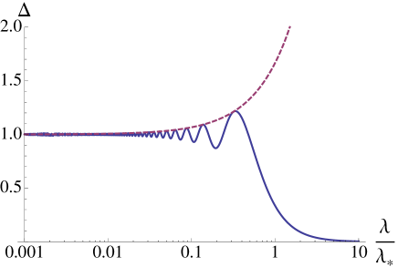
In Fig. 4 we also show the function

$$\Delta(\lambda,\lambda_{*})\approx 1+\frac{2}{3}\frac{\lambda}{\lambda_{*}}.$$ (32)

This function measures the modification due to the oscillations for $\lambda/\lambda_{*}\ll 1$. At $\lambda/\lambda_{*}\approx 1$ the spectrum becomes suppressed. In the bouncing cosmology the length scale $\lambda_{*}$ can be related with the scale of horizon at the beginning of inflation. This issue was discussed in details in [9]. Therefore if the present value of the scale factor is equal $a_{0}=1$ (as used in this paper), we have $k_{*}\simeq a_{i}H_{i}$ where $a_{i}$ is the value of the scale factor at the beginning of inflation and $H_{i}$ is the value of the Hubble factor at the same time. Therefore if $k_{*}$ and $H_{i}$ could be measured, the total increase of the scale factor, from the beginning of inflation till present, can be determined. The value of $k_{*}$ and respectively $\lambda_{*}$ which is a scale of suppression in the spectrum is the crucial observational parameter of the bounce. In this paper we make an attempt of determining this value based on the observations of the CMB.

As mentioned earlier, beside the effect of suppression, also oscillations of the spectrum are predicted within the bouncing cosmologies. This effects is much weaker that suppression, however is present also on the much smaller scales. This is important from the observational point of view. Namely, the length scale $\lambda_{*}=\frac{2\pi}{k_{*}}$ can be much larger than the present size of horizon ($k/k_{*}\ll 1$). Then, the effect of suppression would be inaccessible observationally. However, some oscillations are still present on the sub-horizontal scales. Of course the amplitude of these oscillations decreases while $k/k_{*}\gg 1$. If the scale $\lambda_{*}$ is however not much higher than the size of horizon, the effect of sub-horizontal oscillations could be quite significant. The oscillations in the primordial power spectrum translate into the additional oscillation in the spectrum of the CMB anisotropies (see e.g. [36]). For the small multipoles, this subtle effect can be dominated by the contribution from the cosmic variance. However, for the larger multipoles this effect can dominate. At these scales, improvement of the instrumental resolution are still possible, what gives the chance to, at least, put a stronger constrain on these effects.

In this section we confront the spectrum (30) with observed anisotropies of the cosmic microwave background radiation. We use the seven years of observations made by the WMAP satellite [1]. In the numerical calculations we use the publicly available CAMB code [37] and Markov Chain Monte Carlo (MCMC) package CosmoMC [38] together with the CosmoClust code [39] for computing the Bayesian evidence. The codes were suitably modified to investigate the spectrum (30). In computations, we take the standard cosmological parameters as follows

$$(H_{0},\Omega_{b}h^{2},\Omega_{c}h^{2},\tau)=(70,0.0226,0.112,0.09)$$ (33)

and the pivot scale $k_{0}=0.05\ \text{Mpc}^{-1}$.

In Fig. 5 we show spectrum of the CMB temperature anisotropies obtained based on power spectrum (30).

Figure 5: Spectrum of the CMB anisotropy.

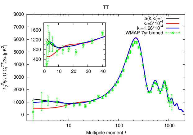
The case $\Delta(k,k_{*})=1\ (k\rightarrow 0)$ corresponds to the classical case with no contribution due to the bounce. The blue line corresponds to the best fit case. In this case, the modulations on the low multipoles are well reproduced. This is due to the oscillations in the primordial power spectrum (30). This suggests that the effects of oscillations in the primordial power spectrum can be indeed studied basing on the CMB data. Perhaps the anomalous behavior of the CMB spectrum at $l\approx 20$ and $l\approx 40$ could be also explained by the oscillations within the bouncing scenario. However, not basing on the parametrization employed in this paper. The amplitude of oscillations on the lower scales must be higher than predicted by our model.

We also find confidence intervals for the parameters of the model, namely on $A_{\text{s}}$, $n_{\text{s}}$ and $k_{*}$. In these computations we take into account the temperature anisotropy data (TT spectrum) as well as the polarization data (TE and EE spectra). We neglect a contribution from the tensor modes putting $\mathcal{P}_{\text{t}}=0$. We show the obtained confidence intervals in Fig. 6.

Figure 6: Constraints for the parameters $A_{\text{s}}$, $n_{\text{s}}$ and $k_{*}$. 2D plots: solid lines show the 68$\%$ and 95$\%$ confidence intervals. 1D plots: dotted lines are mean likelihoods of samples, solid lines are marginalized probabilities.

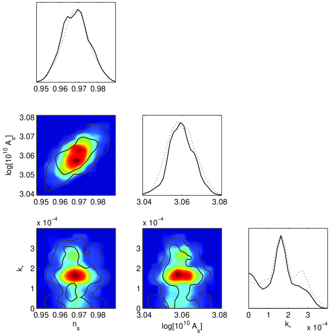
As it can be seen from Fig. 6, the parameters $A_{\text{s}}$ are $n_{\text{s}}$ are constrained from the both sides. Based on the fit to the WMAP data we find

$$n_{\text{s}} = 0.97\pm 0.07,$$

$$A_{\text{s}} = 2.1\cdot 10^{-9}\pm 0.1\cdot 10^{-9}.$$

These results are in agreement with (8) and (7). However it must be pointed out that they were computed at the different pivot scales.

The parameter $k_{*}$ has the upper constraint, however it is unbounded from below (large scales). It could be expected, since there is no observational data on the largest (greater than the Hubble radius) scales to get the upper constrain the parameter. Nevertheless some particular value of $k_{*}$ is privileged what leads to the peak in the probability distribution. Based on the fit to the WMAP data we have obtained following values of this parameter:

$$k_{*}=1.7\cdot 10^{-4}\pm 0.8\cdot 10^{-4}\ [\text{Mpc}^{-1}].$$

The length scale corresponding to $k_{*}$ is equal to

$$\lambda_{*}=\frac{2\pi}{k_{*}}\approx 4\cdot 10^{4}\ \text{Mpc}.$$ (34)

5 Big Bang vs. Big Bounce

In this section we compare the model with suppression with the standard inflationary model. The suppression appears generically within the Big Bounce cosmology. In turn, the slow-roll inflation in the standard Big Bang scenario does not lead to any suppression. While the suppression introduces a new length scale, the model with suppression has one more parameter in comparison with the standard case. The considered models are:

$H_{1}$ – The slow-roll inflation within the Big Bang cosmology (spectrum given by Eq. 1). This model has two parameters $A_{\text{s}}$ and $n_{\text{s}}$.

$H_{2}$ – The slow-roll inflation within the Big Bounce cosmology (spectrum given by Eq. 30). This model has three parameters $A_{\text{s}}$, $n_{\text{s}}$ and $k_{*}$.

In the Bayesian approach to model comparison the best model has the largest value of the so-called posterior probability in the light of data, which is defined in the following way [40]:

$$P(H_{i}|D)=\frac{P(D|H_{i})P(H_{i})}{P(D)}.$$ (35)

The $H_{i}$ stands for considered model and $D$ denotes data used in analysis. $P(H_{i})$ is the prior probability for the model under investigation, which should reflect all information which we have about it before the analysis with the data $D$, that comes from theoretical investigations, or from analysis with other data sets. In particular, if we have no foundation to favor of one model over another one, which is usually the case, we take equal values of $P(H_{i})$ for all considered models. $P(D|H_{i})$ is the marginalized likelihood function over the allowed parameters range, which we called evidence and is given by

$$E_{i}\equiv P(D|H_{i})=\int d\hat{\theta}L(\hat{\theta})P(\hat{\theta}|H_{i}).$$ (36)

The $\hat{\theta}$ denotes vector of model parameters, $L(\hat{\theta})$ is the likelihood function for considered model and $P(\hat{\theta}|H_{i})$ is the prior probability distribution function for model parameters.

It is convenient to consider the ratio of models probabilities, which is reduced to the evidence ratio (so called Bayes factor) when all considered models have equal prior probabilities:

$$B_{ij}=\frac{E_{i}}{E_{j}}.$$ (37)

Their values give us information about the strength of evidence in favor of better model [41]: if $0<\ln B<1$ we could not give conclusive answer, if $1<\ln B<2.5$ there is weak evidence, if $2.5<\ln B<5$ the evidence is moderate, and for $\ln B>5$ evidence is strong.

The values of evidence for two alternative models of primordial perturbation spectrum was calculated with the help of CosmoClust code, which was introduced by [39] as a part of CosmoMC code. We have based on anisotropy (TT) and polarization (TE, EE) data from the WMAP satellite. In computations, we have neglected the contribution from the tensor power spectrum (we set $\mathcal{P}_{\text{t}}(k)=0$).

We assume that models are equally probable ($P(H_{1})=P(H_{2})=1/2$). We consider flat prior probability distribution functions for unknown parameters in the following ranges: $A_{\text{s}}\in[1.5\cdot 10^{-9},5.5\cdot 10^{-9}]$, $n_{\text{s}}\in[0.5,1.5]$, $k_{*}\in[10^{-6},10^{-3}]$. The value of logarithm of the Bayes factor which was obtained in the analysis, i.e.

$$\ln(E_{1}/E_{2})=\ln B_{12}=0.2\pm 0.6,$$ (38)

does not give a conclusive answer. The data was not informative enough to distinguish these models. Therefore, in the light of the recent WMAP data the Big Bang and Big Bounce cosmologies are indistinguishable. The Big Bounce predictions are not in conflict with the observational data. Moreover, beside the fact that the Big Bounce model has one more parameter $k_{*}$, the obtained evidence is comparable with the Big Bang case.

The above result was obtained with use of the CosmoClust code which bases on the nested sampling method [42]. This method was applied also in the CosmoNest code [43]. The computations with use of CosmoNest gives $\ln B_{12}=1.1\pm 0.2$. Therefore a week evidence for Big Bang model is obtained. However, the CosmoNest was designed only for the case of the unimodal likelihood functions. In turn, the CosmoClust code extends to the case of the multi-modal likelihood functions. As it is clear from the bottom right panel in Fig. 6, the considered likelihood function (dotted line) is bimodal in the subspace $k_{*}$. The first peak is located at $k_{*}\sim 1.5\cdot 10^{-4}\text{Mpc}^{-1}$ while the second at $k_{*}\sim 2.5\cdot 10^{-4}\text{Mpc}^{-1}$. Therefore the results from CosmoClust are more relevant for our model. The CosmoNest samples only around the highest peak, neglecting the contribution from the smaller one. Because of this, the observed discrepancy between the CosmoClust and CosmoNest results appears. It is worth to note that, the similar model with suppression on the large scales was shown as an example of use of the CosmoClust code [39]. The bimodality of the likelihood functions was also observed and applicability of the CosmoClust code to that cases was emphasized.

The issue of constraining the bouncing cosmology with the observational data was raised before in literature. In particular, studies based on SNIa data, location of acoustic peaks in the CMB and constraints from primordial nucleosynthesis (BBN) were performed in Ref. [44, 45]. However, these cosmographic methods are inefficient in searching for the effects of the bounce. It is due to the fact that the factor $\frac{\rho}{\rho_{\text{c}}}$ is extremely low at the energy scales covered with this method. Even during the BBN, where $T_{\text{BBN}}\sim 1$ MeV, we have $\rho_{\text{BBN}}\approx 10^{-90}\rho_{\text{Pl}}$. Therefore, if $\rho_{\text{c}}\approx\rho_{\text{Pl}}$, we have $\frac{\rho}{\rho_{\text{c}}}\approx 10^{-90}$ and the holonomy corrections in the Friedmann equation (2) are vanishingly small . Based on the method developed in the present paper, we reach $\rho_{\text{obs}}=\frac{m^{2}\phi^{2}_{\text{obs}}}{2}\approx 10^{-11}\rho_{\text{Pl}}$, what gives $\frac{\rho}{\rho_{\text{c}}}\approx 10^{-11}$ for $\rho_{\text{c}}\approx\rho_{\text{Pl}}$. Therefore, sensitivity on the holonomy corrections was increased around $10^{80}$ times with respect to the BBN constraint.

Based the the results presented in this section one can conclude that the Big Bounce is consistent with the observations up to energy scales $\approx 10^{-11}\rho_{\text{Pl}}$. In this region the Big Bounce and Big Bang cosmologies are indistinguishable in the light of the available observational data. The advantage of the Big Bounce model is however that the initial singularity problem is resolved and the initial conditions for the phase of inflation are naturally generated.

6 Can we see the Big Bounce?

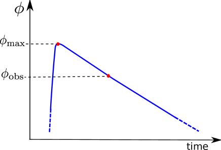
The present value of scale $\lambda_{*}$ is crucial from the point of possible observational investigations of the Big Bounce cosmology. As it was discussed before, this scale overlaps with the size of the Hubble radius at the beginning of inflation. Therefore, it corresponds to the point of maximal displacement of the inflaton field, namely $\phi_{\text{max}}$. In this section we investigate how the variation of $\phi_{\text{max}}$ influences on the present value of $\lambda_{*}$. Based on this, it will be possible to investigate the observational conditions on the bounce.

In Fig. 7, the schematic illustration of the scalar field evolution near the place of the maximal displacement was shown. In this figure we have marked the discussed $\phi_{\text{max}}$ value as well as the observed value $\phi_{\text{obs}}=2.9m_{\text{Pl}}$. While $\phi=\phi_{\text{obs}}$, the modes of the present size $\lambda_{0}=3.14$ Gpc (pivot scale) were formed. Based on this, we can determinate what is the present size of the mode, which was equal to the Hubble radius at $\phi=\phi_{\text{max}}$. The transition from $\phi=\phi_{\text{max}}$ to $\phi\approx 0$ corresponding to the total amount of $e$-foldings from inflation, which can be decomposed as follows $N_{\text{tot}}=\Delta N+N_{\text{obs}}$. Here $N_{\text{obs}}$ is the observed value which corresponds to the transition from $\phi=\phi_{\text{obs}}$ to $\phi\approx 0$. The number of $e$-foldings during the transition from $\phi_{\text{max}}$ to $\phi_{\text{obs}}$ can be expressed as follows

$$\Delta N=-\frac{4\pi}{m^{2}_{\text{Pl}}}\int_{\phi_{\text{max}}}^{\phi_{\text{obs}}}\frac{V}{V^{\prime}}d\phi=\frac{2\pi}{m^{2}_{\text{Pl}}}\left(\phi^{2}_{\text{max}}-\phi^{2}_{\text{obs}}\right).$$ (39)

Based on this expression as well as on the Friedmann equation, the present value of $\lambda_{*}$ can be expressed as follows

$$\lambda_{*}=\lambda_{0}\left(\frac{\phi_{\text{max}}}{m_{\text{Pl}}}\right)\left(\frac{m_{\text{Pl}}}{\phi_{\text{obs}}}\right)\exp\left\{2\pi\left(\frac{\phi_{\text{max}}}{m_{\text{Pl}}}\right)^{2}-2\pi\left(\frac{\phi_{\text{obs}}}{m_{\text{Pl}}}\right)^{2}\right\},$$ (40)

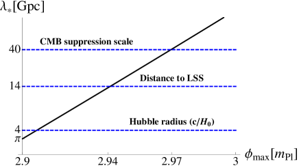
where $\lambda_{0}=3.14$ Gpc and $\phi_{\text{obs}}=2.9m_{\text{Pl}}$. In Fig. 8 we plot function $\lambda_{*}(\phi_{\text{max}})$ given by (40). For comparison, we also show some relevant length scales.

Figure 7: Schematic illustration of the scalar field evolution near the place of the maximal displacement. The $\phi_{\text{max}}$ is a maximal displacement of the field. The $\phi_{\text{obs}}$ is the value of the scalar field that corresponds to the powers spectrum measured at the pivot scale $\lambda_{0}=3.14$ Gpc.

The first one is the Hubble radius $H_{0}/c\approx 4$ Gpc. The second is the distance to last scattering shell (LSS), $D_{\text{LSS}}\approx 14$ Gpc. The last scale is the scale of suppression $\lambda_{*}\approx 40$ Gpc obtained in Sec. 5. If $\phi_{\text{max}}>2.94m_{\text{Pl}}$ then the scale $\lambda_{*}$ is placed behind the scale of LSS. In such a case there is no chance to see the effect of suppression directly. It is because, the scale of suppression is higher than the physical horizon of photons, released during the recombination. Therefore only if $\phi_{\text{max}}<2.94m_{\text{Pl}}$, there is a possibility to study the effects of suppression on the CMB. From the fit performed in Sec. 5 we got $\lambda_{*}\approx 40$ Gpc, what correspond to $\phi_{\text{max}}\approx 2.97m_{\text{Pl}}$. Based on this, the one particular evolutionary trajectory can be distinguished. However, one have to keep in mind that the probability distribution on the parameter $k_{*}$ was unbounded from below. Therefore the obtained value $\phi_{\text{max}}\approx 2.97m_{\text{Pl}}$ could be seen rather as a lower constraint on $\phi_{\text{max}}$. As mentioned, in order to make the direct observations of the suppression possible, the value of $\phi_{\text{max}}$ should be smaller than $2.94m_{\text{Pl}}$. The observations suggest that this value is higher, what unfortunately exclude this possibility. Based on this one can however exclude some models, where the predicted value of $\phi_{\text{max}}$ is not higher than $2.94m_{\text{Pl}}$. This is in fact a case for the symmetric inflation as studied in Ref. [8]. The issue of constraining this model was preliminary discussed in [9]. This is also still possible that the effect of oscillations can be observed. Perhaps it is even the reason why the particular value of $k_{*}$ was distinguished from the WMAP observations. Namely, it was possible because the structure of modulations at the low multipoles was reconstructed, not because the scale of suppression was detected.

Figure 8: The present value of the scale $\lambda_{*}$ as a function of $\phi_{\text{max}}$.

We finish this section with discussion of the observational constraint on the the parameter $\rho_{\text{c}}$. In loop quantum cosmology, total energy density is constrained by $\rho\leq\rho_{\text{c}}$. At the stage of inflation where the present pivot scale structure were initiated, the energy density is equal to

$$\rho_{\text{obs}}=\frac{m^{2}\phi^{2}_{\text{obs}}}{2}\approx 8\cdot 10^{-12}m^{4}_{\text{Pl}}.$$

Based on this, we infer that $\rho_{\text{c}}>\rho_{\text{obs}}$. Because $\rho_{\text{obs}}\ll\rho_{\text{Pl}}$, the observed constraint on the energy scale of the bounce is very weak. However, since $\rho_{\text{c}}\sim 1/\gamma^{3}$, the constraint on the parameter $\gamma$ can be much stronger. Indeed, based on (3) we find

$$\gamma<1100.$$ (41)

The value obtained from consideration of black hole entropy $\gamma=0.239$ places well within the observational bound. The constraint (41) is quite strong, however it must be kept in mind that it is based on relation (3), which can be invalid. As discussed in Ref. [13], the $\rho_{\text{c}}$ can be a free parameter, and then it would be impossible to put the constraint as (41). Therefore, more theoretical predictions regarding the phenomenological parameters as, $\rho_{\text{c}}$, are still awaiting.

To conclude, some models of the bouncing cosmology can be excluded based on the observations of CMB. It is based on the observational constraint on $\phi_{\text{max}}$. The direct observations of the bounce effects are however much harder to detect. As we have indicated, the effect of suppression cannot be used. It is because the scale of suppression was shown to be higher than the scale of horizon. The effect of oscillations gives a chance, however the effect is, in general, weaker and can be below the cosmic variance. It must be also pointed out that the discussed effects can be also predicted from the different models. Therefore the important task is to find the observable which enables to distinguish between the models.

7 Summary

In this paper we have examined observations of the cosmic microwave background radiation as the potential probe of physics in the Planck epoch. We have based our considerations on the predictions of loop quantum cosmology. Within this approach the initial singularity is replaced by a cosmic bounce. During the bounce, the universe reaches the maximal energy density $\rho_{\text{c}}<\infty$. In our studies, we have concentrated on the model with a massive scalar field. The advantage of this choice is that the phase of the standard slow-roll inflation is realized during the evolution. During this phase, the primordial perturbations are formed. Their properties can be investigated by observations of the CMB. Based on the recent results from the seven years of observations made by the WMAP satellite, we have determined some parameters of the model. In particular, we have found that inflaton mass $m=(1.4\pm 0.5)\cdot 10^{-6}m_{\text{Pl}}=(2.6\pm 0.6)\cdot 10^{13}$ GeV.

Subsequently, we have investigated the modifications of the primordial power spectrum due to presence of the bounce. The two main effects that were discussed are: suppression and oscillations of the inflationary spectrum. The suppression can very strongly modify the spectrum. However, the present scale of suppression was shown to be behind the Hubble radius. Therefore, the effect of suppression is not directly observationally available. Despite this, the present scale of suppression $\lambda_{*}=\frac{2\pi}{k_{*}}\approx 40\ \text{Gpc}$ was distinguished by the observations. This is because of the oscillations in the primordial power spectrum. The effect of oscillations is in general, more subtle and dominated by the cosmic variance. However, the present work indicates that the oscillations in the power spectrum can in fact explain the strong additional modulations in the spectrum of CMB on the low multipoles. In order to verify it, we have compared the Big Bounce model with the standard Big Bang scenario and showed that the present observational data is not informative enough to distinguish these models. In other words, the Big Bounce predictions were shown not to be in conflict with the observational data. Moreover, despite the Big Bounce model has one more parameter $k_{*}$, the evidence obtained in this case is comparable with the Big Bang case.

We have shown that $\phi_{\text{max}}$ is not lower than $2.97m_{\text{Pl}}$. Based on this, some models of the bounce, as the mentioned symmetric model, can be significantly constrained or even excluded. Assuming validity of (3) we gave an observational constraint on the Barbero-Immirzi parameter. We found that $\gamma<1100$. The corresponding constraint on $\rho_{\text{c}}$ was shown to be much weaker.