GRB spectral parameters within the fireball model

Abstract

Fireball model of the GRBs predicts generation of numerous internal shocks, which then efficiently accelerate charged particles and generate magnetic and electric fields. These fields are produced in the form of relatively small-scale stochastic ensembles of waves, thus, the accelerated particles diffuse in space due to interaction with the random waves and so emit so called Diffusive Synchrotron Radiation (DSR) in contrast to standard synchrotron radiation they would produce in a large-scale regular magnetic fields. In this paper we present first results of comprehensive modeling of the GRB spectral parameters within the fireball/internal shock concept. We have found that the non-perturbative DSR emission mechanism in a strong random magnetic field is consistent with observed distributions of the Band parameters and also with cross-correlations between them; this analysis allowed to restrict GRB physical parameters from the requirement of consistency between the model and observed distributions.

1 Introduction

The fireball model is currently accepted as a standard model of the gamma-ray burst (GRB) prompt emission (e.g., Mészáros, 2006). It is supposed that a central engine produces a number of relativistic internal shocks, which then interact with each other. The phenomenon of the shock waves requires an efficient mechanism of energy dissipation. In a collisionless case, the most efficient ways of the energy dissipation are via generation of fluctuating electromagnetic fields and acceleration of charged particles up to high energies.

Microscopically, this field generation can be driven by two-stream instabilities associated with the shock propagation (Kazimura et al., 1998; Medvedev & Loeb, 1999; Frederiksen et al., 2004; Bret et al., 2004, 2005; Nishikawa et al., 2003; Jaroschek et al., 2004; Hededal, 2005; Hededal & Nishikawa, 2005; Bret & Dieckmann, 2008; Keshet et al., 2008; Dieckmann & Bret, 2010), while the acceleration of particles is provided by their interaction with the shock-generated random and regular electromagnetic fields (Mészáros, 2002; Nishikawa et al., 2005; Piran, 2005; Sari, 2006; Silva, 2006). It is well established by now that the magnetic and electric fields produced in the shock interactions have often a significant random component at various spatial scales.

The presence of the random component is critically important for generation of nonthermal emission from corresponding objects. Indeed, unlike regular gyration in the presence of a regular magnetic field, the shock-accelerated charged particles moving through a plasma with random electromagnetic fields experience random Lorenz forces and so follow random trajectories representing a kind of spatial diffusion. Accordingly, the particles produce a diffusive radiation whose spectra depend on the type of the field (magnetic or electric) and on spectral energy distribution of the field over the spatial scales (Toptygin & Fleishman, 1987; Hededal, 2005; Fleishman, 2006; Fleishman & Bietenholz, 2007; Fleishman & Toptygin, 2007a; Sironi & Spitkovsky, 2009). Below in this paper we rely on analytical DSR theory proposed by Toptygin & Fleishman (1987) and then further developed by Fleishman (2006); Fleishman & Bietenholz (2007). An alternative way of calculating radiation is the use of numerical PIC simulations (Hededal, 2005; Hededal & Nishikawa, 2005; Nishikawa et al., 2008; Sironi & Spitkovsky, 2009), which confirm the analytical results in the common parameter domain. However, the case of strong random field and strong angular scattering of the radiating electrons requiring a large dynamic range of the involved parameters is yet beyond available PIC capacities, which justifies the choice in favor of the well tested analytical theory.

Individual spectra of the prompt GRB emission are typically well fitted by a phenomenological Band function (Band et al., 1993), which consists of low-energy (spectral index $\alpha$) and high-energy (spectral index $\beta$) power-law regions smoothly linked at a break energy $E_{br}$. The diffusive synchrotron radiation (DSR) was shown (Fleishman, 2006) to produce spectra consistent with that observed typically from the GRBs (Band et al., 1993; Mazets et al., 2004; Ohno et al., 2008; Pal’shin et al., 2008; Granot et al., 2009). It is yet unclear, however, if the DSR spectra are naturally consistent with observed distribution of the GRB spectral parameters (Preece et al., 2000; Kaneko et al., 2006) and what ranges of physical GRB parameters are needed to reconcile the theoretical spectra with the observed ones. In this paper we present a model of GRB prompt emission generation by DSR in relativistically expanding GRB jets. The input parameters of the model are constrained by available observations and take into account dependences between involved parameters implied by physical laws. We vary a number of free parameters of the model to achieve the best agreement between the variety of the modeled and observed spectra. This analysis confirms that the DSR model, specifically—the non-perturbative strong-field regime, is intrinsically consistent with the observed distributions of the GRB spectral parameters.

2 Formulation of the Model

To be specific we adopt the fireball model in which the GRB prompt emission is generated in a collimated jet ejected with a relativistically high speed $v$ from a central engine. Adopting a general internal shocks/fireball concept we accept that a single binary collision of relativistic internal shocks results in a single episode of the GRB prompt emission. Microscopically, this shock-shock interaction first produces high levels of random magnetic and/or electric fields and accelerates the charged particles up to large ultrarelativistic energies; and then, these particles interact with the random fields to generate the gamma-rays. Although there are some common general properties of all cases of relativistic shock interactions, each shock-shock collision is, nevertheless, unique in terms of combination of the physical parameters involved. Accordingly, we are going to estimate and adopt a set of standard (”mean”) parameters appropriate to account for the most global GRB properties, and then consider if a reasonable scatter of those standard parameters is capable of reproducing more detailed properties of the considered class of events as a whole—the statistical distributions of the GRB spectral parameters and cross-correlations between them. To do so, we consider a number of different emission models including the standard synchrotron radiation and DSR regimes in case of either weak or strong random magnetic field. The spectral slopes and breaks depend on both the emission mechanism and combination of physical parameters affecting the radiation spectra within a given mechanism. Thus, the goal of the modeling is to establish if there exists a parametric space making one or another theoretical model compatible with the observational data on the GRB spectral properties.

2.1 Basic parameters of the GRB source

From analysis of so-called ’compactness problem’, it is established that the bulk Lorenz-factor of the expanding jet $\Gamma=1/\sqrt{1-v^{2}/c^{2}}$, where $c$ is the speed of light, must be much larger than unity, $\Gamma\gtrsim 100$ (Paczynski & Rhoads, 1993; Piran, 2005; Sari, 2006). A maximum $\Gamma$ value is not well constrained observationally; being conservative, we will not consider values above 1000. The total kinetic energy of the jet is roughly $E\sim 10^{51}$ erg (Mészáros, 2006), which, along with $\Gamma$ estimate and an assumption of particle composition, allows estimating of the total number of ejected particles. We adopt that bulk of the jet mass resides in the protons, thus, the total number of ejected protons is estimated as

$$N=E/(\Gamma m_{p}c^{2})\sim 10^{51},$$ (1)

where $m_{p}$ is the proton (rest) mass. If no $e^{+}e^{-}$ pairs are produced, then the number of electrons is equal to the evaluated number of protons.

The number density of the particles is

$$n=\frac{N}{V},$$ (2)

where $V$ is the jet volume. The full volume occupied by the jet material is a cone with the opening angle $\Omega_{ang}$ (for the modeling we adopted a constant value of $\Omega_{ang}=10^{-3}$ ster), so $V_{cone}=(4\pi/3)\Omega_{\rm ang}R^{3}$, while the volume of spherical layer with thickness $\Delta$ of this cone is $V=(4\pi/3)\Omega_{ang}(R^{3}-(R-\Delta)^{3})$. The volume is not well constrained by the observations, although it can be estimated using observed time scale $\delta t$ of the emission variability. Indeed, for a relativistically moving source (e.g., Piran, 2005) we have $\delta t\approx\Delta/(2c\Gamma^{2})$; accordingly, for the co-moving frame we can estimate:

$$V^{\prime}=\frac{4\pi}{3}\Omega_{ang}\Delta^{\prime 3}=\frac{4\pi}{3}\Omega_{ang}8c^{3}\Gamma^{3}\delta t^{3}.$$ (3)

Then, the number density in the co-moving frame is

$$n^{\prime}=\frac{N}{V^{\prime}}.$$ (4)

The radiation spectra for each set of the source parameters are calculated in the co-moving system and then the emission frequency is transformed to the observer’s frame taking into account the relativistic motion of the source and cosmological expansion of the Universe

$$\omega^{\prime}=\frac{\omega}{2\Gamma}(1+z).$$ (5)

Let us introduce the energy contents (e.g., Sari, 2006) of constituents needed to produce radiation—the magnetic field

$$\epsilon_{B}\equiv\frac{U_{B}}{w}=\frac{B^{2}}{8\pi w},$$ (6)

where $w=\Gamma nm_{p}c^{2}$ is the kinetic energy density of the expanding shell and $U_{B}=\frac{B^{2}}{8\pi}$ is the energy density of the magnetic field; and accelerated electrons

$$\epsilon_{e}\equiv\frac{U_{e}}{w}=\frac{\gamma\xi_{e}m_{e}}{\Gamma m_{p}},$$ (7)

where $U_{e}=n_{e}\gamma\xi_{e}m_{e}c^{2}$ is the energy density of accelerated electrons, $\xi_{e}$ is a fraction of electrons being accelerated ($\xi_{e}<1$ if only a fraction of all electrons are accelerated (Bykov & Meszaros, 1996), while others remain ”cold”, and $\xi_{e}>1$ if $e^{+}e^{-}$ pairs are produced at the emission source), $\gamma$ is a characteristic Lorenz-factor of the accelerated electrons, and $m_{e}$ is the mass of electron.

2.2 Standard synchrotron model

Although synchrotron models are generally consistent with overall GRB energetics and light curves, they are intrinsically incompatible with the distribution of low-energy spectral index $\alpha$ (e.g., Baring & Braby, 2004). To demonstrate this explicitly, we show the model distribution of the low-energy indices obtained within a synchrotron model in Figure 1.

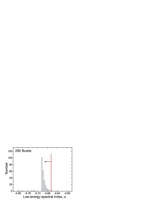
Figure 1: Model histogram of the spectral index distribution assuming slow cooling synchrotron regime. Note, that most of the indices are displaced by a small value compared with the asymptotic value, $-2/3$ (the ’line of death’). There are a number of outliers with a few of them apparently violating the ’line of death’. These outliers originate from the fit errors provided that the Band fitting function does not represent a perfect match to the theoretical synchrotron spectrum.

To be specific in generating this histogram we assumed the slow cooling regime and reasonable statistical distributions of the relevant parameters (see below for greater detail), such as bulk Lorentz factor of the relativistically expanding shell, energy content of the accelerated particles and produced magnetic field, number density of the particles, and their energy spectrum, as well as correlations between these parameters consistent with observations (Mészáros, 2006; Sari, 2006). The histogram in Fig. 1, representing an asymmetric narrow distribution peaking around $\alpha=-0.7$, is in evident contradiction with the observed one (Preece et al., 2000; Baring & Braby, 2004; Kaneko et al., 2006), which is a more or less symmetric broad distribution peaking at $\alpha\approx-1$. The fast cooling regime results in a histogram similar to that in Figure 1 with the only difference that it peaks around $\alpha\approx-1.5$. We conclude that a more sophisticated modeling is needed to achieve reasonable agreement between the observations and the theory of electromagnetic emission in the GRB sources. To address this problem, Medvedev (2000) proposed that emission of fast electrons moving in small-scale random magnetic field may possess the spectral properties consistent with those observed from GRBs; the corresponding DSR process in the GRB context has than been studied quantitatively by Fleishman (2006) within general concept of the stochastic theory of radiation proposed by Toptygin & Fleishman (1987).

2.3 Theory of DSR: main equations and parameters

For the purpose of this more detailed modeling we note that at the sites where the internal shocks interact in the GRB sources, charged particles are accelerated and two-stream instabilities produce high level of random magnetic and/or electric fields, so the diffusive synchrotron radiation (Fleishman, 2006) is expected to be produced there. Let us remind basic equations describing the DSR and main parameters determining its spectrum. We adopt that the energy of the random magnetic field is distributed over spatial scales according a power-law:

$$K_{\alpha\beta}(q_{0},\textbf{q})=\frac{1}{2}K(q_{0},\textbf{q})\left(\delta_{\alpha\beta}-\frac{k_{\alpha}k_{\beta}}{k^{2}}\right)=\frac{1}{2}K(\textbf{q})\delta(q_{0}-q_{0}(\textbf{q}))\left(\delta_{\alpha\beta}-\frac{k_{\alpha}k_{\beta}}{k^{2}}\right),$$ (8)

where

$$K(\textbf{q})=\frac{A_{\nu}}{q^{\nu+2}},\quad A_{\nu}=a_{\nu}q_{\min}^{\nu-1}\langle B_{\rm st}^{2}\rangle=\frac{(\nu-1)q_{\min}^{\nu-1}\langle B_{\rm st}^{2}\rangle}{4\pi},\quad q_{\min}<q<q_{\max},$$ (9)

$\nu$ is the spectral index of the random field distribution, the spectrum $K(\textbf{q})$ is normalized by $d^{3}q$ so that

$$\int_{q_{\min}}^{q_{\max}}K(\textbf{q})d^{3}q=\langle B_{\rm st}^{2}\rangle,\quad\quad q_{\min}\ll q_{\max},\nu>1,$$ (10)

$\langle B_{\rm st}^{2}\rangle$ is the mean square of the random magnetic field.

For the adopted spectrum of the random magnetic field, the perturbative DSR spectrum (Fleishman, 2006) can be obtained analytically:

$$I_{\omega}^{\bot}=\frac{8Q^{2}\gamma^{2}_{*}}{3\pi c}\cdot q(\omega),$$ (11)

where $\gamma_{*}^{-2}=\gamma^{-2}+\omega_{\rm pe}^{2}/\omega^{2}$,

$$q(\omega)=\left\{\begin{array}[]{ll}\frac{3\cdot 2^{\nu-1}\pi^{2}(\nu^{2}+3\nu+4)a_{\nu}}{\nu(\nu+2)^{2}(\nu+3)}\frac{\omega_{0}^{\nu-1}\omega_{\rm st}^{2}\gamma_{*}^{2\nu}}{\omega^{\nu}\gamma^{2}}\qquad\qquad\qquad\qquad\qquad\qquad\textrm{for }\omega<\frac{\omega_{\rm pe}^{2}}{2\omega_{0}}\ \textrm{or }\omega>2\gamma^{2}\omega_{0}\textrm{,}\\ \frac{\pi^{2}a_{\nu}\omega_{\rm st}^{2}}{2\nu\omega_{0}\gamma^{2}}\left[1+\frac{3\nu(\nu+1)\omega^{2}}{4(\nu+2)^{2}\gamma_{*}^{4}\omega_{0}^{2}}-\frac{\nu\omega^{3}}{2(\nu+3)\gamma_{*}^{6}\omega_{0}^{3}}+\frac{3\nu\omega^{2}}{4(\nu+2)\gamma_{*}^{4}\omega_{0}^{2}}\ln\left(\frac{\omega}{2\gamma_{*}^{2}k_{0}c}\right)\right]\ \textrm{for }\frac{\omega_{\rm pe}^{2}}{2\omega_{0}}\leq\omega\leq 2\gamma^{2}\omega_{0}\textrm{.}\end{array}\right.$$ (12)

These equations describe the DSR from particles moving along almost rectilinear trajectories and so valid only for relatively weak magnetic field. In the internal shock interactions, however, a strong random magnetic field can often be produced, which requires a more general, non-perturbative treatment (Fleishman, 2006; Fleishman & Bietenholz, 2007) in which the DSR spectrum has the form:

$$I_{\omega}=\frac{8Q^{2}q(\omega)}{3\pi c}\gamma^{2}\left(1+\frac{\omega_{\rm pe}^{2}\gamma^{2}}{\omega^{2}}\right)^{-1}\Phi(s),$$ (13)

where $\Phi(s)=24s^{2}\int_{0}^{\infty}dt\exp(-2st)\sin(2st)\left[\coth t-\frac{1}{t}\right]$ is the Migdal’s function, which depends on a single parameter $s=\frac{1}{8\gamma^{2}}\left(\frac{\omega}{q(\omega)}\right)^{1/2}\left(1+\frac{\omega_{\rm pe}^{2}\gamma^{2}}{\omega^{2}}\right)$; the scattering rate $q(\omega)$ has been defined by Eq. (12).

Therefore, the DSR intensity depends on the following (microscopic) parameters: the electron plasma frequency $\omega_{\rm pe}$, the (defined by the random field) gyrofrequency $\omega_{\rm st}$, the frequency $\omega_{0}=q_{\min}c$ specified by the main scale $L_{\max}=2\pi/q_{\min}$ of the random field spectrum, the spectral index $\nu$ of the random field, the Lorenz-factor $\gamma$ of the emitting relativistic electrons, and also on number (and spectral distribution) of the emitting electrons.

2.4 Links between microscopic and macroscopic parameters of GRBs

One of the difficulties in direct modeling of the GRB spectra is that they depend on microscopic parameters, which are basically unknown. However, we can link many of them with the macroscopic and phenomenological parameters of the GRB source introduced in § 2.1, (sf, e.g., Kumar & McMahon, 2008).

The electron plasma frequency is specified by the electron number density $n_{e}$

$$\omega_{\rm pe}=\sqrt{\frac{4\pi n_{e}e^{2}}{m_{e}}}.$$ (14)

Here we have to substitute the number density (4) found from the estimates of the total number of particles (1) and the source volume (3), then

$$\omega_{\rm pe}=\sqrt{\frac{4\pi Ne^{2}}{m_{e}V^{\prime}}}=\sqrt{\frac{4\pi e^{2}}{m_{e}V^{\prime}}\frac{E}{\Gamma m_{p}c^{2}}}=\sqrt{\frac{4\pi e^{2}}{m_{e}}\frac{3}{4\pi\Omega_{ang}R^{3}}\frac{E}{\Gamma m_{p}c^{2}}}=$$$$\sqrt{\frac{3e^{2}E}{m_{e}\Omega_{ang}(2c\delta t\Gamma)^{3}\Gamma m_{p}c^{2}}}=\sqrt{\frac{3e^{2}E}{8m_{e}\Omega_{ang}\delta t^{3}\Gamma^{4}m_{p}c^{5}}}$$ (15)

where $e$ and $m_{e}$ are the electron charge and mass, $m_{p}$ is the proton mass, $\delta t$ is the observed time of the emission variability, $\Omega_{ang}$ is the jet opening angle, and $E$ is the bulk kinetic energy of the shell. Therefore, the plasma frequency is expressed through a number of values, which can either be directly observed (like $\delta t$) or estimated from the observations (like $E$, $\Gamma$, and $\Omega_{ang}$).

Similarly, the stochastic gyrofrequency

$$\omega_{\rm st}^{2}=\frac{e^{2}\langle B_{\rm st}^{2}\rangle}{m_{e}^{2}c^{2}}$$ (16)

is defined by the random magnetic field value, and so can be expressed via the phenomenological parameter $\epsilon_{B}$ describing the energy content of the magnetic field:

$$\omega_{\rm st}=\sqrt{\frac{8\pi e^{2}\epsilon_{B}E}{m_{e}^{2}c^{2}V^{\prime}}}=\sqrt{\frac{8\pi e^{2}\epsilon_{B}E}{m_{e}^{2}c^{2}\frac{4\pi}{3}\Omega_{ang}(2c\delta t\Gamma)^{3}}}=\sqrt{\frac{3e^{2}\epsilon_{B}E}{4m_{e}^{2}c^{5}\Gamma^{3}\delta t^{3}}}.$$ (17)

The third parameter of the DSR spectrum having the dimension of frequency is $\omega_{0}=q_{\min}c=2\pi c/L_{\max}$, which is determined by the main scale of the random magnetic field distribution. To parameterize this unconstrained value we introduce a dimensionless model parameter $\Lambda=\omega_{0}/\omega_{\rm st}$ so that

$$\omega_{0}=\Lambda\cdot\omega_{\rm st}.$$ (18)

Then, $\Lambda\gg 1$ corresponds to a weak random field, while $\Lambda\ll 1$ to a strong random field.

Finally, the distribution of the magnetic energy over the spatial scales is determined by the spectral index $\nu$. We have no reliable constraint for this value from the GRB observation, however, using analogy with other astrophysical and laboratory cases, we adopt $1<\nu<2$.

Consider now parameters characterizing emitting relativistic electrons. The typical Lorenz-factor $\gamma$ of electrons can be expressed from Eq. (7) via parameters $\epsilon_{e}$, $\xi_{e}$, and $\Gamma$:

$$\gamma=\frac{\epsilon_{e}\Gamma m_{p}}{\xi_{e}m_{e}}.$$ (19)

Therefore, a single DSR spectrum is fully determined by specifying the following set of ten involved parameters: $E$, $\Gamma$, $\epsilon_{e}$, $\epsilon_{B}$, $\Lambda$, $\xi_{e}$, $\delta t$, $\Omega_{ang}$, $\nu$, and $z$. We turn now to specifying the corresponding parameter ranges.

2.5 Modeling strategy

For the sake of further modeling of the GRB spectra within the DSR emission model we note that the spectral parameters $\alpha$, $\beta$, and $E_{\rm break}$ of the Band fitting function display single-mode distributions. In terms of statistical properties of the GRB sources this implies that the GRB physical parameters are taken from the same parent distributions.

Therefore, we will perform a kind of ”global” statistical modeling of the GRB spectra. To do so we produce a large number ($\sim$5000) of individual DSR spectra, which differ from each other because different combination of input parameters is selected for each individual spectrum. Specifically, the ten independent parameters are randomly selected from the corresponding parent distributions, while the dependent (derived) parameters are then calculated as described in the previous section.

The independent parameters, where known, are taken based on observations available and the standard fireball model. For example, we adopt the total shell energy $E\sim 10^{51}$ erg, the jet opening angle $\Omega_{ang}\sim 10^{-3}$ ster, and $\Gamma\sim 300~{}(>100)$ to have normal distributions around the mean values, while the time variability scale $\delta t$ to have a log-normal distribution with the mean $\langle\delta t\rangle=10^{0}$ s and standard deviation $\sigma(\delta t)=10^{0.3}$ s as observed (Nakar & Piran, 2002). Parameters $\epsilon_{e}$ and $\epsilon_{B}$ are poorly constrained by observations; we kept them much less than unity in all cases, while consider a number of distributions for the spectral index $\nu$, which is also unknown parameter of the model. To reduce the number of free model parameters, we kept some parameters constant, which have only minor effect on the DSR spectrum shape; namely, we adopted $z=2$ and $\xi_{e}=1$.

Then, we made a simplifying assumption about the energy spectrum of the shock-accelerated electrons. Although this energy distribution is likely to be a broad one (for example, a power-law $n_{e}(E)\propto E^{-p}$), which can easily be taken into account, we adopt here a monoenergetic electron distribution. Indeed, adding the power-law energy distribution to the model would yield some spectrum regimes common for DSR and other competing emission processes including standard synchrotron radiation. We, however, want to evaluate the capability of the DSR mechanism itself to reproduce the Band function parameter distributions. If we succeed to do this with the monoenergetic distribution, then the power-law distribution will also be an acceptable one, since this will only increase (but not decrease) the variety of the produced radiation spectra; we return to this point later.

Finally, parameter $\Lambda$ is unknown. To evaluate the range of this parameter the most consistent with observed distributions of the GRB spectra, we vary it in a broad limits in our modeling from run to run, while keep a constant within each run.

3 Modeling results

3.1 Dependences of the DSR spectrum on the input parameters

Before turning to the statistical modeling described, it is worthwhile to consider how the DSR spectra depend on the independent input parameters. These dependences are not self-evident, because each input parameter (e.g., the bulk Lorenz-factor or bulk energy of the shell) affect a few microscopic parameters, which, in their turn, specify the DSR spectrum produced.

To do so, let us select the following set of ”standard” parameters $\Gamma=300$, $\epsilon_{e}=10^{-2}$, $\epsilon_{B}=10^{-4}$, $\Lambda=2$, $\xi_{e}=1$, $\delta t=1$ s, $\Omega_{ang}=10^{-3}$, $\nu=1.2$, and $z=2$ and then consider how the DSR spectrum changes as one of these parameters changes, while the others are kept the same.

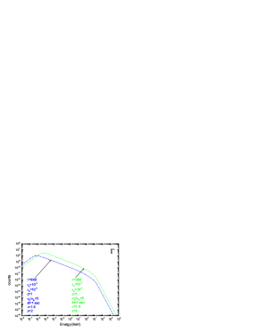
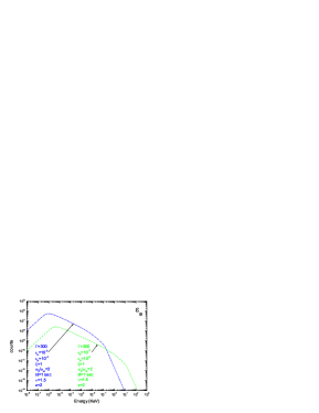
Figure 2: Change in the DSR spectrum due to bulk Lorenz-factor $\Gamma$ change.          

Figure 3: Change in the DSR spectrum due to $\epsilon_{e}$ change.

Figure 3 shows that the DSR level decreases and the spectrum moves towards lower energies as the bulk Lorenz-factor increases in contrast to simple expectation based on the bulk doppler shift only. The reason for such a behavior is that the bulk Lorenz-factor (for the same other input parameters) affects also other microscopic parameters, so the net effect of the $\Gamma$ change in the fireball model is different from purely kinematic Doppler effect. Increase of the relativistic electron energy content $\epsilon_{e}$ shifts the whole spectrum towards higher energies, Figure 3, since the main effect of $\epsilon_{e}$ increase is the corresponding increase of the typical Lorenz-factor $\gamma$ of the relativistic electrons.

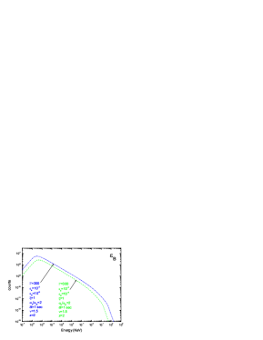
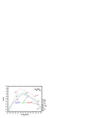
Figure 4: Change in the DSR spectrum due to $\epsilon_{B}$ change

Figure 5: Change in the DSR spectrum due to $\Lambda=\omega_{0}/\omega_{\rm st}$ change.

Figure 5 then displays that increase of the magnetic energy density, $\epsilon_{B}$, results basically in the upward shift of the whole spectrum and also to some shift of the high-frequency part of the spectrum towards higher energies. Parameter $\Lambda=\omega_{0}/\omega_{\rm st}$ has a major effect on the DSR spectrum Fig. 5 because it is the parameter that controls, which DSR regime, perturbative or non-perturbative, is in fact realized for a given parameter combination, i.e., weak or strong random magnetic field is present at the source. Accordingly, the DSR spectrum shape changes significantly as $\Lambda$ changes, new spectrum asymptotes arise as it decreases and non-perturbative DSR regime in a strong field develops.

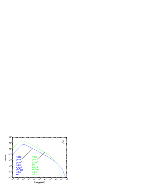
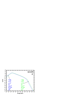
Figure 6: Change in the DSR spectrum due to $\xi_{e}$ change.

Figure 7: Change in the DSR spectrum due to $z$ change.

Decrease of the $\xi_{e}$ parameter results in a shift of the spectrum towards higher energies, Fig. 7. The reason for that is the same as at $\epsilon_{e}$ increase: according to Eq. (19) both of them lead to $\gamma$ increase and so to emission of correspondingly enhanced ($\propto\gamma^{2}$) energies. Increase of the cosmological red shift parameter shifts the whole spectrum towards lower energies, Fig. 7, as can be expected from the kinematics because no microscopic parameter depends on $z$ in this model.

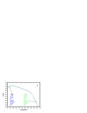
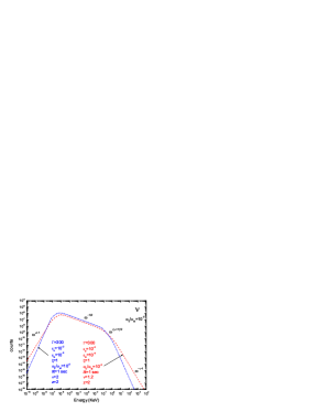
Figure 8: Change in the DSR spectrum due to $\nu$ change.

Finally, the spectral index $\nu$ of the random field affects the high-energy slope of the spectrum in the perturbative case, while affects other spectrum asymptotes as well in a more general, non-perturbative case, as can be seen from Figure 8. Now, when the important dependences of the DSR spectrum on the input parameters are established, we are in the position to perform the statistical modeling, and, to fine tune the parameter ranges towards model distributions matching the observed ones.

We start the modeling by adopting trial distributions for the parameters we are going to vary within a single run. Specifically, we initially adopt normal distributions for the involved parameters with the following means and standard deviations: $\langle\Gamma\rangle=300$, $\sigma_{\Gamma}=50$, $\langle\epsilon_{e}\rangle=10^{-2}$, $\sigma_{\epsilon_{e}}=10^{-4}$, $\langle\epsilon_{B}\rangle=10^{-4}$, $\sigma_{\epsilon_{B}}=10^{-6}$, $\langle\log_{10}\delta t\rangle=0$, $\sigma_{log_{10}\delta t}=3\cdot 10^{-1}$, $\langle\nu\rangle=1.2$, and $\sigma_{\nu}=5\cdot 10^{-2}$. Whenever possible, we will check if other than normal distribution offers a better fit to the observational data.

3.2 Case I: Week random magnetic field; perturbative treatment applies

We begin with the simplest case when the DSR spectrum can be described by a perturbative formulae derived in Fleishman (2006), which are widely used to evaluate the DSR in the perturbative (”jitter”) regime (see, e.g., Workman et al., 2008; Mao & Wang, 2007). The condition for random magnetic field to be weak is $\Lambda\equiv\omega_{0}/\omega_{\rm st}\gg 1$; then, applicability of the perturbative treatment requires additionally $\gamma<\omega_{\rm pe}\omega_{0}/\omega_{\rm st}^{2}$ (Fleishman, 2006). Adopting a constant value $\Lambda=10$ and taking randomly other involved parameters from the parent normal distributions described in the previous section, we generate around 5,000 individual DSR spectra, add noise to them at the level of 25$\%$, and fit each of them to the phenomenological Band function, see an example in Figure 9. This yields distributions of the spectral fitting parameters to be compared with the observed histograms of the Band parameters.

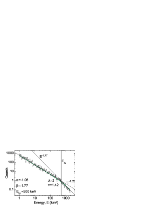
Figure 9: Example of the model noisy DSR spectrum (symbols, $\Lambda=2$, $\nu=1.42$) and fitting Band spectrum (solid thick green line). Thin solid lines display the low-energy and high-energy power-law asymptotes of the fitting Band function and position of the break energy; the Band parameters are shown in the left lower part of the figure. Note, that the adopted $\nu$ value would imply $\beta=-2.42$; however, relatively narrow region of the high-energy part of the spectrum and also added noise result in flatter asymptote with $\beta\approx-1.77$.

Figure 10 displays the model histograms. Remarkably, the model $E_{\rm break}$ histogram is very similar to the observed one, while the $\alpha$ and $\beta$ histograms display the peak values consistent with the observed ones ($-1$ and $-2.2$ respectively), although the widths of the model histograms are much smaller than of the observed ones. This inconsistency can be related to (i) use of the simplified perturbative treatment, (ii) non-optimal parameter range, or (iii) fundamental shortage of the adopted DSR model. We, thus, address these issues by applying full non-perturbative DSR treatment and exploring more complete range of the involved parameters. The remaining residuals between the model and observations will then be critically discussed within simplifications and limitations of the model used.

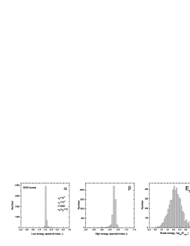
Figure 10: Histograms of the Band parameters $\alpha$, $\beta$, and $E_{\rm break}$ obtained within the perturbative (jitter) DSR model assuming the random magnetic field is weak.

3.3 Case II: Week random magnetic field; non-perturbative treatment

As is known (Toptygin & Fleishman, 1987; Fleishman, 2006) non-perturbative treatment may be required even for the case of relatively weak random field if the energy of radiating electron is large; it results in the $\propto\omega^{-1/2}$ asymptote, see, e.g., Figure 5. It is quite clear that an immediate outcome of this non-perturbative asymptote is appearance of $\alpha$ values around $-1/2$, so the range of $\alpha$ values between $-1$ and $-1/2$ will be filled. The distribution of individual $\alpha$ values in this range will change depending on the adopted $\Lambda=\omega_{0}/\omega_{\rm st}$ value.

Figure 11: Histograms of the Band parameters $\alpha$, $\beta$, and $E_{\rm break}$ obtained within the non-perturbative DSR model assuming the random magnetic field is weak, $\Lambda=1$.

Figure 11 displays an example of the Band parameter distributions obtained within the non-perturbative treatment for the case $\Lambda=1$, where the energy content of the magnetic field $\epsilon_{B}$ (and, accordingly, $\epsilon_{e}$, to keep $\epsilon_{e}=\sqrt{\epsilon_{B}}$, see, e.g., Sironi & Spitkovsky, 2009, and references therein) is increased to $\epsilon_{B}=10^{-3}$ to keep the break energy within the required window of observations. We see that the peak of the $\alpha$ histogram shifts to the value $\approx-0.6$, related to the $\propto\omega^{-1/2}$ asymptote. This histogram remains very narrow like in the perturbative case, and, furthermore, its peak value does not agree with the observed peak value any longer. Variation of parameter $\Lambda$ within the range corresponding to the weak field case, $\Lambda\geq 1$ does not improve the situation: the distribution remains narrow with the peak value between $-1$ and $-0.5$. We conclude that the DSR model with the weak random magnetic field, either perturbative or non-perturbative, cannot offer a consistent fit to the observed $\alpha$ histogram, while the model $E_{\rm break}$ histogram matches well the observed one. It is worthwhile to note here that a model with a weak random field was also criticized from another perspective (Kumar & McMahon, 2008) as it may imply an unrealistically high level of inverse Compton emission. In addition, Kirk & Reville (2010) argued that the weak-field case (needed to mediate the jitter-like regime of DSR) seems to be in contradiction with the required high efficiency of the particle acceleration at the shocks and strong magnetic fluctuations are needed to self-consistently accelerate electrons up to the gamma-ray producing energies. Thus, we turn now to the case of the strong random magnetic field.

3.4 Case III: Strong random magnetic field

Having the weak random field model (jitter regime) rejected, we turn now to analysis of the strong random field case, $\Lambda\leq 1$. As has been explained in § 3.1, new asymptotes, including $\propto\omega^{-(\nu+1)/2}$, arise in this case, which can yield broader $\alpha$ distribution if this new asymptote comes into play. Therefore, the model $\alpha$ distribution will depend on adopted $\nu$ distribution, which is in fact unconstrained by the observations. However, we can take advantage of the fact that in our model the $\beta$ distribution is straightforwardly determined by the $\nu$ distribution. Indeed, because $\beta=-\nu-1$, we can simply derive the required $\nu$ distribution from the observed $\beta$ distribution.

The observed $\beta$ histogram reaches the peak at around $-2.2$ and has asymmetric skew shape with a longer tail towards smaller values, which apparently cannot be described by a symmetric normal distribution adopted above. Thus, we have to adopt another reasonably simple distribution roughly matching the observed one. Specifically, we find that the Gamma distribution

$$F(\nu)=(\nu-\nu_{0})^{R-1}\cdot\frac{e^{-(\nu-\nu_{0})/b}}{b^{R}\Gamma(R)},$$ (20)

with $R=2$, where $\Gamma(R)$ is the Euler Gamma function, is well suited for our modeling. This distribution has a peak at $\nu=\nu_{0}+b$; we expect to obtain correct $\beta$ histogram for $\nu_{0}=0.9-1$ and $b=0.3-0.2$, see Figure 12.

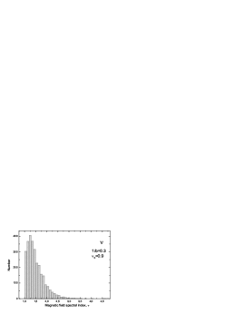
Figure 12: Example of Gamma distribution of the spectral index $\nu$ used in the modeling.

Other than the $\nu$ distribution adopted to obey Gamma distribution with the specified parameters, all other steps of the modeling are the same as before. We performed many runs changing the $\Lambda$ value and also varying other involved parameters within the adopted limits and found that typically the $\alpha$ distribution is much broader than in the case of the weak field considered in two previous sections in a general agreement with observations; the peak value of the $\alpha$ histogram varies between $-1.1$ and $-0.8$ when $\Lambda<1$. Figure 13 displays an example of the model Band spectral parameters obtained for the strong random field case.

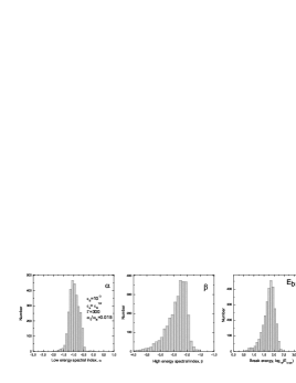
Figure 13: Example of the model Band parameter ($\alpha$, $\beta$, and $E_{\rm break}$) distributions obtained within the DSR model with strong random magnetic field.

The model results are in a remarkable agreement with the observations. Indeed, the $\alpha$ histogram is a symmetric one, it displays a peak at the right place, $\alpha=-1$, and its bandwidth is comparable to that of the observed histogram. The $\beta$ histogram almost repeats the observed one, displaying the correct asymmetric shape and the peak at the right place, $\beta=-2.2$. The $E_{\rm break}$ histogram agrees with the observed one rather well: it has correct shape and bandwidth, although the peak value is less than the observed value by the factor around 2. This discrepancy is, however, inessential: as we have seen in § 3.3, the position of the break energy can easily be adjusted by a small change of the magnetic energy content $\epsilon_{B}$ and corresponding change of $\epsilon_{e}$. Moreover, considering broader range of $\xi_{e}$ variation (recall, we adopted a constant value of $\xi_{e}=1$ in our modeling) can also easily change the characteristic break energy by a factor of 2 or more. Thus, we can conclude that the simplified DSR model adopted in this section is intrinsically capable of reproducing the Band parameter distributions compatible with the observed ones.

3.5 Cross-correlations between the model Band parameters

In addition to the Band parameter distributions themselves, it is worthwhile to address a question if our model reproduces the cross-correlations between the Band parameters correctly. This task can easily be solved using the variety of the model spectra produced in each model run.

Figure 14: Cross-correlation of the model Bend spectral parameters $\alpha$ and $\beta$.

Figure 15: Cross-correlation of the model Bend spectral index $\alpha$ and $E_{peak}=(\alpha+2)E_{0}$.

Figure 16: Cross-correlation of the model Bend spectral index $\beta$ and $E_{peak}=(\alpha+2)E_{0}$.

Figures 16–16 display these cross-correlations to be compared with Figure 31 from Kaneko et al. (2006). Like in the observation, the spectral indices $\alpha$ and $\beta$ are not highly correlated, although in the model plot the region of $-0.5<\alpha<0$ is underpopulated compared with the observed plot (Kaneko et al., 2006). Two other plots are in remarkable agreement with the observed cross-correlation plots, presented in Kaneko et al. (2006). We conclude that the developed model is naturally capable of reproducing the cross-correlation plots in addition to the histograms themselves, which is a remarkable success of the non-perturbative DSR model in the presence of strong random magnetic field.

4 Discussion

Our modeling shows that we can get an overall agreement between the model and observed histograms of the Band GRB spectral parameters within the non-perturbative DSR model with strong random magnetic field when $\Lambda\equiv\omega_{0}/\omega_{\rm st}\approx 0.015$. We note that in our model the $\Lambda$ parameter is not derived from a microscopic treatment of the shock interactions, rather it is a free model parameter adjusted for the model histogram to resemble the observed ones. Let us consider if the obtained $\Lambda$ value has any sense versus current models of magnetic field generation at the shock fronts. To do so we recall that $\omega_{0}$ is defined by the correlation length $L_{\max}$ of the random magnetic field, $\omega_{0}=2\pi c/L_{\max}$. If the magnetic field is produced by a two-stream (filamentation or Weibel) instability, the correlation length $L_{\max}$ is expected to be about ten plasma skin scales, $l_{sc}\sim 10c/\omega_{\rm pe}$ (e.g., Sironi & Spitkovsky, 2009). Since the frequencies $\omega_{\rm pe}$ and $\omega_{0}$ are independent input parameters in the modeling, we can check if the correlation length is indeed of the order of the skin scale, by inspecting the actual distribution of the $\omega_{0}/\omega_{\rm pe}$ ratio as it appears in the best-fit model case.

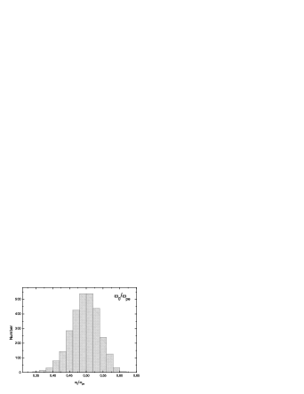
Figure 17: Histogram of the $\omega_{0}/\omega_{\rm pe}$ ratio derived from the DSR model with the strong random field with $\Lambda=0.015$.

Figure 17 displays a histogram of the $\omega_{0}/\omega_{\rm pe}$ ratio obtained for the model with $\Lambda=0.015$. The distribution has a symmetric bell shape with the peak about 0.5, thus, $L_{\max}\approx 4\pi l_{sc}$ and the required random field correlation length is indeed of the order of ten plasma skin scales, which agrees with the idea of the random field generation by a two-steam instability in the internal shock interactions.

We must note that although the model histograms and the cross-correlation plots look similar to the observed ones, there are some residuals between them. For example, the model $\alpha$ histogram is somewhat narrower than the observed one with a deficit of values $-2<\alpha<-1.5$ and $-0.5<\alpha<0$. The first interval can possibly be filled if one considers a nonuniformity of the emission source, which can naturally broaden the emission spectrum leading eventually to smaller $\alpha$ values. The second interval requires some additional physics, not included in our simplified modeling, to be taken into account, for example, random electric fields, turbulence anisotropy, or specific source geometry/viewing angle combination.

On the other hand, given the number of simplifying assumptions adopted for the modeling, we can conclude that the obtained agreement between the model and observations is remarkably good. Let us briefly remind and discuss those simplifications.

1. We considered random magnetic fields only. It is known, however, that diffusive radiation in electrostatic Langmuir waves results in a harder spectrum, e.g. $I_{\omega}\propto\omega^{1}$, (Fleishman & Toptygin, 2007a, b), thus, the presence of these Langmuir waves could compensate the deficit of the $-0.5<\alpha<0$ values.

2. A monoenergetic spectrum of accelerated electrons was adopted. Although typically the distribution of $\beta$ parameter is ascribed to a parent distribution of the spectral index $p$ of the electron distribution over energy, $N(E)\propto E^{p}$, our modeling shows that the right distribution of the $\beta$ index can easily be obtained even for a monoenergetic electron spectrum $N(E)\propto\delta(E-E_{*})$. In fact, for power-law energy distributions almost the same results hold for $p>2\nu+1$. However, if a power-law range with $p<2\nu+1$ is present in the electron energy spectrum, this is not in a contradiction with the model, although this does add more flexibility to formation of the $\beta$ distribution, which can further broaden it towards even better similarity to the observed histogram.

3. A number of the source parameters (e.g., $z$ and $\xi_{e}$) were adopted to be the same for all the sources; in fact, adopting more realistic distributions can broaden the obtained distributions of the Band spectral parameters and also affect the best-fit parameter space, so the accuracy of the obtained source parameters is at best to an order of magnitude.

4. Random magnetic fields accounted by the model were adopted to be statistically uniform and isotropic. Inclusion of the turbulence anisotropy can affect the radiation spectra and so modify the Band parameter distributions.

5. Having adopted both turbulence and electrons are isotropically distributed, we did not consider any source geometry/viewing angle effect. For the case of anisotropic distributions such effects can also come into play.

6. And finally, we did not explicitly consider the source evolution, although both particle distribution and magnetic field can evolve in time resulting in a GRB spectral evolution.

The latter three simplifications have in fact been addressed (e.g., Workman et al., 2008, and references therin) in a number of studies, however, a purely perturbative (jitter) weak-field regime of the DSR was adopted to calculate the radiation spectra. This weak-field regime was shown to rise severe problems in application to the GRB prompt emission (Kumar & McMahon, 2008; Kirk & Reville, 2010). In addition, as has been demonstrated above in this paper, this jitter regime of the DSR is inconsistent with the observed Band parameter distributions, while the strong-field regime is in fact needed. Since the strong-field regime requires a much more sophisticated fully non-perurbative treatment, those previous studies cannot be straightforwardly applied to this case, and so the required generalization must be specifically performed from scratch within the non-perturbative treatment (Toptygin & Fleishman, 1987; Fleishman, 2006; Fleishman & Bietenholz, 2007).

Although all these effects are potentially important and must eventually be taken into account in building a more comprehensive model, we conclude that even the simplified DSR model considered here is naturally capable of reproducing main characteristic properties of the Band parameter distributions and cross-correlations between them. The ranges of the parameters needed for the model to most closely reproduce the observed histograms agree well with standard fireball model parameters.

References

- Band et al. (1993) Band D., Matteson J., Ford L., Schaefer B., Palmer D., Teegarden B., Cline T., Briggs M., Paciesas W., Pendleton G., Fishman G., Kouveliotou C., Meegan C., Wilson R., Lestrade P., 1993, ApJ, 413, 281
- Baring & Braby (2004) Baring M. G., Braby M. L., 2004, ApJ, 613, 460
- Bret & Dieckmann (2008) Bret A., Dieckmann M. E., 2008, Physics of Plasmas, 15, 062102
- Bret et al. (2004) Bret A., Firpo M., Deutsch C., 2004, Phys. Rev. E, 70, 046401
- Bret et al. (2005) Bret A., Firpo M., Deutsch C., 2005, Physical Review Letters, 94, 115002
- Bykov & Meszaros (1996) Bykov A. M., Meszaros P., 1996, ApJ, 461, L37+
- Dieckmann & Bret (2010) Dieckmann M. E., Bret A., 2010, Phys. Scripta, 81, 015502
- Fleishman (2006) Fleishman G. D., 2006, ApJ, 638, 348
- Fleishman & Bietenholz (2007) Fleishman G. D., Bietenholz M. F., 2007, MNRAS, 376, 625
- Fleishman & Toptygin (2007a) Fleishman G. D., Toptygin I. N., 2007a, MNRAS, 381, 1473
- Fleishman & Toptygin (2007b) Fleishman G. D., Toptygin I. N., 2007b, Phys. Rev. E, 76, 017401
- Frederiksen et al. (2004) Frederiksen J. T., Hededal C. B., Haugbølle T., Nordlund Å., 2004, ApJ, 608, L13
- Granot et al. (2009) Granot J., Fermi LAT f. t., GBM collaborations 2009, ArXiv e-prints
- Hededal (2005) Hededal C., 2005, PhD thesis, , Niels Bohr Institute
- Hededal & Nishikawa (2005) Hededal C. B., Nishikawa K.-I., 2005, ApJ, 623, L89
- Jaroschek et al. (2004) Jaroschek C. H., Lesch H., Treumann R. A., 2004, ApJ, 616, 1065
- Kaneko et al. (2006) Kaneko Y., Preece R. D., Briggs M. S., Paciesas W. S., Meegan C. A., Band D. L., 2006, ApJS, 166, 298
- Kazimura et al. (1998) Kazimura Y., Sakai J. I., Neubert T., Bulanov S. V., 1998, ApJ, 498, L183
- Keshet et al. (2008) Keshet U., Katz B., Spitkovsky A., Waxman E., 2008, in 37th COSPAR Scientific Assembly Vol. 37 of COSPAR, Plenary Meeting, Evolution of magnetization in relativistic collisionless shocks. pp 1499–+
- Kirk & Reville (2010) Kirk J. G., Reville B., 2010, ApJ, 710, L16
- Kumar & McMahon (2008) Kumar P., McMahon E., 2008, MNRAS, 384, 33
- Mao & Wang (2007) Mao J., Wang J., 2007, ApJ, 669, L13
- Mazets et al. (2004) Mazets E. P., Aptekar R. L., Frederiks D. D., Golenetskii S. V., Il’Inskii V. N., Palshin V. D., Cline T. L., Butterworth P. S., 2004, in M. Feroci, F. Frontera, N. Masetti, & L. Piro ed., Astronomical Society of the Pacific Conference Series Vol. 312 of Astronomical Society of the Pacific Conference Series, Konus catalog of short GRBs. pp 102–+
- Medvedev & Loeb (1999) Medvedev M. V., Loeb A., 1999, ApJ, 526, 697
- Mészáros (2002) Mészáros P., 2002, ARA&A, 40, 137
- Mészáros (2006) Mészáros P., 2006, Reports on Progress in Physics, 69, 2259
- Nakar & Piran (2002) Nakar E., Piran T., 2002, MNRAS, 331, 40
- Nishikawa et al. (2003) Nishikawa K., Hardee P., Richardson G., Preece R., Sol H., Fishman G. J., 2003, ApJ, 595, 555
- Nishikawa et al. (2005) Nishikawa K., Hardee P., Richardson G., Preece R., Sol H., Fishman G. J., 2005, ApJ, 622, 927
- Nishikawa et al. (2008) Nishikawa K., Niemiec J., Sol H., Medvedev M., Zhang B., Nordlund Å., Frederiksen J., Hardee P., Mizuno Y., Hartmann D. H., Fishman G. J., 2008, in F. A. Aharonian, W. Hofmann, & F. Rieger ed., American Institute of Physics Conference Series Vol. 1085 of American Institute of Physics Conference Series, New Relativistic Particle-In-Cell Simulation Studies of Prompt and Early Afterglows from GRBs. pp 589–593
- Ohno et al. (2008) Ohno M., Fukazawa Y., Takahashi T., Yamaoka K., Sugita S., Pal’Shin V. e. a., 2008, PASJ, 60, 361
- Paczynski & Rhoads (1993) Paczynski B., Rhoads J. E., 1993, ApJ, 418, L5+
- Pal’shin et al. (2008) Pal’shin V., Aptekar R., Frederiks D., Golenetskii S., Il’Inskii V., Mazets E. e. a., 2008, in M. Galassi, D. Palmer, & E. Fenimore ed., American Institute of Physics Conference Series Vol. 1000 of American Institute of Physics Conference Series, Extremely long hard bursts observed by Konus-Wind. pp 117–120
- Piran (2005) Piran T., 2005, in AIP Conf. Proc. 784: Magnetic Fields in the Universe: From Laboratory and Stars to Primordial Structures. Magnetic Fields in Gamma-Ray Bursts: A Short Overview. pp 164–174
- Preece et al. (2000) Preece R. D., Briggs M. S., Mallozzi R. S., Pendleton G. N., Paciesas W. S., Band D. L., 2000, ApJS, 126, 19
- Sari (2006) Sari R., 2006, in P. A. Hughes & J. N. Bregman ed., Relativistic Jets: The Common Physics of AGN, Microquasars, and Gamma-Ray Bursts Vol. 856 of American Institute of Physics Conference Series, Gamma Ray Bursts and Their Afterglows. pp 33–56
- Silva (2006) Silva L. O., 2006, in Hughes P. A., Bregman J. N., eds, AIP Conf. Proc. 856: Relativistic Jets: The Common Physics of AGN, Microquasars, and Gamma-Ray Bursts. Physical Problems (Microphysics) in Relativistic Plasma Flows. pp 109–128
- Sironi & Spitkovsky (2009) Sironi L., Spitkovsky A., 2009, ArXiv e-prints
- Toptygin & Fleishman (1987) Toptygin I. N., Fleishman G. D., 1987, Astrophys. Space. Sci., 132, 213
- Workman et al. (2008) Workman J. C., Morsony B. J., Lazzati D., Medvedev M. V., 2008, MNRAS, 386, 199