QUARK–DIQUARK SYSTEMATICS OF BARYONS:
SPECTRAL INTEGRAL EQUATIONS FOR SYSTEMS COMPOSED BY LIGHT QUARKS

Abstract

For baryons composed by the light quarks ($q=u,d$) we write spectral integral equation using the notion of two diquarks: (i) axial–vector state, $D^{1}_{1}$, with the spin $S_{D}=1$ and isospin $I_{D}=1$ and (ii) scalar one, $D^{0}_{0}$, with the spin $S_{D}=0$ and isospin $I_{D}=0$. We present spectral integral equations for the $qD^{0}_{0}$ and $qD^{1}_{1}$ states taking into account quark–diquark confinement interaction.

PACS numbers: 11.25.Hf, 123.1K

1 Introduction

In the present paper we continue to investigate baryons as quark–diquark systems, $qD^{0}_{0}$ and $qD^{1}_{1}$. Here we consider in detail the systematization which was suggested in [1, 2].

In [2], a realistic classification of baryons was supposed. The introduction of diquarks allowed us to get a considerable decrease of excited states as compared to the quark model results of [3, 4, 5], though exceeding experimental data [6]. An additional decrease of states may be due to the overlap of $I=1/2$ states with $S=1/2$.

The classification obtained in [2] results in the linearity of trajectories in the $(J,M^{2})$ and $(n,M^{2})$ planes; the trajectories are strictly ordered. A particular feature of the scheme is the prediction of the number of overlapping poles. The observation of two-pole and three-pole structures in the complex-$M$ planes of partial amplitudes is a primary task in the verification of the scheme, while the next task consists in a writing and solving the spectral integral equation for quark–diquark systems with the aim to reconstruct the interaction. Such an equation should be similar to that written and solved before for the $q\bar{q}$ system [7].

Addressing the quark-diquark scheme, we suppose that the excited baryons do not prefer to be three-body systems of spatially separated colored quarks. Instead, similarly to mesons, they are two-body systems of quark and diquark: $q_{\alpha}D^{\alpha}=q_{\alpha}[\varepsilon^{\alpha\beta\gamma}q_{\beta}q_{\gamma}]$, where $\varepsilon^{\alpha\beta\gamma}$ is three-dimensional totally antisymmetrical tensor which works in color space. Below, we omit color indices imposing the symmetry anzatz for the spin–flavor–coordinate variables of wave functions.

It is an old idea that a $qq$-system inside the baryon can be regarded as a specific object – diquark. Thus, interactions with a baryon can be considered as interactions with quark, $q$, and two-quark system, $qq$: such a hypothesis was used in [8] for the description of the high-energy hadron–hadron collisions. In [9, 10, 11], baryons were described as quark–diquark systems. In hard processes on nucleons (or nuclei), the coherent $qq$ state (composite diquark) can be responsible for interactions in the region of large Bjorken-$x$ values, at $x\sim 2/3$; deep inelastic scatterings were considered in the framework of such an approach in [12, 13, 14, 15, 16]. More detailed considerations of the diquarks and their applications to different processes may be found in [17, 18, 19].

Here we concentrate our efforts on writing equations for pure $qD^{0}_{0}$ and $qD^{1}_{1}$ systems; the contribution of three-quark states is neglected. Spectral integral equations for $qD^{0}_{0}$ and $qD^{1}_{1}$ systems are shown in Fig. 1: the double line means diquark ($qD^{0}_{0}$ or $qD^{1}_{1}$), the flavor-neutral singular interaction is denoted by helix-type line. The flavor-neutrality of the interaction results in the absence of mixing of $qD^{0}_{0}$ and $qD^{1}_{1}$ states.

The further presentation is organized as follows. In section 2, we give the elements of technique, which are needed for writing spectral integral equations for $qD^{0}_{0}$ or $qD^{1}_{1}$ systems. In section 3, we discuss confinement singularities while in sections 4 and 5 we present the spectral integral equations.

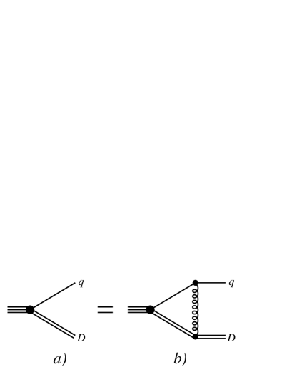
Figure 1: a,b) Equation for quark–diquark system (the flavor-neutral interaction denoted by helix-type line).

2 Technique for the description of fermions with large spin

Recall some necessary properties of angular momentum operators for two-particle systems and baryon projection operators. For more detail, see [20] and references therein.

2.1 Angular momentum operators for the two-particle systems

As in [20, 21], we use angular momentum operators $X^{(L)}_{\mu_{1}\ldots\mu_{L}}(k^{\perp})$, $Z^{\alpha}_{\mu_{1}\ldots\mu_{L}}(k^{\perp})$ and projection operator $O^{\mu_{1}\ldots\mu_{L}}_{\nu_{1}\ldots\nu_{L}}(\perp P)$. Let us recall their definition.

The operators are constructed from relative momenta $k^{\perp}_{\mu}$ and tensor $g^{\perp}_{\mu\nu}$. Both are orthogonal to the total momentum of the system:

$$k^{\perp}_{\mu}=\frac{1}{2}g^{\perp}_{\mu\nu}(k_{1}-k_{2})_{\nu}=k_{1\nu}g^{\perp P}_{\nu\mu}=-k_{2\nu}g^{\perp P}_{\nu\mu},\qquad g^{\perp}_{\mu\nu}\equiv g^{\perp P}_{\mu\nu}=g_{\mu\nu}-\frac{P_{\mu}P_{\nu}}{s}\;.$$ (1)

The operator for $L=0$ is a scalar (we write $X^{(0)}(k^{\perp})=1$) and the operator for $L=1$ is a vector, $X^{(1)}_{\mu}=k^{\perp}_{\mu}$. The operators $X^{(L)}_{\mu_{1}\ldots\mu_{L}}$ for $L\geq 1$ can be written in the form of a recurrence relation:

$$X^{(L)}_{\mu_{1}\ldots\mu_{L}}(k^{\perp}) = k^{\perp}_{\alpha}Z^{\alpha}_{\mu_{1}\ldots\mu_{L}}(k^{\perp}),$$

$$Z^{\alpha}_{\mu_{1}\ldots\mu_{L}}(k^{\perp}) = \frac{2L-1}{L^{2}}\Big{(}\sum^{L}_{i=1}X^{{(L-1)}}_{\mu_{1}\ldots\mu_{i-1}\mu_{i+1}\ldots\mu_{L}}(k^{\perp})g^{\perp}_{\mu_{i}\alpha}$$

$$-\frac{2}{2L-1}\sum^{L}_{i,\ell=1\atop i<\ell} g^{\perp}_{\mu_{i}\mu_{\ell}} X^{{(L-1)}}_{\mu_{1}\ldots\mu_{i-1}\mu_{i+1}\ldots\mu_{\ell-1}\mu_{\ell+1}\ldots\mu_{L}\alpha}(k^{\perp})\Big{)}.$$ (2)

We have the convolution equality $X^{(L)}_{\mu_{1}\ldots\mu_{L}}(k^{\perp})k^{\perp}_{\mu_{L}}=k^{2}_{\perp}X^{(L-1)}_{\mu_{1}\ldots\mu_{L-1}}(k^{\perp})$, with $k^{2}_{\perp}\equiv k^{\perp}_{\mu}k^{\perp}_{\mu}$, together with tracelessness property of $X^{(L)}_{\mu\mu\mu_{3}\ldots\mu_{L}}=0$. On this basis, one can write down the normalization condition for the angular momentum operators:

$$\int\frac{d\Omega}{4\pi}X^{(L)}_{\mu_{1}\ldots\mu_{L}}(k^{\perp})X^{(L^{\prime})}_{\mu_{1}\ldots\mu_{L}}(k^{\perp})=\alpha_{L}k^{2L}_{\perp}\;,\quad\alpha_{L}\ =\ \prod^{L}_{l=1}\frac{2l-1}{l},$$ (3)

where the integration is carried out over spherical variables: $\int d\Omega/(4\pi)=1$.

Iterating Eq. (2), one obtains the following expression for the operator $X^{(L)}_{\mu_{1}\ldots\mu_{L}}$ at $L\geq 1$:

$$X^{(L)}_{\mu_{1}\ldots\mu_{L}}(k^{\perp})=\alpha_{L}\Big{[}k^{\perp}_{\mu_{1}}k^{\perp}_{\mu_{2}}k^{\perp}_{\mu_{3}}k^{\perp}_{\mu_{4}}\ldots k^{\perp}_{\mu_{L}}-\frac{k^{2}_{\perp}}{2L-1}$$

$$\times\Big{(}g^{\perp}_{\mu_{1}\mu_{2}}k^{\perp}_{\mu_{3}}k^{\perp}_{\mu_{4}}\ldots k^{\perp}_{\mu_{L}}+g^{\perp}_{\mu_{1}\mu_{3}}k^{\perp}_{\mu_{2}}k^{\perp}_{\mu_{4}}\ldots k^{\perp}_{\mu_{L}}+\ldots\Big{)}+\frac{k^{4}_{\perp}}{(2L\!-\!1)(2L\!-\!3)}$$

$$\times\Big{(}g^{\perp}_{\mu_{1}\mu_{2}}g^{\perp}_{\mu_{3}\mu_{4}}k^{\perp}_{\mu_{5}}k^{\perp}_{\mu_{6}}\ldots k^{\perp}_{\mu_{L}}+g^{\perp}_{\mu_{1}\mu_{2}}g^{\perp}_{\mu_{3}\mu_{5}}k^{\perp}_{\mu_{4}}k^{\perp}_{\mu_{6}}\ldots k^{\perp}_{\mu_{L}}+\ldots\Big{)}+\ldots\Big{]}.$$ (4)

For the projection operators, one has:

$$O=1,\qquad O^{\mu}_{\nu}(\perp P)=g_{\mu\nu}^{\perp}\,,$$

$$O^{\mu_{1}\mu_{2}}_{\nu_{1}\nu_{2}}(\perp P)=\frac{1}{2}\left(g_{\mu_{1}\nu_{1}}^{\perp}g_{\mu_{2}\nu_{2}}^{\perp}\!+\!g_{\mu_{1}\nu_{2}}^{\perp}g_{\mu_{2}\nu_{1}}^{\perp}\!-\!\frac{2}{3}g_{\mu_{1}\mu_{2}}^{\perp}g_{\nu_{1}\nu_{2}}^{\perp}\right).$$ (5)

For higher states, the operator can be calculated, using the recurrent expression:

$$O^{\mu_{1}\ldots\mu_{L}}_{\nu_{1}\ldots\nu_{L}}(\perp P)=\frac{1}{L^{2}}\Big{(}\sum\limits_{i,\ell=1}^{L}g^{\perp}_{\mu_{i}\nu_{\ell}}O^{\mu_{1}\ldots\mu_{i-1}\mu_{i+1}\ldots\mu_{L}}_{\nu_{1}\ldots\nu_{\ell-1}\nu_{\ell+1}\ldots\nu_{L}}(\perp P)$$

$$-\frac{4}{(2L-1)(2L-3)}\times\sum\limits_{i<\ell\atop k<m}^{L}g^{\perp}_{\mu_{i}\mu_{\ell}}g^{\perp}_{\nu_{k}\nu_{m}}O^{\mu_{1}\ldots\mu_{i-1}\mu_{i+1}\ldots\mu_{\ell-1}\mu_{\ell+1}\ldots\mu_{L}}_{\nu_{1}\ldots\nu_{k-1}\nu_{k+1}\ldots\nu_{m-1}\nu_{m+1}\ldots\nu_{L}}(\perp P)\Big{)}.\qquad$$ (6)

The projection operators obey the relations:

$$O^{\mu_{1}\ldots\mu_{J}}_{\nu_{1}\ldots\nu_{L}}(\perp P)X^{(L)}_{\nu_{1}\ldots\nu_{L}}(k^{\perp}) = X^{(L)}_{\mu_{1}\ldots\mu_{L}}(k^{\perp})\,,$$

$$O^{\mu_{1}\ldots\mu_{L}}_{\nu_{1}\ldots\nu_{L}}(\perp P)k_{\nu_{1}}k_{\nu_{2}}\ldots k_{\nu_{L}} = \frac{1}{\alpha_{L}}X^{(L)}_{\mu_{1}\ldots\mu_{L}}(k^{\perp}).$$ (7)

Hence, the product of two $X^{L}(k_{\perp})$ operators results in the Legendre polynomials as follows:

$$X^{(L)(k_{\perp})}_{\mu_{1}\ldots\mu_{L}}(p^{\perp})(-1)^{J}O^{\mu_{1}\ldots\mu_{L}}_{\nu_{1}\ldots\nu_{L}}(\perp P)X^{(L)}_{\nu_{1}\ldots\nu_{L}}(k^{\perp})\!=\!\alpha_{L}(\sqrt{-p_{\perp}^{2}}\sqrt{-k_{\perp}^{2}})^{J}P_{L}(z),$$ (8)

where $z\equiv-(p^{\perp}k^{\perp})/(\sqrt{-p_{\perp}^{2}}\sqrt{-k_{\perp}^{2}})$.

2.2 Baryon projection operators

(i) Projection operators for particles with $J=1/2$.

It is convenient to use the baryon wave functions $u^{(a)}(p)$ and $\bar{u}^{(a)}(p)$, which are normalized as

$$\bar{u}^{(a)}(p)u^{(b)}(p)=\delta_{ab}$$ (9)

and obey the completeness condition

$$\sum_{a=1,2}u^{(a)}(p)\bar{u}^{(a)}(p)=\frac{m+\hat{p}}{2m}\,.$$ (10)

For a baryon with fixed polarization, one has to substitute:

$$\frac{m+\hat{p}}{2m}\to\frac{m+\hat{p}}{2m}\left(1+\gamma_{5}\hat{S}\right),$$ (11)

with the following normalization for the polarization vector $S^{2}=-1$ and the constraint $(pS)=0$.

(ii) Projection operators for particles with $J>1/2$.

The wave function of a particle with the momentum $p$, mass $m$ and spin $J=j+\frac{1}{2}$ is given by a four-spinor tensor $\Psi_{\mu_{1}\ldots\mu_{j}}$. It satisfies the constraints

$$(\hat{p}-M_{J^{P}})\Psi_{\mu_{1}\ldots\mu_{j}}=0,\quad p_{\mu_{i}}\Psi_{\mu_{1}\ldots\mu_{j}}=0,\quad\gamma_{\mu_{i}}\Psi_{\mu_{1}\ldots\mu_{j}}=0,$$ (12)

and the symmetry properties

$$\Psi_{\mu_{1}\ldots\mu_{i}\ldots\mu_{\ell}\ldots\mu_{j}} = \Psi_{\mu_{1}\ldots\mu_{\ell}\ldots\mu_{i}\ldots\mu_{j}}\;,$$

$$g_{\mu_{i}\mu_{\ell}}\Psi_{\mu_{1}\ldots\mu_{i}\ldots\mu_{\ell}\ldots\mu_{j}} = g^{\perp p}_{\mu_{i}\mu_{\ell}}\Psi_{\mu_{1}\ldots\mu_{i}\ldots\mu_{\ell}\ldots\mu_{j}}=0.$$ (13)

The equations (12), (2.2) define the structure of denominator of the fermion propagator (projection operator), which can be written in the following form:

$$\sum\limits_{a=1}^{2J+1}\Psi_{\mu_{1}\ldots\mu_{j}}^{(a)}\bar{\Psi}_{\mu_{1}\ldots\mu_{j}}^{(a)}\equiv F^{\mu_{1}\ldots\mu_{j}}_{\nu_{1}\ldots\nu_{j}}(p)=(-1)^{j}\frac{M_{J^{P}}+\hat{p}}{2M_{J^{P}}}R^{\mu_{1}\ldots\mu_{j}}_{\nu_{1}\ldots\nu_{j}}(\perp p)\ .$$ (14)

The operator $R^{\mu_{1}\ldots\mu_{j}}_{\nu_{1}\ldots\nu_{j}}(\perp p)$ describes tensor structure of the propagator. It is equal to 1 for the ($J=1/2$) particle and is proportional to $g^{\perp p}_{\mu\nu}-\gamma^{\perp}_{\mu}\gamma^{\perp}_{\nu}/3$ for the particle with spin $J=3/2$ (recall that $\gamma^{\perp}_{\mu}=g^{\perp p}_{\mu\nu}\gamma_{\nu}$).

The conditions (2.2) are the same for fermion and boson projection operators, therefore fermion projection operator can be written as follows:

$$R^{\mu_{1}\ldots\mu_{j}}_{\nu_{1}\ldots\nu_{j}}(\perp p)=O^{\mu_{1}\ldots\mu_{j}}_{\alpha_{1}\ldots\alpha_{j}}(\perp p)T^{\alpha_{1}\ldots\alpha_{j}}_{\beta_{1}\ldots\beta_{j}}(\perp p)O^{\beta_{1}\ldots\beta_{j}}_{\nu_{1}\ldots\nu_{j}}(\perp p)\ .$$ (15)

The operator $T^{\alpha_{1}\ldots\alpha_{j}}_{\beta_{1}\ldots\beta_{j}}(\perp p)$ can be expressed in a simple form, so all symmetry and orthogonality conditions are imposed by $O$-operators. First, the $T$-operator is constructed of metric tensors only, which act in the space of $\perp p$ and $\gamma^{\perp}$ matrices. Second, a construction like $\gamma^{\perp}_{\alpha_{i}}\gamma^{\perp}_{\alpha_{\ell}}=\frac{1}{2}g^{\perp}_{\alpha_{i}\alpha_{\ell}}+\sigma^{\perp}_{\alpha_{i}\alpha_{\ell}}$, with $\sigma^{\perp}_{\alpha_{i}\alpha_{\ell}}=\frac{1}{2}(\gamma^{\perp}_{\alpha_{i}}\gamma^{\perp}_{\alpha_{\ell}}-\gamma^{\perp}_{\alpha_{\ell}}\gamma^{\perp}_{\alpha_{i}}$), gives zero, when being multiplied by the $O^{\mu_{1}\ldots\mu_{j}}_{\alpha_{1}\ldots\alpha_{j}}$-operator: the first term is due to the tracelessness condition and the second one to symmetry properties. The only structures, which can be thus constructed, are $g^{\perp}_{\alpha_{i}\beta_{\ell}}$ and $\sigma^{\perp}_{\alpha_{i}\beta_{\ell}}$. Moreover, taking into account the symmetry properties of the $O$-operators, one can use any pair of indices from sets $\alpha_{1}\ldots\alpha_{j}$ and $\beta_{1}\ldots\beta_{j}$, for example, $\alpha_{i}\to\alpha_{1}$ and $\beta_{\ell}\to\beta_{1}$. Then,

$$T^{\alpha_{1}\ldots\alpha_{j}}_{\beta_{1}\ldots\beta_{j}}(\perp p)=\frac{j+1}{2j\!+\!1}\big{(}g^{\perp}_{\alpha_{1}\beta_{1}}-\frac{j}{j\!+\!1}\sigma^{\perp}_{\alpha_{1}\beta_{1}}\big{)}\prod\limits_{i=2}^{j}g^{\perp}_{\alpha_{i}\beta_{i}}.$$ (16)

Since $R^{\mu_{1}\ldots\mu_{n}}_{\nu_{1}\ldots\nu_{n}}(\perp p)$ is determined by convolutions of $O$-operators, see Eq. (15), we can replace in (16)

$$T^{\alpha_{1}\ldots\alpha_{j}}_{\beta_{1}\ldots\beta_{j}}(\perp p)\to T^{\alpha_{1}\ldots\alpha_{j}}_{\beta_{1}\ldots\beta_{j}}(p)=\frac{j+1}{2j\!+\!1}\big{(}g_{\alpha_{1}\beta_{1}}-\frac{j}{j\!+\!1}\sigma_{\alpha_{1}\beta_{1}}\big{)}\prod\limits_{i=2}^{j}g_{\alpha_{i}\beta_{i}}.$$ (17)

The coefficients in (17) are chosen to satisfy the constraints (12) and convolution condition:

$$F^{\mu_{1}\ldots\mu_{j}}_{\alpha_{1}\ldots\alpha_{j}}(p)F^{\alpha_{1}\ldots\alpha_{j}}_{\nu_{1}\ldots\nu_{j}}(p)=(-1)^{j}F^{\mu_{1}\ldots\mu_{j}}_{\nu_{1}\ldots\nu_{j}}(p)\;.$$ (18)

Spin projection operators are considered in a more detail in [20].

3 Confinement singularities

Confinement singularities were applied to the calculation of levels in meson sector, to $q\bar{q}$ systems [7] and heavy quark ones $Q\bar{Q}$ [22, 23]. Here we apply confinement singularities to the quark–diquark compound states.

(i) Meson sector

The linearity of the $q\bar{q}$-trajectories in the ($n,M^{2}$) planes in meson sector [24] (experimentally, up to large $n$ values, $n\leq 7$) provides us the $t$-channel singularity $V_{conf}\sim 1/q^{4}$ which creates the barrier $V_{conf}\sim r$ in the coordinate representation. The confinement interaction is two-component [7]:

$$V_{conf}=(I\otimes I)\,b_{S}\,r+(\gamma_{\mu}\otimes\gamma_{\mu})\,b_{V}\,r\ ,$$

$$b_{S}\simeq-b_{V}\simeq 0.15\,\,{\rm GeV}^{-2}\ .$$ (19)

The position of $q\bar{q}$ levels and data on radiative decays tell us that singular $t$-channel exchanges are necessary both in the scalar ($I\otimes I$) and vector ($\gamma_{\mu}\otimes\gamma_{\mu}$) channels. The $t$-channel exchange interactions (3) can take place both for white and color states, ${\bf c}={\bf 1}+{\bf 8}$, though, of course, the color-octet interaction plays a dominant role.

The spectral integral equation for the meson-$q\bar{q}$ vertex (or for $q\bar{q}$ wave function of the meson) was solved by introducing a cut-off into the interaction (3): $r\to re^{-\mu r}$. The cut-off parameter is small: $\mu\sim 1-10$ MeV; if $\mu$ is changing in this interval, the $q\bar{q}$-levels with $n\leq 7$ remain practically the same.

In [7, 22, 23], the spectral integral equations were solved in the momentum representation – this is natural, since we used dispersion integration technique (see discussion in [20]). In this representation, the interaction is re-written as follows:

$$re^{-\mu r}\to 8\pi\left(\frac{4\mu^{2}}{(\mu^{2}-q^{2}_{\perp})^{3}}-\frac{1}{(\mu^{2}-q^{2}_{\perp})^{2}}\right).$$ (20)

(ii) Quark–diquark sector

Bearing in mind that in the framework of spectral integration (as in dispersion technique) the total energy is not conserved, we have to write

$$q^{2}_{\perp}=(k^{\perp}_{1}-k^{{}^{\prime}\perp}_{1})_{\mu}(-k^{\perp}_{2}+k^{{}^{\prime}\perp}_{2})_{\mu}\$$ (21)

for the momentum transfer, where $k_{1}$ and $k_{2}$ are the momenta of the initial quark and diquark, while $k^{\prime}_{1}$ and $k^{\prime}_{2}$ are those after the interaction. The index $\perp$ means that we use components perpendicular to total momentum $p$ for the initial state and to $p^{\prime}$ for the final state:

$$k^{\perp}_{i\,\mu}=g^{\perp p}_{\mu\nu}k_{i\,\nu}\ ,\quad g^{\perp p}_{\mu\nu}=g_{\mu\nu}-\frac{p_{\mu}p_{\nu}}{p^{2}}\ ,\quad p=k_{1}+k_{2}\ ,\quad p^{2}=s\,,$$

$$k^{\prime\perp}_{i\,\mu}=g^{\perp p^{\prime}}_{\mu\nu}k^{\prime}_{i\,\nu}\ ,\quad g^{\perp p^{\prime}}_{\mu\nu}=g_{\mu\nu}-\frac{p^{\prime}_{\mu}p^{\prime}_{\nu}}{p^{{}^{\prime}2}}\ ,\quad p^{\prime}=k^{\prime}_{1}+k^{\prime}_{2}\,,\quad p^{\prime 2}=s^{\prime}.$$ (22)

Generally, we can write for the $t$-channel interaction block:

$$I_{N}(q^{2}_{\perp}) = \frac{4\pi(N+1)!}{(\mu^{2}-q^{2}_{\perp})^{N+2}}\sum^{N+1}_{n=0}\left(\mu+\sqrt{q^{2}_{\perp}}\right)^{N+1-n}\left(\mu-\sqrt{q^{2}_{\perp}}\right)^{n}$$ (23)

4 The $qD^{0}_{0}$ systems

First, let us present vertices for the transitions $N_{J^{P}}\to qD^{0}_{0}$ and the block of the confinement interaction (transition $qD^{0}_{0}\to qD^{0}_{0}$). Convoluting them, see Fig. 1, we obtain spectral integral equation for the $qD^{0}_{0}$ system. This equation is a modified Bethe–Salpeter equation [25] (see also [26, 27, 28]) re-written in terms of the dispersion integrals [29].

4.1 Vertices for the transition $N_{J^{P}}\to qD^{0}_{0}$

(i) The $N_{J^{+}}$ vertices with even $L$

The vertex for $J=L+1/2$ with even $L$ is equal to:

$$\Phi^{+}(k_{2})\bar{u}(k_{1})X^{(L)}_{\mu_{1}\ldots\mu_{L}}(k^{\perp})G^{(L,J^{+})}(k^{2}_{\perp})\psi_{(J^{+})\mu_{1}\ldots\mu_{j}}(p)$$

$$\equiv\Phi^{+}(k_{2})\bar{u}(k_{1})S_{\mu_{1}\ldots\mu_{j}}^{(L,J^{+})}(k_{1},k_{2})G^{(L,J^{+})}(k^{2}_{\perp})\psi_{(J^{+})\mu_{1}\ldots\mu_{j}}(p),\quad j=L,\quad$$ (24)

while for $J=L-1/2$ it is

$$\Phi^{+}(k_{2})\bar{u}(k_{1})i\gamma_{5}\gamma_{\nu}X^{(L)}_{\mu_{1}\ldots\mu_{L-1}\nu}(k^{\perp})G^{(J^{+})}(k^{2}_{\perp})\psi_{(J^{+})\mu_{1}\ldots\mu_{j}}(p)$$

$$\equiv\Phi^{+}(k_{2})\bar{u}(k_{1})S_{\mu_{1}\ldots\mu_{j}}^{(L,J^{+})}(k_{1},k_{2})G^{(L,J^{+})}(k^{2}_{\perp})\psi_{(J^{+})\mu_{1}\ldots\mu_{j}}(p),\quad j=L-1\,.\quad$$ (25)

(ii) The $N_{J^{-}}$ vertices with odd $L$

For odd $L$, the vertex for $J=L+1/2$ is equal to:

$$\Phi^{+}(k_{2})\bar{u}(k_{1})X^{(L)}_{\mu_{1}\ldots\mu_{L}}(k^{\perp})G^{(J^{-})}(k^{2}_{\perp})\psi_{(J^{-})\mu_{1}\ldots\mu_{j}}(p)$$

$$\equiv\Phi^{+}(k_{2})\bar{u}(k_{1})S_{\mu_{1}\ldots\mu_{j}}^{(L,J^{-})}(k_{1},k_{2})G^{(L,J^{-})}(k^{2}_{\perp})\psi_{(J^{+})\mu_{1}\ldots\mu_{j}}(p),\quad j=L,\quad$$ (26)

while for $J=L-1/2$:

$$\Phi^{+}(k_{2})\bar{u}(k_{1})i\gamma_{5}\gamma_{\nu}X^{(L)}_{\mu_{1}\ldots\mu_{L-1}\nu}(k^{\perp})G^{(J^{-})}(k^{2}_{\perp})\psi_{(J^{-})\mu_{1}\ldots\mu_{j}}(p)$$

$$\equiv\Phi^{+}(k_{2})\bar{u}(k_{1})S_{\mu_{1}\ldots\mu_{j}}^{(L,J^{-})}(k_{1},k_{2})G^{(L,J^{-})}(k^{2}_{\perp})\psi_{(J^{+})\mu_{1}\ldots\mu_{j}}(p),\quad j=L-1,\quad$$ (27)

We denote vertices (4.1)-(4.1) as follows:

$$G^{(L,J^{P})}_{qD^{0}_{0}}(k_{1},k_{2};p)=\Phi^{+}(k_{2})\bar{u}(k_{1})G^{(L,J^{P})}_{(qD^{0}_{0})\mu_{1}\ldots\mu_{j}}(k_{1},k_{2})\psi_{\mu_{1}\ldots\mu_{j}}^{(J^{P})}(p)$$

$$\equiv\Phi^{+}(k_{2})\bar{u}(k_{1})S^{(L,J^{P})}_{(qD^{0}_{0})\mu_{1}\ldots\mu_{j}}(k_{1},k_{2})G^{(L,J^{P})}_{qD^{0}_{0}}(k^{2}_{\perp})\psi_{\mu_{1}\ldots\mu_{j}}^{(J^{P})}(p),\quad j=J-\frac{1}{2}\,.\quad$$ (28)

The wave function of the $qD^{0}_{0}$ system reads:

$$\psi_{(qD^{0}_{0})\mu_{1}\ldots\mu_{j}}^{(L,J^{P})}(k_{1},k_{2})=S^{(L,J^{P})}_{(qD^{0}_{0})\mu_{1}\ldots\mu_{j}}(k_{1},k_{2})\frac{G^{(L,J^{P})}_{qD^{0}_{0}}(k^{2}_{\perp})}{s-M^{2}_{J^{P}}}$$

$$\equiv S^{(L,J^{P})}_{(qD^{0}_{0})\mu_{1}\ldots\mu_{j}}(k_{1},k_{2})\psi^{(L,J^{P})}_{qD^{0}_{0}}(s),$$ (29)

where $\psi^{(L,J^{P})}_{qD^{0}_{0}}(s)$ is its invariant part.

4.2 Confinement singularities in $qD^{0}_{0}$ interaction amplitude

Introducing the momenta of quarks and diquarks, we must remember that total energies are not conserved in the spectral integrals (like in dispersion relations). Hence, in general case $s\neq s^{\prime}$.

The interaction amplitude in the $qD^{0}_{0}$ system is written in the following form:

$${\rm S}:\quad\sum\limits_{N}\alpha^{(N)}_{S}(q^{2}_{\perp})\Big{(}\bar{u}(k_{1})\,I\,u(k^{\prime}_{1})\Big{)}\,I^{(\mu\to 0)}_{N}(q^{2}_{\perp})\Big{(}\Phi^{+}(k_{2})\Phi(k^{\prime}_{2})\Big{)},$$

$${\rm V}:\quad-\sum\limits_{N}\alpha^{(N)}_{V}(q^{2}_{\perp})\Big{(}\bar{u}(k_{1})\,\gamma_{\nu}\,u(k^{\prime}_{1})\Big{)}\,I^{(\mu\to 0)}_{N}(q^{2}_{\perp})\Big{(}\Phi^{+}(k_{2})\,(k_{2}+k^{\prime}_{2})_{\nu}\,\Phi(k^{\prime}_{2})\Big{)}.$$

Recall, the singular block, $I^{(\mu\to 0)}_{N}(q^{2}_{\perp})$, is given in (23), and the operator $\Phi(k_{2})$ refers to scalar diquarks.

Diquarks should be considered as composite particles, hence one can expect an appearance of form factors in the interaction block, correspondingly, $\alpha^{(N)}_{S}(q^{2}_{\perp})$ and $\alpha^{(N)}_{V}(q^{2}_{\perp})$.

The sum of interaction terms in (4.2) can be re-written in a compact form:

$$\Phi^{+}(k_{2})\bar{u}(k_{1})\,V_{D^{0}_{0}}^{q}(k_{1},k_{2};k^{\prime}_{1},k^{\prime}_{2})\,u(k^{\prime}_{1})\Phi(k^{\prime}_{2})$$ (31)

4.3 Spectral integral equation for $qD^{0}_{0}$ system

The spectral integral equation for $qD^{0}_{0}$ system reads (see Fig. 1):

$$\Phi^{+}(k_{2})\bar{u}(k_{1})G^{(L,J^{P})}_{(qD^{0}_{0})\mu_{1}\ldots\mu_{j}}(k_{1},k_{2})\psi_{\mu_{1}\ldots\mu_{j}}^{(J^{P})}(p)$$

$$= \Phi^{+}(k_{2})\bar{u}(k_{1})\int\limits^{\infty}_{(m+M_{D^{0}_{0}})^{2}}\frac{ds^{\prime}}{\pi}\frac{d\phi_{2}(P^{\prime};k^{\prime}_{1},k^{\prime}_{2})}{s^{\prime}-M^{2}_{L,J^{P}}}V_{D^{0}_{0}}^{q}(k_{1},k_{2};k^{\prime}_{1},k^{\prime}_{2})\frac{\hat{k}^{\prime}_{1}+m}{2m}$$ (32)

$$\qquad\qquad\qquad\qquad\qquad\qquad\times G^{(L,J^{P})}_{(qD^{0}_{0})\mu^{\prime}_{1}\ldots\mu^{\prime}_{j}}(k^{\prime}_{1},k^{\prime}_{2})\psi_{\mu^{\prime}_{1}\ldots\mu^{\prime}_{j}}^{(J^{P})}(p)\ .$$

Here, the interaction block (the right-hand side of (4.3)) is presented using the spectral (dispersion relation) integral over $ds^{\prime}$, and $d\phi_{2}(P^{\prime};k^{\prime}_{1},k^{\prime}_{2})$ is a standard phase-space integral for the $qD^{0}_{0}$ system in the intermediate state.

It is suitable to work with equation re-written in the following way:
(i) the left-hand and right-hand sides of Eq. (4.3) are convoluted with the spin operator of vertex (4.1),
(ii) the convoluted terms are integrated over final-state phase space of the $qD^{0}_{0}$ system:

$$d\phi_{2}(p;k_{1},k_{2})=\frac{1}{2}(2\pi)^{4}\delta^{(4)}(p-k_{1}-k_{2})\prod\limits_{a=1,2}\frac{d^{3}k_{a}}{(2\pi)^{3}2k_{a0}}\,.$$ (33)

We obtain:

$$\int d\phi_{2}(p;k_{1},k_{2})Sp\Big{[}S^{(L,J^{P})}_{(qD^{0}_{0})\nu_{1}\ldots\nu_{j}}(k_{1},k_{2})\frac{\hat{k}_{1}+m}{2m}G^{(L,J^{P})}_{(qD^{0}_{0})\mu_{1}\ldots\mu_{j}}(k_{1},k_{2})F_{\mu_{1}\ldots\mu_{j}}^{\nu_{1}\ldots\nu_{j}}(p)\Big{]}$$

$$=\int d\phi_{2}(p;k_{1},k_{2})Sp\Big{[}S^{(L,J^{P})}_{(qD^{0}_{0})\nu_{1}\ldots\nu_{j}}(k_{1},k_{2})\frac{\hat{k}_{1}+m}{2m}\int\limits^{\infty}_{(m+M_{D^{0}_{0}})^{2}}\frac{ds^{\prime}}{\pi}\frac{d\phi_{2}(P^{\prime};k^{\prime}_{1},k^{\prime}_{2})}{s^{\prime}-M^{2}_{L,J^{P}}}$$

$$\times V_{D^{0}_{0}}^{q}(k_{1},k_{2};k^{\prime}_{1},k^{\prime}_{2})\frac{\hat{k}^{\prime}_{1}+m}{2m}G^{(L,J^{P})}_{(qD^{0}_{0})\mu^{\prime}_{1}\ldots\mu^{\prime}_{j}}(k^{\prime}_{1},k^{\prime}_{2})F_{\mu^{\prime}_{1}\ldots\mu^{\prime}_{j}}^{\nu_{1}\ldots\nu_{j}}(p)\Big{]}.$$ (34)

The operators $F_{\mu_{1}\ldots\mu_{j}}^{\nu_{1}\ldots\nu_{j}}(p)$ and $S^{(L,J^{P})}_{(qD^{0}_{0})\mu_{1}\ldots\mu_{j}}(k_{1},k_{2})$ are given by Eqs. (14) and (4.1), correspondingly. We can re-write (4.3) incorporating the wave function $\psi^{(L,J^{P})}_{qD^{0}_{0}}(s)$, which is determined in Eq. (4.1):

$$\int d\phi_{2}(p;k_{1},k_{2})Sp\Big{[}S^{(L,J^{P})}_{(qD^{0}_{0})\nu_{1}\ldots\nu_{j}}(k_{1},k_{2})\frac{\hat{k}_{1}+m}{2m}S^{(L,J^{P})}_{(qD^{0}_{0})\mu_{1}\ldots\mu_{j}}(k_{1},k_{2})F_{\mu_{1}\ldots\mu_{j}}^{\nu_{1}\ldots\nu_{j}}(p)\Big{]}$$

$$\times(s-M^{2}_{J^{P}})\psi^{(L,J^{P})}_{(qD^{0}_{0})}(s)$$

$$= \int d\phi_{2}(p;k_{1},k_{2})Sp\Big{[}S^{(L,J^{P})}_{(qD^{0}_{0})\nu_{1}\ldots\nu_{j}}(k_{1},k_{2})\frac{\hat{k}_{1}+m}{2m}\int\limits^{\infty}_{(m+M_{D^{0}_{0}})^{2}}\frac{ds^{\prime}}{\pi}d\phi_{2}(P^{\prime};k^{\prime}_{1},k^{\prime}_{2})$$ (35)

$$\times V_{D^{0}_{0}}^{q}(k_{1},k_{2};k^{\prime}_{1},k^{\prime}_{2})\frac{\hat{k}^{\prime}_{1}+m}{2m}S^{(L,J^{P})}_{(qD^{0}_{0})\mu^{\prime}_{1}\ldots\mu^{\prime}_{j}}(k^{\prime}_{1},k^{\prime}_{2})\psi^{(L,J^{P})}_{(qD^{0}_{0})}(s^{\prime})F_{\mu^{\prime}_{1}\ldots\mu^{\prime}_{j}}^{\nu_{1}\ldots\nu_{j}}(p)\Big{]}.$$

5 Spectral integral equations for $qD^{1}_{1}$ systems with $I=3/2$

Here, we present equations for vertices, or wave functions, for the transitions $\Delta_{J^{P}}\to qD^{1}_{1}$ with $P=\pm$. Below, for the shake of simplicity, we consider $\Delta_{J^{P}}^{++}$ state: in this case it is necessary to take into account one quark–diquark channel only, namely, $uD^{1,I_{3}=3/2}_{1}$. We omit isotopic indices, denoting the quark–diquark state as $qD^{1}_{1}$.

5.1 Vertices for the transition $\Delta_{J^{P}}\to qD^{1}_{1}$

The $qD^{1}_{1}$ states are characterized by the total spin of the quark and diquark ($S=\frac{1}{2},\frac{3}{2}$), orbital momentum ($L$) and total angular momentum ($J$). The parity ($P$) is determined by $L$.

The systematization performed in [7] favors, in the first approximation, the consideration of quantum numbers $S$ and $L$ as good ones. Below, we follow this result.

Outgoing quark–diquark states with fixed $S$ read:

$$S=\frac{1}{2} : \quad\Phi_{\nu}^{+}(k_{2})\bar{u}(k_{1})i\gamma_{5}\gamma_{\nu}\frac{\hat{P}+\sqrt{s}}{\sqrt{s}}\equiv\Phi_{\nu}^{+}(k_{2})\bar{u}(k_{1})S^{1/2}_{\nu}(P)\ ,$$

$$S=\frac{3}{2} : \quad\Phi_{\nu}^{+}(k_{2})\bar{u}(k_{1})\big{(}-\frac{2}{3}g^{\perp P}_{\nu\mu}+\frac{1}{3}\sigma^{\perp P}_{\nu\mu}\big{)}\frac{\hat{P}+\sqrt{s}}{\sqrt{s}}\equiv\Phi_{\nu}^{+}(k_{2})\bar{u}(k_{1})S^{3/2}_{\nu\mu}(P)\ .\qquad$$ (36)

Here, we use the operator (4.2) for spins $1/2$ and $3/2$, substituting $M_{J^{P}}^{2}\to s$.

(i) The transition vertices $\Delta_{J^{\pm}}$ at $S=\frac{1}{2}$

The transition vertices for $J=L\pm 1/2$ read:

$$J=L+\frac{1}{2}\,:\quad\Phi^{+}_{\nu}(k_{2})\bar{u}(k_{1})S^{1/2}_{\nu}(P)X^{(L)}_{\mu_{1}\ldots\mu_{L}}(k^{\perp})G^{(S,L,J^{\pm})}(k^{2}_{\perp})\psi^{(J^{\pm})}_{\mu_{1}\ldots\mu_{j}}(p)$$

$$\equiv\Phi_{\nu}^{+}(k_{2})\bar{u}(k_{1})S_{\nu\mu_{1}\ldots\mu_{j}}^{(1/2,L,J^{\pm})}(k_{1},k_{2})G^{(S,L,J^{\pm})}(k^{2}_{\perp})\psi^{(J^{\pm})}_{\mu_{1}\ldots\mu_{j}}(p),\quad j=L\ ,$$

$$J=L-\frac{1}{2}\,:\quad\Phi_{\nu}^{+}(k_{2})\bar{u}(k_{1})S^{1/2}_{\nu}(P)\,i\gamma_{5}\gamma_{\nu^{\prime}}X^{(L)}_{\mu_{1}\ldots\mu_{L-1}\nu^{\prime}}(k^{\perp})G^{(S,L,J^{\pm})}(k^{2}_{\perp})\psi^{(J^{\pm})}_{\mu_{1}\ldots\mu_{j}}(p)$$

$$\equiv\Phi_{\nu}^{+}(k_{2})\bar{u}(k_{1})S_{\nu\mu_{1}\ldots\mu_{j}}^{(1/2,L,J^{\pm})}(k_{1},k_{2})G^{(S,L,J^{\pm})}(k^{2}_{\perp})\psi^{(J^{\pm})}_{\mu_{1}\ldots\mu_{j}}(p),\quad j=L-1\ .$$

Note that in (5.1), as in (4.1) and (4.1), we use the axial–vector operator $i\gamma_{5}\gamma_{\nu^{\prime}}$ for the decreasing rank of the vertex at fixed $L$; recall also that $P=+$ corresponds to even $L$ and $P=-$ to odd ones.

(ii) The transition vertices $\Delta_{J^{\pm}}$ at $S=\frac{3}{2}$

The transition vertices for $J=|{\bf L}+{\bf\frac{3}{2}}|$ and $P=(-1)^{L}$ are written as follows:

$$J=L+\frac{3}{2}:\quad\Phi_{\nu}^{+}(k_{2})\bar{u}(k_{1})S^{3/2}_{\nu\mu_{L+1}}(P)X^{(L)}_{\mu_{1}\ldots\mu_{L}}(k^{\perp})G^{(3/2,L,J^{\pm})}(k^{2}_{\perp})\psi^{(J^{\pm})}_{\mu_{1}\ldots\mu_{j}}(p)$$

$$\equiv\Phi_{\nu}^{+}(k_{2})\bar{u}(k_{1})S_{\nu\mu_{1}\ldots\mu_{j}}^{(3/2,L,J^{\pm})}(k_{1},k_{2})G^{(3/2,L,J^{\pm})}(k^{2}_{\perp})\psi^{(J^{\pm})}_{\mu_{1}\ldots\mu_{j}}(p),\quad j=L+1\ ,$$

$$J=L+\frac{1}{2}:\quad\Phi_{\nu}^{+}(k_{2})\bar{u}(k_{1})S^{3/2}_{\nu\mu_{L}}(P)i\gamma_{5}\gamma_{\nu_{1}}X^{(L)}_{\nu_{1}\mu_{1}\ldots\mu_{L-1}}(k^{\perp})G^{(3/2,L,J^{\pm})}(k^{2}_{\perp})\psi^{(J^{\pm})}_{\mu_{1}\ldots\mu_{j}}(p)$$

$$\equiv\Phi_{\nu}^{+}(k_{2})\bar{u}(k_{1})S_{\nu\mu_{1}\ldots\mu_{j}}^{(3/2,L,J^{\pm})}(k_{1},k_{2})G^{(3/2,L,J^{\pm})}(k^{2}_{\perp})\psi^{(J^{\pm})}_{\mu_{1}\ldots\mu_{j}}(p),\quad j=L\ ,$$

$$J=L-\frac{1}{2}:\quad\Phi_{\nu}^{+}(k_{2})\bar{u}(k_{1})S^{3/2}_{\nu\mu_{L-1}}(P)\prod\limits_{a=1}^{2}(i\gamma_{5}\gamma_{\nu_{a}})X^{(L)}_{\nu_{1}\nu_{2}\mu_{1}\ldots\mu_{L-2}}(k^{\perp})$$

$$\qquad\qquad\qquad\times G^{(3/2,L,J^{\pm})}(k^{2}_{\perp})\psi^{(J^{\pm})}_{\mu_{1}\ldots\mu_{j}}(p)$$

$$\equiv\Phi_{\nu}^{+}(k_{2})\bar{u}(k_{1})S_{\nu\mu_{1}\ldots\mu_{j}}^{(3/2,L,J^{\pm})}(k_{1},k_{2})G^{(3/2,L,J^{\pm})}(k^{2}_{\perp})\psi^{(J^{\pm})}_{\mu_{1}\ldots\mu_{j}}(p),\quad j=L-1\ ,$$

$$J=L-\frac{3}{2}:\quad\Phi_{\nu}^{+}(k_{2})\bar{u}(k_{1})S^{3/2}_{\nu\mu_{L-2}}(P)\prod\limits_{a=1}^{3}(i\gamma_{5}\gamma_{\nu_{a}})X^{(L)}_{\nu_{1}\nu_{2}\nu_{3}\mu_{1}\ldots\mu_{L-3}}(k^{\perp})$$ (38)

$$\qquad\qquad\qquad\times G^{(3/2,L,J^{\pm})}(k^{2}_{\perp})\psi^{(J^{\pm})}_{\mu_{1}\ldots\mu_{j}}(p)$$

$$\equiv\Phi_{\nu}^{+}(k_{2})\bar{u}(k_{1})S_{\nu\mu_{1}\ldots\mu_{j}}^{(3/2,L,J^{\pm})}(k_{1},k_{2})G^{(3/2,L,J^{\pm})}(k^{2}_{\perp})\psi^{(J^{\pm})}_{\mu_{1}\ldots\mu_{j}}(p),\quad j=L-2\ .\qquad$$

(iii) The invariant wave functions of the $qD^{1}_{1}$ systems

The invariant wave functions of the $qD^{1}_{1}$ systems are determined by vertices $G^{(S,L,J^{\pm})}(k^{2}_{\perp})$ as follows:

$$\frac{G^{(S,L,J^{\pm})}(k^{2}_{\perp})}{s-M^{2}_{S,L,J^{P}}}=\psi^{(S,L,J^{P})}_{qD^{1}_{1}}(s).$$ (39)

Recall that relative momentum squared $k^{2}_{\perp}$ depends on $s$ only.

5.2 Confinement singularities in $qD^{1}_{1}$ interaction block

Introducing the momenta of quarks and diquarks, we should remember that total energies are not conserved in the spectral integrals (just as in dispersion relations), so $s\neq s^{\prime}$.

The interaction amplitude for $qD^{1}_{1}$ system is written as follows.
S-exchange:

$$\Phi^{+}_{\nu}(k_{2})\bar{u}(k_{1})\,V_{qD^{1}_{1};\nu\nu^{\prime}}^{(S-ex)}(k_{1},k_{2};k^{\prime}_{1},k^{\prime}_{2})\,u(k^{\prime}_{1})\Phi_{\nu^{\prime}}(k^{\prime}_{2})$$ (40)

$$= \sum\limits_{N}\beta^{(N)}_{S}(q^{2}_{\perp})\Big{(}\bar{u}(k_{1})\,I\,u(k^{\prime}_{1})\Big{)}\,I^{(\mu\to 0)}_{N}(q^{2}_{\perp})\Big{(}\Phi_{\nu}^{+}(k_{2})g_{\nu\nu^{\prime}}\Phi_{\nu^{\prime}}(k^{\prime}_{2})\Big{)},$$

V-exchange:

$$\Phi^{+}_{\nu}(k_{2})\bar{u}(k_{1})\,V_{qD^{1}_{1};\nu\nu^{\prime}}^{(V-ex)}(k_{1},k_{2};k^{\prime}_{1},k^{\prime}_{2})\,u(k^{\prime}_{1})\Phi_{\nu^{\prime}}(k^{\prime}_{2})$$ (41)

$$= -\sum\limits_{N}\beta^{(1N)}_{V}(q^{2}_{\perp})\Big{(}\bar{u}(k_{1})\gamma_{\xi}u(k^{\prime}_{1})\Big{)}I^{(\mu\to 0)}_{N}(q^{2}_{\perp})\Big{(}\Phi_{\nu}^{+}(k_{2})g_{\nu\nu^{\prime}}\Phi_{\nu^{\prime}}(k^{\prime}_{2})\Big{)}(k_{2}+k^{\prime}_{2})_{\xi}$$

$$-\sum\limits_{N}\beta^{(2N)}_{V}(q^{2}_{\perp})\Big{(}\bar{u}(k_{1})\gamma_{\xi}u(k^{\prime}_{1})\Big{)}I^{(\mu\to 0)}_{N}(q^{2}_{\perp})\Big{[}\Phi_{\xi}^{+}(k_{2})\Big{(}k_{2\nu}g_{\nu\nu^{\prime}}\Phi_{\nu^{\prime}}(k^{\prime}_{2})\Big{)}$$

$$+\Big{(}\Phi_{\nu}^{+}(k_{2})g_{\nu\nu^{\prime}}k^{\prime}_{2\nu^{\prime}}\Big{)}\Phi_{\xi}(k^{\prime}_{2})\Big{]}.$$

We can re-write the sum of interaction terms in (40) in a compact form:

$$\Phi^{+}(k_{2})\bar{u}(k_{1})\,V_{qD^{1}_{1};\nu\nu^{\prime}}(k_{1},k_{2};k^{\prime}_{1},k^{\prime}_{2})\,u(k^{\prime}_{1})\Phi(k^{\prime}_{2}),$$ (42)

$$V_{qD^{1}_{1};\nu\nu^{\prime}}(k_{1},k_{2};k^{\prime}_{1},k^{\prime}_{2})=V_{qD^{1}_{1};\nu\nu^{\prime}}^{(S-ex)}(k_{1},k_{2};k^{\prime}_{1},k^{\prime}_{2})+V_{qD^{1}_{1};\nu\nu^{\prime}}^{(V-ex)}(k_{1},k_{2};k^{\prime}_{1},k^{\prime}_{2}).\qquad\qquad$$

5.2.1 Spectral integral equation for $qD^{1}_{1}$ system

The spectral integral equation for $qD^{1}_{1}$ system with fixed total spin $S=1/2,3/2$, orbital momentum $L$ and total angular momentum $J^{P}$ reads:

$$\Phi_{\nu}^{+}(k_{2})\bar{u}(k_{1})S_{\nu\mu_{1}\ldots\mu_{j}}^{(S,L,J^{P})}(k_{1},k_{2})G^{(S,L,J^{P})}(k^{2}_{\perp})\psi_{(J^{P})\mu_{1}\ldots\mu_{j}}(p)$$

$$=\Phi_{\nu}^{+}(k_{2})\bar{u}(k_{1})\int\limits^{\infty}_{(m+M_{D^{1}_{1}})^{2}}\frac{ds^{\prime}}{\pi}\frac{d\phi_{2}(P^{\prime};k^{\prime}_{1},k^{\prime}_{2})}{s^{\prime}-M^{2}_{S,L,J^{P}}}V_{qD^{1}_{1};\nu\nu^{\prime}}(k_{1},k_{2};k^{\prime}_{1},k^{\prime}_{2})\frac{\hat{k}^{\prime}_{1}+m}{2m}$$

$$\times S_{\nu^{\prime}\mu^{\prime}_{1}\ldots\mu^{\prime}_{j}}^{(S,L,J^{P})}(k^{\prime}_{1},k^{\prime}_{2})G^{(S,L,J^{P})}(k^{\prime 2}_{\perp})\psi_{\mu^{\prime}_{1}\ldots\mu^{\prime}_{j}}^{(J^{P})}(p).$$ (43)

Here, as in case of the $qD^{0}_{0}$ system, the interaction block (the right-hand side of (5.2.1)) is written with the use of spectral integral over $ds^{\prime}$, and $d\phi_{2}(P^{\prime};k^{\prime}_{1},k^{\prime}_{2})$ is the phase space, see Eq. (33), for the $qD^{1}_{1}$ system in the intermediate state.

As in Eq. (4.3), we can transform Eq. (5.2.1) convoluting the left-hand and right-hand sides with spin operator of vertices, see (5.1) and (5.1), and integrating the convoluted terms over final-state phase space of the $qD^{1}_{1}$ system, $d\phi_{2}(p;k_{1},k_{2})$. We obtain:

$$\int d\phi_{2}(p;k_{1},k_{2})Sp\Big{[}S^{(S,L,J^{P})}_{(qD^{1}_{1})\nu\nu_{1}\ldots\nu_{j}}(k_{1},k_{2})\frac{\hat{k}_{1}+m}{2m}S^{(S,L,J^{P})}_{(qD^{1}_{1})\nu\mu_{1}\ldots\mu_{j}}(k_{1},k_{2})F_{\mu_{1}\ldots\mu_{j}}^{\nu_{1}\ldots\nu_{j}}(p)\Big{]}$$

$$\times(s-M^{2}_{S,L,J^{P}})\psi^{(L,J^{P})}_{(qD^{1}_{1})}(s)$$

$$=\int d\phi_{2}(p;k_{1},k_{2})Sp\Big{[}S^{(S,L,J^{P})}_{(qD^{1}_{1})\nu\nu_{1}\ldots\nu_{j}}(k_{1},k_{2})\frac{\hat{k}_{1}+m}{2m}\int\limits^{\infty}_{(m+M_{D^{1}_{1}})^{2}}\frac{ds^{\prime}}{\pi}d\phi_{2}(P^{\prime};k^{\prime}_{1},k^{\prime}_{2})$$

$$\times V_{qD^{1}_{1};\nu\nu^{\prime}}(k_{1},k_{2};k^{\prime}_{1},k^{\prime}_{2})\frac{\hat{k}^{\prime}_{1}+m}{2m}S^{(S,L,J^{P})}_{(qD^{1}_{1})\nu^{\prime}\mu^{\prime}_{1}\ldots\mu^{\prime}_{j}}(k^{\prime}_{1},k^{\prime}_{2})\psi^{(L,J^{P})}_{(qD^{1}_{1})}(s^{\prime})F_{\mu^{\prime}_{1}\ldots\mu^{\prime}_{j}}^{\nu_{1}\ldots\nu_{j}}(p)\Big{]}.\quad\qquad$$ (44)

Figure 2: a) Confinement interaction taken into account in Eqs. (4.3) and (5.2.1); b,c) pion-exchange and quark-exchange interactions which are supposed to be small for highly excited $qD^{0}_{0}$ and $qD^{1}_{1}$ systems.

6 Conclusion

We have derived spectral integral equations for the simplest case, when quark–diquark system is a one-channel system: this is $qD^{0}_{0}$ for nucleon states and $qD^{1}_{1}$ for $\Delta_{J}$ states.

Considering quark–diquark states, we take into account the confinement interaction only (Fig. 2a) that is a rather rough approximation. Still, the above-performed classification of baryon states [1, 2] gives us a hint that such an approximation may work qualitatively. More precise results need including and investigating other interactions, for example, the pion and $u$-channel quark exchanges (Figs. 2b and 2c) as perturbative admixture – for more detail see discussion in [1].

References

- [1] A.V. Anisovich, V.V. Anisovich, M.A. Matveev, V.A. Nikonov, A.V. Sarantsev and T.O. Vulfs Searching for the quark-diquark systematics of baryons composed by the light quarks , arXiv: hep/ph-1001.1259.
- [2] A.V. Anisovich, V.V. Anisovich, M.A. Matveev, V.A. Nikonov, A.V. Sarantsev and T.O. Vulfs Quark-diquark systematics of baryons and the symmetry for the light states , arXiv: hep/ph-1002.1577.
-
[3]
N. Izgur and G. Karl, Phys. Rev. D18, 4187
(1978); D19, 2653 (1979);
S. Capstik, N. Izgur, Phys. Rev. D34, 2809 (1986). - [4] L.Y. Glozman et al., Phys. Rev. D58:094030 (1998).
- [5] U. Löring, B.C. Metsch, H.R. Petry, Eur.Phys. A10, 395 (2001); A10, 447 (2001).
- [6] C. Amsler et al. [Particle Data Group], Phys. Lett. B 667 (2008) 1.
- [7] V.V. Anisovich, L.G. Dakhno, M.A. Matveev, V.A. Nikonov, and A. V. Sarantsev, Yad. Fiz. 70, 480 (2007) [Phys. Atom. Nucl. 70, 450 (2007)].
- [8] V.V. Anisovich, Pis’ma ZhETF 2, 439 (1965) [JETP Lett. 2, 272 (1965)].
- [9] M. Ida and R. Kobayashi, Progr. Theor. Phys. 36, 846 (1966).
- [10] D.B Lichtenberg and L.J. Tassie, Phys. Rev. 155, 1601 (1967).
- [11] S. Ono, Progr. Theor. Phys. 48 964 (1972).
-
[12]
V.V. Anisovich, Pis’ma ZhETF 21 382 (1975) [JETP
Lett. 21, 174 (1975)];
V.V. Anisovich, P.E. Volkovitski, and V.I. Povzun, ZhETF 70, 1613 (1976) [Sov. Phys. JETP 43, 841 (1976)]. - [13] A. Schmidt and R. Blankenbeckler, Phys. Rev. D16, 1318 (1977).
- [14] F.E Close and R.G. Roberts, Z. Phys. C 8, 57 (1981).
- [15] T. Kawabe, Phys. Lett. B 114, 263 (1982).
- [16] S. Fredriksson, M. Jandel, and T. Larsen, Z. Phys. C 14, 35 (1982).
- [17] M. Anselmino and E. Predazzi, eds., Proceedings of the Workshop on Diquarks, World Scientific, Singapore (1989).
- [18] K. Goeke, P.Kroll, and H.R. Petry, eds., Proceedings of the Workshop on Quark Cluster Dynamics (1992).
- [19] M. Anselmino and E. Predazzi, eds., Proceedings of the Workshop on Diquarks II, World Scientific, Singapore (1992).
- [20] A.V. Anisovich, V.V. Anisovich, J. Nyiri, V.A. Nikonov, M.A. Matveev and A.V. Sarantsev, Mesons and Baryons. Systematization and Methods of Analysis, World Scientific, Singapore, 2008.
- [21] A.V. Anisovich, V.V. Anisovich, B.N. Markov, M.A. Matveev, and A. V. Sarantsev, J. Phys. G: Nucl. Part. Phys. 28, 15 (2002).
- [22] V.V. Anisovich, L.G. Dakhno, M.A. Matveev, V.A. Nikonov, and A. V. Sarantsev, Yad. Fiz. 70, 68 (2007) [Phys. Atom. Nucl. 70, 63 (2007)].
- [23] V.V. Anisovich, L.G. Dakhno, M.A. Matveev, V.A. Nikonov, and A.V. Sarantsev, Yad. Fiz. 70, 392 (2007) [Phys. Atom. Nucl. 70, 364 (2007)].
- [24] A.V. Anisovich, V.V. Anisovich, and A.V. Sarantsev, Phys. Rev. D 62:051502(R) (2000).
- [25] E. Salpeter and H.A. Bethe, Phys. Rev. 84, 1232 (1951).
- [26] H. Hersbach, Phys. Rev. C 50, 2562 (1994); Phys. Rev. A 46, 3657 (1992).
- [27] F. Gross and J. Milana, Phys. Rev. D 43, 2401 (1991).
- [28] K.M. Maung, D.E. Kahana, and J.W. Ng, Phys. Rev. A 46, 3657 (1992).
- [29] G.F. Chew and S. Mandestam, Phys. Rev. 119, 467 (1960).