An infinite-dimensional calculus for gauge theories

Abstract

A space for gauge theories is defined, using projective limits as subsets of Cartesian products of homomorphisms from a lattice on the structure group. In this space, non-interacting and interacting measures are defined as well as functions and operators. From projective limits of test functions and distributions on products of compact groups, a projective gauge triplet is obtained, which provides a framework for the infinite-dimensional calculus in gauge theories. The gauge measure behavior on nongeneric strata is also obtained.

1 Preliminaries

1.1 Gauge theory. Basic definitions

In its usual formulation a classical gauge theory consists of four basic objects:

(i) A principal fiber bundle $P\left(M,G\right)$ with structure group $G$ and projection $\pi:P\rightarrow M$, the base space $M$ being an oriented Riemannian manifold.

(ii) An affine space $\mathcal{C}$ of connections $\omega$ on $P$, modelled by a vector space $\mathcal{A}$ of 1-forms on $M$ with values on the Lie algebra $LG$ of $G$.

(iii) The space of differentiable sections of $P$, called the gauge group $\mathcal{G}$

(iv) A $\mathcal{G}-$invariant functional (the Lagrangian) $\mathcal{L}:\mathcal{A}\rightarrow\mathbb{R}$

The statement (iv) presumes the existence of a reference measure in the configuration space $\mathcal{A}/\mathcal{G}$, the exponential of the Lagrangian being a Radon-Nykodim derivative with respect to this reference measure. Because that might not always be possible to achieve, it is better to replace (iv) by:

(iv^′) A well defined measure in the configuration space $\mathcal{A}/\mathcal{G}$.

Choosing a reference connection, the affine space of connections on $P$ may be modelled by a vector space of $LG$-valued 1-forms ($C^{\infty}\left(\Lambda^{1}\otimes LG\right)$). Likewise the curvature $F$ is identified with an element of $C^{\infty}\left(\Lambda^{2}\otimes LG\right)$. In a coordinate system one writes

$$A=A_{\mu}^{a}dx^{\mu}t_{a}\qquad x\in M\qquad t_{a}\in LG$$

with the action of $\gamma=\{g\left(x\right)\}\in\mathcal{G}$ on $A\in\mathcal{A}$ given by

$$\gamma:A_{\mu}\left(x\right)\rightarrow\left(gA_{\mu}\right)\left(x\right)=g\left(x\right)A_{\mu}\left(x\right)g^{-1}\left(x\right)-\left(\partial g\right)\left(x\right)\cdot g^{-1}\left(x\right)$$ (1)

In this paper $G$ will always be considered to be a compact group.

The action of $\mathcal{G}$ on $\mathcal{A}$ leads to a stratification of $\mathcal{A}$ corresponding to the classes of equivalent orbits $\left\{gA;g\in\mathcal{G}\right\}$. Let $S_{A}$ denote the isotropy (or stabilizer) group of $A\in\mathcal{A}$

$$S_{A}=\left\{\gamma\in\mathcal{G}:\gamma A=A\right\}$$ (2)

The stratum $\Sigma\left(A\right)$ of $A$ is the set of connections having isotropy groups $\mathcal{G}-$conjugated to that of $A$

$$\Sigma\left(A\right)=\left\{B\in\mathcal{A}:\exists\gamma\in\mathcal{G}:S_{B}=\gamma S_{A}\gamma^{-1}\right\}$$ (3)

The configuration space of the gauge theory is the quotient space $\mathcal{A}/\mathcal{G}$ and therefore a stratum is the set of points in $\mathcal{A}/\mathcal{G}$ that correspond to orbits with conjugated isotropy groups.

1.2 Generalized connections and the Ashtekar-Lewandowski measure

Whenever a Lagrangian is defined the calculation of physical quantities in the path integral formulation

$$\left\langle\phi\right\rangle=\int_{\mathcal{A}/\mathcal{G}}\phi\left(\xi\right)e^{-\mathcal{L}\left(\xi\right)}d\mu\left(\xi\right)$$ (4)

requires a measure in $\mathcal{A}/\mathcal{G}$ and no such measure is found for Sobolev connections. Therefore it turned out to be more convenient to work in a space of generalized connections $\overline{\mathcal{A}}$, defining parallel transports on piecewise smooth paths as simple homomorphisms from the paths on $M$ to the group $G$, without a smoothness assumption[1]. The same applies to the generalized gauge group $\overline{\mathcal{G}}$. Then, there is in $\overline{\mathcal{A}}/\overline{\mathcal{G}}$ an induced Haar measure, the Ashtekar-Lewandowski (AL) measure[2] [3]. Sobolev connections are a dense zero measure subset of the generalized connections[4].

A generalized connection is simply a homomorphism from the groupoid of paths $\mathcal{P}$ to the structure group. Different choices for the groupoid of paths have been proposed. Piecewise analyticity was first proposed [5], later extended to the smooth category[6] and to a more general setting covering both cases [7] [8]. This led to the notions of graphs[2], webs and hyphs[9]. Here, being mostly concerned with the Yang-Mills theory (and not with gravity where diffeomorphism invariance is important), the piecewise analytic case will be considered.

The space of generalized connections is characterized by using the representation theory of $C^{\ast}$ algebras. The relevant algebra is the algebra $\mathcal{HA}$ of functions on $\mathcal{A}/\mathcal{G}$ obtained by taking finite linear combinations of finite products of traces of holonomies (Wilson loop functions $W_{\alpha}\left(A\right)$) around closed loops $\alpha$. The completion $\overline{\mathcal{HA}}$ of $\mathcal{HA}$ in the sup norm is a $C^{\ast}$ algebra. $\overline{\mathcal{HA}}$ is an abelian $C^{\ast}$ algebra and its Gel’fand spectrum is, by definition, the space of generalized connections $\overline{\mathcal{A}/\mathcal{G}}$ . An equivalence class of holonomically equivalent loops is called a hoop. By composition, hoops generate a hoop group $\mathcal{HG}$. Every point $\overline{A}\in\overline{\mathcal{A}/\mathcal{G}}$ gives rise to a homomorphism $\overset{\backsim}{H}$ from the hoop group $\mathcal{HG}$ to the structure group $G$ and every homorphism defines a point in $\overline{\mathcal{A}/\mathcal{G}}$ and, from $\overset{\backsim}{H}_{\overline{A}}\left(\beta\right)=TrH\left(\beta,\overline{A}\right)$, where $H\left(\beta,\overline{A}\right)$ denotes the holonomy, it follows that the correspondence has the trivial ambiguity that $\overset{\backsim}{H}$ and $g^{-1}\overset{\backsim}{H}g$ define the same point in $\overline{\mathcal{A}/\mathcal{G}}$ [5].

An important notion is the notion of independent hoops. Denote by $\overset{\backsim}{\alpha}$ the hoop for which $\alpha$ is a representative loop. In a set of independent hoops $\left\{\overset{\backsim}{\beta}_{1},\overset{\backsim}{\beta}_{2},\cdots,\overset{\backsim}{\beta}_{n}\right\}$ every representative loop $\beta_{i}$ must contain an open interval that is traversed exactly once and no finite segment of which is shared by any other loop in a different hoop. Furthermore given a set of hoops $\left\{\overset{\backsim}{\alpha}_{1},\overset{\backsim}{\alpha}_{2},\cdots,\overset{\backsim}{\alpha}_{k}\right\}$ it is always possible to find a set of independent hoops such that the hoop subgroup generated by the $\overset{\backsim}{\alpha}_{i}$’s is contained in the hoop subgroup generated by the $\overset{\backsim}{\beta}_{i}$’s and for every $\left(g_{1},g_{2},\cdots,g_{n}\right)\in G^{n}$ there is a connection $A\in\mathcal{A}$ such that $H\left(\beta_{i},A\right)=g_{i}$ , $i=1,\cdots,n$ [5]. $H\left(\beta_{i},A\right)$ denotes the holonomy $\left(W_{\beta}\left(A\right)=TrH\left(\beta_{i},A\right)\right)$.

The notion of independent hoops provides a simple definition of cylindrical functions. Given a set of independent loops $\beta_{1},\beta_{2},\cdots,\beta_{n}$, consider the hoop subgroup $S^{\ast}$ that they generate and define an equivalence relation in $\overline{\mathcal{A}/\mathcal{G}}$ by $\overline{A}_{1}\sim\overline{A}_{2}$ iff $\overset{\backsim}{H}_{\overline{A}_{1}}\left(\overset{\backsim}{\gamma}\right)=g^{-1}\overset{\backsim}{H}_{\overline{A}_{2}}\left(\overset{\backsim}{\gamma}\right)g$ for some $g\in G$ and all $\overset{\backsim}{\gamma}\in S^{\ast}$. Denoting by $\pi\left(S^{\ast}\right)$ the projection on the quotient space $\left(\overline{\mathcal{A}/\mathcal{G}}\right)/\backsim$, cylindrical functions are the pull-backs under $\pi\left(S^{\ast}\right)$ of the functions $f$ on $\left(\overline{\mathcal{A}/\mathcal{G}}\right)/\sim$. $\left(\overline{\mathcal{A}/\mathcal{G}}\right)/\sim$ is isomorphic to $G^{n}/Ad$ , the algebra of the cylindrical functions is a $C^{\ast}$ algebra and its completion in the sup norm is isomorphic to the algebra $\overline{\mathcal{HA}}$.

A natural integration measure for the cylindrical functions is the Haar measure on $G$, which being invariant under $G$, projects down naturally to $G^{n}/Ad$ . It satisfies the required compatibility condition in the sense that if $f$ is a cylindrical function on $\overline{\mathcal{A}/\mathcal{G}}$ with respect to two different finitely generated hoop subgroups $S_{i}^{\ast},i=1,2$, then

$$\int_{G^{n_{1}}/Ad}f_{1}d\mu_{1}=\int_{G^{n_{2}}/Ad}f_{2}d\mu_{2}$$

The measure on $\overline{\mathcal{A}/\mathcal{G}}$ whose restriction to cylindrical functions is the Haar measure on $G^{n}/Ad$ is the Ashtekar-Lewandowski measure.

1.3 Projective limits and physical interpretation

Let $\left\{I,\succ\right\}$ be a set endowed with an order relation $\succ$ and suppose that with each element $i\in I$ a set $X_{i}$ is associated and for each pair $\left(i,j\right)$, in which $j\succ i$, there is a mapping $\pi_{ij}:X_{j}\rightarrow X_{i}$ such that $\pi_{ii}$ is the identity and $\pi_{ki}\pi_{ij}=\pi_{kj}$. Then a set $X$ is called the projective limit$\mathcal{\ }X=\underset{\longleftarrow}{\lim}X_{i}$ of the family $\left\{X_{i}\right\}$ of sets if the following conditions are satisfied:

a) there is a family of mappings $\pi_{i}:X\rightarrow X_{i}$ such that for any pair $\left(i,j\right)$, in which $j\succ i$, $\pi_{ij}\pi_{j}=\pi_{i}$

b) for any family of mappings $\alpha_{i}:Y\rightarrow X_{i}$, from an arbitrary set $Y$, for which the equalities $\pi_{ij}\alpha_{j}=\alpha_{i}$ hold for $j\succ i$, there exists a unique mapping $\alpha:Y\rightarrow X$ such that $\alpha_{i}=\pi_{i}\alpha$ for every $i\in I$.

An explicit construction of the projective limit, which is particularly suited to the physical interpretation is the following: Consider the direct product $\underset{i\in I}{\prod}X_{i}$ and select in it the subset $X$ which satisfies the consistency condition $j\succ i\Longrightarrow\pi_{ij}\overset{\backsim}{X}_{j}=\overset{\backsim}{X}_{i}$ with $\overset{\backsim}{X}_{i}\subset X_{i}$ and $\overset{\backsim}{X}_{j}\subset X_{j}$. This subset is the projective limit of the family $\left\{X_{i}\right\}$ of sets.

Notice that this construction emphasizes the fact that the projective limit is not the limit of the sequence $X_{i}$. Instead it is a particular subset of the direct product. If, for example, the physical meaning of the index set $\left\{I,\succ\right\}$ is a refinement to successive smaller scales, the projective limit, once the consistency condition is fulfilled, contains a description of all the scales and not only the small scale limit.

2 The gauge projective space, kinematical measure, functions and operators

In the past, the Ashtekhar-Lewandowski measure has been constructed in very general settings, using projective limits of floating lattices and weak smoothness conditions. Here, staying closer to the usual physical setting of lattice gauge theory, one uses fixed square lattices with piecewise analytic parametrization.

Consider a sequence of square lattices in $\mathbb{R}^{4}$ of edge $\frac{a}{2^{k}}$ $k=0,1,2,\cdots$ constructed in such a way that the lattice of edge $\frac{a}{2^{k}}$ is a refinement of the $\frac{a}{2^{k-1}}$ lattice (all vertices of the $\frac{a}{2^{k-1}}$ lattice are also vertices in the $\frac{a}{2^{k}}$ lattice). Finite volume hypercubes $\Gamma$ in this lattice are a directed set $\left\{\Gamma,\succ\right\}$ under the inclusion relation $\succ$. $\Gamma\succ\Gamma^{\prime}$ meaning that all edges and vertices in $\Gamma^{\prime}$ are contained in $\Gamma$, the inclusion relation satisfies

$$\Gamma \succ \Gamma$$

$$\Gamma \succ \Gamma^{\prime}\text{ and }\Gamma^{\prime}\succ\Gamma\Longrightarrow\Gamma=\Gamma^{\prime}$$

$$\Gamma \succ \Gamma^{\prime}\text{ and }\Gamma^{\prime}\succ\Gamma^{\prime\prime}\Longrightarrow\Gamma\succ\Gamma^{\prime\prime}$$ (5)

For convenience one considers that the lattice refinement from size $\frac{a}{2^{k-1}}$ to $\frac{a}{2^{k}}$ is made one plaquette at a time so that all intermediate configurations are present in the directed set. This directed set will cover both successively higher volumes and finer and finer lattices. Let $p_{0}$ be a point that does not belong to any lattice of the directed family. One assumes an analytic parametrization of each edge, to each edge $l$ associates a $p_{0}$-based loop and for each generalized connection $A$ consider the holonomy $h_{l}\left(A\right)$.

For definiteness each edge is considered to be oriented along the coordinates positive direction and the set of edges of the lattice $\Gamma$ is denoted $E\left(\Gamma\right)$. The set $\mathcal{A}_{\Gamma}$ of generalized connections for the lattice hypercube $\Gamma$ is the set of homorphisms $\mathcal{A}_{\Gamma}=Hom\left(E\left(\Gamma\right),G\right)\sim G^{\#E\left(\Gamma\right)}$, obtained by associating to each edge the holonomy $h_{l}\left(\cdot\right)$ on the associated $p_{0}$-based loop. The set of gauge-independent generalized connections $\mathcal{A}_{\Gamma}/Ad$ is obtained factoring by the adjoint representation at $p_{0}$, $\mathcal{A}_{\Gamma}/Ad$ $\sim G^{\#E\left(\Gamma\right)}/Ad$. However because, for gauge independent functions, integration in $\mathcal{A}_{\Gamma}$ coincides with integration in $\mathcal{A}_{\Gamma}/Ad$ , for simplicity from now on one uses only $\mathcal{A}_{\Gamma}$. The space of generalized connections that one considers here is then the projective limit $\mathcal{A}=\underset{\longleftarrow}{\lim}\mathcal{A}_{\Gamma}$ of the family

$$\left\{\mathcal{A}_{\Gamma},\pi_{\Gamma\Gamma^{\prime}}:\Gamma^{\prime}\succ\Gamma\right\}$$ (6)

$\pi_{\Gamma\Gamma^{\prime}}$ and $\pi_{\Gamma}$ denote the surjective projections $\mathcal{A}_{\Gamma^{\prime}}\longrightarrow\mathcal{A}_{\Gamma}$ and $\mathcal{A}=\underset{\longleftarrow}{\lim}\mathcal{A}_{\Gamma}$.

Recall that the projective limit of the family $\left\{\mathcal{A}_{\Gamma},\pi_{\Gamma\Gamma^{\prime}}\right\}$ is the subset $\mathcal{A}$ of the Cartesian product $\underset{\Gamma}{\prod}\mathcal{A}_{\Gamma}$ that satisfies the consistent condition

$$\mathcal{A}=\left\{a\in\underset{\Gamma}{\prod}\mathcal{A}_{\Gamma}:\Gamma^{\prime}\succ\Gamma\Longrightarrow\pi_{\Gamma\Gamma^{\prime}}\mathcal{A}_{\Gamma^{{}^{\prime}}}=\mathcal{A}_{\Gamma}\right\}$$

The projective topology in $\mathcal{A}$ is the coarsest topology for which each $\pi_{\Gamma}$ mapping is continuous.

For a compact group $G$, each $\mathcal{A}_{\Gamma}$ is a compact Hausdorff space. Then $\mathcal{A}$ is also a compact Hausdorff space. In each $\mathcal{A}_{\Gamma}$ one has a natural (Haar) normalized product measure $\nu_{\Gamma}=\mu_{H}^{\#E\left(\Gamma\right)}$, $\mu_{H}$ being the normalized Haar measure in $G$. Then, according to a theorem of Prokhorov, as generalized by Kisynski[10] [11], if

$$\nu_{\Gamma^{\prime}}\left(\pi_{\Gamma\Gamma^{\prime}}^{-1}\left(B\right)\right)=\nu_{\Gamma}\left(B\right)$$ (7)

for every $\Gamma^{\prime}\succ\Gamma$ and every Borel set $B$ in $\mathcal{A}_{\Gamma}$, there is a unique measure $\nu$ in $\mathcal{A}$ such that $\nu\left(\pi_{\Gamma}^{-1}\left(B\right)\right)=\nu_{\Gamma}\left(B\right)$ for every $\Gamma$. Furthermore, this measure is tight, that is, for every $\varepsilon>0$ there is a compact subset $K$ of $\mathcal{A}$ such that $\nu_{\Gamma}\left(\mathcal{A}_{\Gamma}-\pi_{\Gamma}\left(K\right)\right)<\varepsilon$. The measure $\nu$, so constructed, is a version of the Ashtekar-Lewandowski measure.

The consistency condition (7) is easy to check in the present context. It suffices to consider $\Gamma^{\prime}=\Gamma_{k}$ as the refinement of $\Gamma=\Gamma_{k-1}$ when the edge size goes from $\frac{a}{2^{k-1}}$ to $\frac{a}{2^{k}}$. Then, if $g_{i}$ are group elements associated to the finer lattice (size $\frac{a}{2^{k}}$)

$$\nu_{k-1}\left(g_{1}\times g_{2}\times g_{3}\times g_{4}\in B\right) = \nu_{k-1}\left(g_{i}\times g_{j}\times g_{k}\times\left(g_{i}\times g_{j}\times g_{k}\right)^{-1}B:g_{i},g_{j},g_{k}\in G\right)$$ (8)

$$= \mu_{H}\left(G\right)^{3}\mu_{H}\left(\left(g_{i}\times g_{j}\times g_{k}\right)^{-1}B\right)=\nu_{k}\left(B\right)$$

and the consistency condition (7) follows from the normalization and invariance of the $\mu_{H}$ measure. The second equality in (8) reflects the factorized nature of the product measure. $\mathcal{A}=\underset{\longleftarrow}{\lim}\mathcal{A}_{\Gamma}$ will be called the gauge space and $\nu$ the kinematical measure.

In the following one also needs to define functions and operators in the projective family. The correspondence $\mathcal{A}_{\Gamma}\thicksim G^{\#E\left(\Gamma\right)}$ means that functions on the projective family are constructed from equivalent classes of functions in $G^{\#E\left(\Gamma\right)}$.

$G$ being a compact connected Lie group with Lie algebra $LG$, one chooses an $AdG-$invariant inner product $\left(\cdot,\cdot\right)$ on $LG$. For each $\xi\in LG$ define $\partial_{\xi}$ by

$$\left(\partial_{\xi}f\right)\left(g\right):=\left.\frac{d}{dt}f\left(e^{t\xi}g\right)\right|_{t=0};\qquad g\in G$$ (9)

Choosing an orthonormal basis in $LG$, $\left\{\xi_{1}\cdots\xi_{n}\right\}$, write $\partial_{i}:=\partial_{\xi_{i}}$. With these operators one has a notion of $C^{n}\left(G\right)$ functions and, with the Haar measure $d\mu_{H}$, of $L^{2}\left(G,d\mu_{H}\right)$ space as well.

The Laplacian operator is

$$\Delta_{G}:=\sum_{i=1}^{n}\partial_{i}^{2}$$ (10)

which does not depend on the choice of the basis and is symmetric with respect to the $L^{2}\left(G,d\mu_{H}\right)$ inner product.

For any finite $\#E\left(\Gamma\right)$, the extension of these notions to $\mathcal{A}_{\Gamma}\thicksim G^{\#E\left(\Gamma\right)}$ is straightforward. To carry the notion of $C^{n}$ function in (finite) product spaces to the projective family, introduce in the union

$$\underset{\Gamma}{\bigcup}C^{n}\left(\mathcal{A}_{\Gamma}\right)$$

the equivalence relation

$$f_{\Gamma_{1}}\thicksim f_{\Gamma_{2}}\qquad\text{if}\qquad\pi_{\Gamma_{1}\Gamma_{3}}^{*}f_{\Gamma_{1}}=\pi_{\Gamma_{2}\Gamma_{3}}^{*}f_{\Gamma_{2}}$$ (11)

for any $\Gamma_{3}\succ\Gamma_{1},\Gamma_{2}$. $\pi_{\Gamma\Gamma^{{}^{\prime}}}^{*}$ is the pull-back map from the space of functions on $\Gamma$ to the space of functions on $\Gamma^{{}^{\prime}}$.

The set of $C^{n}$ cylindrical functions associated to the projective family $\left\{\mathcal{A}_{\Gamma},\pi_{\Gamma\Gamma^{\prime}}\right\}$ is then

$$\underset{\Gamma}{\bigcup}C^{n}\left(\mathcal{A}_{\Gamma}\right)/\thicksim$$ (12)

On the other hand, for families of operators $\left\{O_{\Gamma},D\left(O_{\Gamma}\right)\right\}_{\Gamma\in S}$ with domains $D\left(O_{\Gamma}\right)$ defined on a subset of labels $S$, one requires the following consistency conditions

$$\pi_{\Gamma\Gamma^{{}^{\prime}}}^{*}D\left(O_{\Gamma}\right)\subset D\left(O_{\Gamma^{{}^{\prime}}}\right)$$ (13)

$$O_{\Gamma^{{}^{\prime}}}\pi_{\Gamma\Gamma^{{}^{\prime}}}^{*}=\pi_{\Gamma\Gamma^{{}^{\prime}}}^{*}O_{\Gamma}$$ (14)

for every $\Gamma^{{}^{\prime}}\succ\Gamma$ such that $\Gamma,\Gamma^{{}^{\prime}}\in S$.

3 The gauge projective triplet

Here one considers the same directed set $\left\{\Gamma,\succ\right\}$, spaces $\mathcal{A}_{\Gamma}=Hom\left(E\left(\Gamma\right),G\right)\sim G^{\#E\left(\Gamma\right)}$ and the projective limit $\mathcal{A}=\underset{\longleftarrow}{\lim}\mathcal{A}_{\Gamma}$ as in the preceding section. To formulate an infinite-dimensional calculus in $\mathcal{A}$ one starts by defining test functions and distributions in $G^{\#E\left(\Gamma\right)}$ and then considers the corresponding projective limits.

Several families of norms may be used to construct test functions and distribution spaces in $G^{\#E\left(\Gamma\right)}$. Here the heat kernel norm will be used. For a compact connected group $G$, one uses the same construction of Hida spaces as in Ref.[12] to which the reader is referred for details and proofs. In $G$ there is a heat kernel $p_{t}\left(g\right)$ defined as the fundamental solution of

$$\partial_{t}p=\frac{1}{2}\Delta p$$ (15)

$\Delta$ being the operator defined in (10). The heat kernel measure is $d\mu_{t}=p_{t}d\mu_{H}$ and it is easy to check that

$$L^{2}\left(G,d\mu_{t}\right)=L^{2}\left(G,d\mu_{H}\right)$$ (16)

By analogy with the Gaussian case a collection $\mathcal{H}_{t}\left(G\right)$ of spaces is defined as domains of

$$\mathcal{H}_{t}\left(G\right)=\mathcal{D}\left(p_{1/t}^{-1/2}\circ e^{-\frac{1}{2}\left(1-\frac{1}{t}\right)\bigtriangleup}\circ p_{1}\right)$$ (17)

for $t\geq 1$, which are Hilbert spaces with norm

$$\left\|f\right\|_{t}^{2}=\int_{G}\left|\left(p_{1/t}^{-1/2}\circ e^{-\frac{1}{2}\left(1-\frac{1}{t}\right)\bigtriangleup}\circ p_{1}\right)f\right|^{2}d\mu_{H}$$ (18)

Equivalently, if the eigenvalues of the Laplacian are $\varphi_{n}$

$$\bigtriangleup\varphi_{n}=\lambda_{n}\varphi_{n}$$ (19)

then

$$f\in\mathcal{H}_{t}\left(G\right)\Longleftrightarrow f=\sum_{n=1}^{\infty}c_{n}\frac{\varphi_{n}}{p_{1}}$$ (20)

with

$$\sum_{n=1}^{\infty}\left|c_{n}\right|^{2}e^{-\left(1-\frac{1}{t}\right)\lambda_{n}}<\infty$$ (21)

Because $\bigtriangleup$ has negative spectrum, $\mathcal{H}_{t^{\prime}}\left(G\right)\subset\mathcal{H}_{t}\left(G\right)$ if $t^{\prime}>t$

From the family $\left\{\mathcal{H}_{t}\left(G\right),t\geq 1\right\}$ of Hilbert spaces one defines the test function space on $G$ as

$$\mathcal{H}\left(G\right)=\underset{t\geq 1}{\bigcap}\mathcal{H}_{t}\left(G\right)=\underset{n\in\mathbb{N}}{\bigcap}\mathcal{H}_{n}\left(G\right)$$ (22)

$\mathcal{H}\left(G\right)$ is equipped with the projective limit topology of the spaces $\mathcal{H}_{t}\left(G\right)$, which coincides with the metric topology defined by the metric

$$d\left(f,g\right)=\sum_{n=1}^{\infty}\frac{1}{2^{n}}\frac{\left\|f-g\right\|_{n}}{1+\left\|f-g\right\|_{n}}$$ (23)

$\mathcal{H}\left(G\right)$ is dense in each $\mathcal{H}_{t}\left(G\right)$ and is a nuclear space of analytic functions on $G$ [12].

Because $\left(\mathcal{H}\left(G\right),d\right)$ is a countably Hilbert space it follows [13] that the topological dual $\mathcal{H}^{\ast}\left(G\right)$ of $\mathcal{H}\left(G\right)$ is given by

$$\mathcal{H}^{\ast}\left(G\right)=\bigcup_{n=1}^{\infty}\mathcal{H}_{n}^{\ast}\left(G\right)$$ (24)

$\mathcal{H}_{n}^{\ast}\left(G\right)$ being the dual space of $\mathcal{H}_{n}^{\ast}\left(G\right)$. That is, each continuous linear functional on $\mathcal{H}\left(G\right)$ must already be continuous for some norm $\left\|\bullet\right\|_{n}$. The nuclearity of $\mathcal{H}\left(G\right)$ also implies that $\mathcal{H}^{\ast}\left(G\right)$ carries many probability measures defined by characteristic functions and the Bochner-Minlos theorem. $\mathcal{H}^{\ast}\left(G\right)$ is the space of distributions on $G$. By a canonical embedding one has the chain (triplet)

$$\mathcal{H}\left(G\right)\subset L^{2}\left(G,d\mu_{t}\right)\subset\mathcal{H}^{\ast}\left(G\right)$$ (25)

For each finite hypercube $\Gamma$, taking direct products of $\#E\left(\Gamma\right)$ copies of the spaces, the generalization of this triplet construction to $G^{\#E\left(\Gamma\right)}$is straightforward

$$\mathcal{H}\left(G^{\#E\left(\Gamma\right)}\right)=\underset{t\geq 1}{\bigcap}\mathcal{H}_{t}\left(G^{\#E\left(\Gamma\right)}\right)=\underset{n\in\mathbb{N}}{\bigcap}\mathcal{H}_{n}\left(G^{\#E\left(\Gamma\right)}\right)$$ (26)

$$\mathcal{H}^{\ast}\left(G^{\#E\left(\Gamma\right)}\right)=\bigcup_{n=1}^{\infty}\mathcal{H}_{n}^{\ast}\left(G^{\#E\left(\Gamma\right)}\right)$$ (27)

$$\mathcal{H}\left(G^{\#E\left(\Gamma\right)}\right)\subset L^{2}\left(G^{\#E\left(\Gamma\right)},\prod_{E\left(\Gamma\right)}d\mu_{t}\right)\subset\mathcal{H}^{\ast}\left(G^{\#E\left(\Gamma\right)}\right)$$ (28)

This provides, for each finite hypercube $\Gamma$, a space of test functions $\mathcal{H}\left(G^{\#E\left(\Gamma\right)}\right)$ and distributions $\mathcal{H}^{\ast}\left(G^{\#E\left(\Gamma\right)}\right)$ on $\mathcal{A}_{\Gamma}=Hom\left(E\left(\Gamma\right),G\right)\sim G^{\#E\left(\Gamma\right)}$.

With the directed set $\left\{\Gamma,\succ\right\}$ of finite volume hypercubes, one has the surjective projections $\mathcal{H}\left(\mathcal{A}_{\Gamma^{\prime}}\sim G^{\#E\left(\Gamma^{\prime}\right)}\right)\overset{\pi_{\Gamma\Gamma^{\prime}}^{S}}{\longrightarrow}\mathcal{H}\left(\mathcal{A}_{\Gamma}\sim G^{\#E\left(\Gamma\right)}\right)$ and

$\mathcal{H}^{\ast}\left(\mathcal{A}_{\Gamma^{\prime}}\sim G^{\#E\left(\Gamma^{\prime}\right)}\right)\overset{\pi_{\Gamma\Gamma^{\prime}}^{S^{\ast}}}{\longrightarrow}\mathcal{H}^{\ast}\left(\mathcal{A}_{\Gamma}\sim G^{\#E\left(\Gamma\right)}\right)$ for $\Gamma^{\prime}\succ\Gamma$, the maps $\pi_{\Gamma\Gamma^{\prime}}^{S}$ and $\pi_{\Gamma\Gamma^{\prime}}^{S^{\ast}}$ meaning the restriction of functions and distributions on $G^{\#E\left(\Gamma^{\prime}\right)}$ to the elements of $G^{\#E\left(\Gamma\right)}$.

One now considers, in the Cartesian products $\underset{\Gamma}{\prod}\mathcal{H}\left(\mathcal{A}_{\Gamma}\right)$ and $\underset{\Gamma}{\prod}\mathcal{H}^{\ast}\left(\mathcal{A}_{\Gamma}\right)$ the subsets

$$\mathcal{H}\left(\mathcal{A}\right)=\left\{s\left(a\right)\in\underset{\Gamma}{\prod}\mathcal{H}\left(\mathcal{A}_{\Gamma}\right):\Gamma^{\prime}\succ\Gamma\Longrightarrow\pi_{\Gamma\Gamma^{\prime}}^{S}\mathcal{H}\left(\mathcal{A}_{\Gamma^{{}^{\prime}}}\right)=\mathcal{H}\left(\mathcal{A}_{\Gamma}\right)\right\}$$ (29)

and

$$\mathcal{H}^{\ast}\left(\mathcal{A}\right)=\left\{s\left(a^{\ast}\right)\in\underset{\Gamma}{\prod}\mathcal{H}^{\ast}\left(\mathcal{A}_{\Gamma}\right):\Gamma^{\prime}\succ\Gamma\Longrightarrow\pi_{\Gamma\Gamma^{\prime}}^{S^{\ast}}\mathcal{H}^{\ast}\left(\mathcal{A}_{\Gamma^{{}^{\prime}}}\right)=\mathcal{H}^{\ast}\left(\mathcal{A}_{\Gamma}\right)\right\}$$ (30)

which define spaces of test functions and distributions on $\mathcal{A}$. It is this projective triplet

$$\mathcal{H}\left(\mathcal{A}\right)\subset L^{2}\left(\mathcal{A},d\nu\right)\mathcal{\subset H}^{\ast}\left(\mathcal{A}\right)$$ (31)

that provides the framework for an infinite-dimensional calculus in the gauge theory. A particularly useful tool for this purpose is the $S-$transform, which for $\mathcal{H}^{\ast}\left(G\right)$ is

$$\left(S\Phi\right)\left(x\right)=\Phi\left(e_{x}\right)$$ (32)

$\Phi\in$ $\mathcal{H}^{\ast}\left(G\right)$, $x\in G$ and

$$e_{x}\left(y\right)=\frac{p_{1}\left(x^{-1}y\right)}{p_{1}\left(y\right)}$$ (33)

The $S-$transform is an injective map from $\mathcal{H}^{\ast}\left(G\right)$ onto $\mathcal{U}\left(G_{\mathbb{C}}\right)$, the space of holomorphic functions of second order exponential growth on $G_{\mathbb{C}}$ (the complexification of $G)$.

$$\mathcal{U}\left(G_{\mathbb{C}}\right)=\left\{f\in Hol\left(G_{\mathbb{C}}\right)|\exists k,c>0:\left|f\left(z\right)\right|\leq ce^{k\left|z\right|^{2}},\forall z\in G_{\mathbb{C}}\right\}$$ (34)

The extension of this transform to $G^{\#E\left(\Gamma\right)}$ is straightforward and through the Cartesian product construction allows to deal with distributions in $\mathcal{H}^{\ast}\left(\mathcal{A}\right)$ as functions in $\mathcal{H}\left(\mathcal{A}\right)$.

Notice that all spaces in the gauge projective triplet (31) are subsets of a Cartesian product, not just the corresponding small distance limit. Therefore the triplet, here proposed, is the basic framework for a gauge theory calculus at all length scales.

The factorizable nature of the $\nu$ measure in $L^{2}\left(\mathcal{A},d\nu\right)$ played an important role in checking the consistency condition (7). However, being factorizable, it is necessarily a non-interacting measure. Next, one discusses how to define a class of interacting measures in the gauge triplet framework.

4 Convolution semigroups and interaction measures

In (8) the consistency condition (7) is easy to check because of the factorized nature of the kinematical measure $\nu$. However, interaction measures have to be constructed from entities involving more than one of the edge-based holonomies. The basic element will be

$$U_{\square}\left(A_{\Gamma}\right)=h_{1}h_{2}h_{3}^{-1}h_{4}^{-1}$$ (35)

$h_{1}$ to $h_{4}$ being the holonomies associated to the loops based on the links of a plaquette. Then $U_{\square}\left(A_{\Gamma}\right)$ is the holonomy along the plaquette which, according to the orientation conventions used here, is obtained by the product of two $p_{0}-$based loop holonomies and two inverse $p_{0}-$based loop holonomies.

To construct an interaction measure, one first considers, on the finite-dimensional spaces $\mathcal{A}_{\Gamma}\sim G^{\#E\left(\Gamma\right)}$, measures that are absolutely continuous with respect to the Haar measure

$$d\mu_{\mathcal{A}_{\Gamma}}=\frac{1}{Z}p\left(\mathcal{A}_{\Gamma}\right)\left(d\mu_{H}\right)^{\#E\left(\Gamma\right)}$$ (36)

where $p\left(\mathcal{A}_{\Gamma}\right)$ is a continuous function in $\mathcal{A}_{\Gamma}$ and a $Z$ a normalizing constant. In particular make the simplifying assumptions:

- that $p\left(\mathcal{A}_{\Gamma}\right)$ is a product of plaquette functions

$$p\left(\mathcal{A}_{\Gamma}\right)=p\left(U_{\square_{1}}\right)p\left(U_{\square_{2}}\right)\cdots p\left(U_{\square_{n}}\right)$$ (37)

the product running over the $n$ plaquettes contained in $\Gamma$ and

- that $p\left(\cdot\right)$ is a central function, $p\left(xy\right)=p\left(yx\right)$ or, equivalently $p\left(y^{-1}xy\right)=p\left(x\right)$ with $x,y\in G$.

To be able to construct an interaction measure on the projective limit one has to check the consistency condition (7). In the directed set $\left\{\Gamma,\succ\right\}$ consider two elements $\Gamma$ and $\Gamma^{{}^{\prime}}$ which differ only in subdivision of a single plaquette (see Fig.1), all the others being the same.

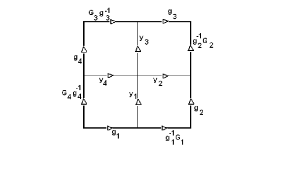
Figure 1: Subdivision of one plaquette

If there is a choice of densities $p\left(\cdot\right)$ that fulfill the consistency condition in this case, then it can be satisfied for whole directed set. For this case the consistency condition is simply

$$\frac{1}{Z^{{}^{\prime}}}\int p^{\prime}\left(g_{1}^{-1}G_{1}g_{2}y_{2}^{-1}y_{1}^{-1}\right)p^{\prime}\left(y_{2}g_{2}^{-1}G_{2}g_{3}^{-1}y_{3}^{-1}\right)p^{\prime}\left(y_{4}y_{3}g_{3}G_{3}^{-1}g_{4}^{-1}\right)p^{\prime}\left(g_{1}y_{1}y_{4}^{-1}g_{4}G_{4}^{-1}\right)$$ (38)

$$\prod_{i=1}^{4}d\mu_{H}\left(g_{i}\right)d\mu_{H}\left(y_{i}\right)d\mu_{H}\left(G_{i}\right)$$

$$= \frac{1}{Z}\int p\left(G_{1}G_{2}G_{3}^{-1}G_{4}^{-1}\right)\prod_{i=1}^{4}d\mu_{H}\left(G_{i}\right)$$

because integration over all the other plaquettes is the same in $\Gamma$ and $\Gamma^{{}^{\prime}}$. $p^{\prime}$ and $p$ denote the densities for plaquettes of size $\frac{a}{2^{k}}$ and $\frac{a}{2^{k-1}}$, respectively.

Using centrality of $p^{\prime}$, redefining

$$g_{1}y_{1}=X_{1},\qquad g_{2}y_{2}^{-1}=X_{2},\qquad y_{3}g_{3}=X_{3}^{-1},\qquad y_{4}^{-1}g_{4}=X_{4}^{-1}$$ (39)

and using invariance of the normalized Haar measure, one may integrate over $y_{1},y_{2},y_{3},y_{4}$ obtaining for the left hand side of (38)

$$\frac{1}{Z^{{}^{\prime}}}\int p^{\prime}\left(X_{1}^{-1}G_{1}X_{2}\right)p^{\prime}\left(X_{2}^{-1}G_{2}X_{3}\right)p^{\prime}\left(X_{3}^{-1}G_{3}^{-1}X_{4}\right)p^{\prime}\left(X_{4}^{-1}G_{4}^{-1}X_{1}\right)\prod_{i=1}^{4}d\mu_{H}\left(X_{i}\right)d\mu_{H}\left(G_{i}\right)$$

Finally, if there is a sequence of central functions $p^{\prime},p^{\prime\prime},p$ satisfying

$$\int p^{\prime}\left(G_{i}X\right)p^{\prime}\left(X^{-1}G_{j}\right)d\mu_{H}\left(X\right) \sim p^{\prime\prime}\left(G_{i}G_{j}\right)$$

$$\int p^{\prime\prime}\left(G_{i}X\right)p^{\prime\prime}\left(X^{-1}G_{j}\right)d\mu_{H}\left(X\right) \sim p\left(G_{i}G_{j}\right)$$ (40)

the consistency condition (38) would be satisfied, the proportionality constants being absorbed by the normalization constant $Z^{{}^{\prime}}$. $p^{\prime},p^{\prime\prime}$ and $p$ are the functions associated to the square plaquette with links of size $\frac{a}{2^{k}}$, the rectangular plaquette with links of size $\frac{a}{2^{k}}$ and $\frac{a}{2^{k-1}}$ and, finally, the square plaquette with links of size $\frac{a}{2^{k-1}}$. The sequence $\left(p^{\prime},p^{\prime\prime},p\right)$ corresponds to the subdivision of one plaquette. If such a sequence exists for all $k$, because all elements in the directed set $\left\{\Gamma,\succ\right\}$ may be reached by one-plaquette subdivisions, one obtains the following general result:

Theorem 1

An interaction measure on the projective limit $\mathcal{A}=\underset{\longleftarrow}{\lim}\mathcal{A}_{\Gamma}$ exists if a sequence of functions is found satisfying (40) for plaquette subdivisions of all sizes.

Notice that:

- Eq.(40) is not necessarily a convolution semigroup property because $p^{\prime},p^{\prime\prime}$ and $p$ might be different functions and (40) is a proportionality relation, not an equality.

- The interaction measure may not be absolutely continuous with respect to the kinematical measure $\nu$, constructed in Sect.2, because not all functions in the sequence (mostly in the small scale limit) might be continuous functions.

Although (40) is not exactly a convolution semigroup property, functions satisfying this condition may be obtained out of convolution semigroup kernels. Three cases will be separately analyzed, namely $G=U\left(1\right),SU\left(2\right),SU\left(3\right)$.

4.1 $G=U\left(1\right)$

An important convolution semigroup in $U\left(1\right)$

$$U\left(1\right)=\left\{e^{i2\pi\theta};\theta\in\left[0,1\right)\right\}$$ (41)

is the heat kernel semigroup

$$K_{1}\left(e^{i2\pi\theta},\beta\right)=\sum_{n\in\mathbb{Z}}\exp\left\{i2\pi n\theta-\left(2\pi n\right)^{2}\beta\right\}$$ (42)

which, by convolution with any initial condition $u_{0}\left(\theta\right)$, provides a solution to the $U\left(1\right)-$heat equation

$$\left(\frac{\partial}{\partial\beta}-\frac{\partial^{2}}{\partial\theta^{2}}\right)u\left(e^{i2\pi\theta},\beta\right)=0$$ (43)

Let us now use the $U\left(1\right)-$heat kernel in (42) with

$$p\left(e^{i2\pi\theta}\right)=K_{1}\left(e^{i2\pi\theta},\beta\right)$$ (44)

to check the condition (40). One obtains

$$\int K_{1}\left(e^{i2\pi\left(\theta_{1}+\alpha\right)},\beta^{\prime}\right)K_{1}\left(e^{i2\pi\left(\theta_{2}-\alpha\right)},\beta^{\prime}\right)d\alpha=K_{1}\left(e^{i2\pi\left(\theta_{1}+\theta_{2}\right)},2\beta^{\prime}\right)$$ (45)

Iterating this relation, one concludes that the measure consistency condition is satisfied with the choice (44) if

$$\beta^{\prime}=\frac{\beta}{4}$$ (46)

that is, each time one plaquette is subdivided the “time” label $\beta$ in the densities associated to that plaquette should be divided by $4$. Therefore, using the heat kernel as the density of the measure, a consistent measure is constructed in the projective limit.

An important consideration in establishing measures for the gauge spaces is to check whether, in the small scales, these measures correspond (or not) to the measures used by physicists for the same phenomena. In the $U\left(1\right)$ case this is easily seen by rewriting the heat kernel using the Jacobi identity

$$K_{1}\left(e^{i2\pi\theta},\beta\right)=\frac{1}{\sqrt{4\pi\beta}}\sum_{n\in\mathbb{Z}}\exp\left\{-\frac{\left(\theta+n\right)^{2}}{4\beta}\right\}$$ (47)

Then, at very small scales $\beta$ becomes extremely small. Therefore in the sum of (47) only the $n=0$ and the $\theta\approx 0$ neighborhood contribute and, for the plaquette, one obtains a density proportional to

$$\exp\left\{-\frac{\left(\theta_{1}+\theta_{2}-\theta_{3}-\theta_{4}\right)^{2}}{4\beta}\right\}$$ (48)

which indeed corresponds to the usual (small scale) $U\left(1\right)-$measure.

In the lattice used to define the $\left\{\Gamma,\succ\right\}$ directed set when, in the lattice size $\frac{a}{2^{k}}$, $k\rightarrow\infty$ then $\beta\rightarrow 0$. In this limit the density (47) is no longer continuous, therefore, the interaction measure is not absolutely continuous with respect to the kinematical $\nu$ measure. Nevertheless the interaction measure has a generalized density in $\mathcal{H}^{\ast}\left(\mathcal{A}\right)$, the distribution space of the projective gauge triplet described before. Summarizing:

Theorem 2

Using the density (47) for each link-based loop, with $\beta_{k}=c\frac{1}{4^{k}}$  ($c$ an arbitrary constant) for each $\Gamma_{k}$ in the directed set, a consistent measure is shown to exist in the projective limit $\mathcal{A}=\underset{\longleftarrow}{\lim}\mathcal{A}_{\Gamma_{k}}$ of the $U\left(1\right)$ gauge theory. Furthermore, the measure coincides at small scales with the Gaussian measure (48). The measure in the projective limit is not absolutely continuous with respect to the kinematical measure, but it has a generalized density in $\mathcal{H}^{*}\left(\mathcal{A}\right)$.

In Fig.2 one plots the density (47) for $\theta\in\left[0,1\right]$ and $\beta\in\left[0.001,0.4\right]$. One sees that for small $\beta$ (small scales) the measure concentrates around $\theta=0$.

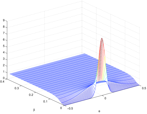
Figure 2: The $U\left(1\right)-$heat kernel density

4.2 Non-abelian compact groups

Now that the $U\left(1\right)$ case is understood, a simple argument shows that a similar construction is possible for general compact groups. In a compact Lie group the heat kernel is

$$K\left(g,\beta\right)=\sum_{\lambda\in\Lambda^{+}}d_{\lambda}e^{-c\left(\lambda\right)\beta}\chi_{\lambda}\left(g\right)$$ (49)

with $g\in G$ and $\beta\in\mathbb{R}^{+}$. $\Lambda^{+}$ is the set of highest weights, $d_{\lambda}$ and $\chi_{\lambda}\left(\cdot\right)$ the dimension and the character of the $\lambda-$representation and $c\left(\lambda\right)$ the spectrum of the Laplacian (10)

$$\left(\Delta_{G}\chi_{\lambda}\right)\left(g\right)=c\left(\lambda\right)\chi_{\lambda}\left(g\right)$$ (50)

Using, as before, the heat kernel for the construction of the interaction measure, the condition (40) becomes

$$\int d\mu_{H}\left(x\right)K\left(g_{1}x,\beta\right)K\left(x^{-1}g_{2},\beta\right)$$ (51)

$$= \sum_{\lambda,\lambda^{\prime}\in\Lambda^{+}}d_{\lambda}d_{\lambda^{\prime}}e^{-c\left(\lambda\right)\beta}e^{-c\left(\lambda^{\prime}\right)\beta}\int d\mu_{H}\left(x\right)\chi_{\lambda}\left(g_{1}x\right)\chi_{\lambda^{\prime}}\left(x^{-1}g_{2}\right)$$

$$= K\left(g_{1}g_{2},2\beta\right)$$

the last equality following from Schur’s orthogonality relations. Therefore, whenever the heat kernel is chosen as the density for the loops, the situation is quite similar to the $U\left(1\right)$ case, namely, on each subdivision of a plaquette

$$\beta\rightarrow\beta^{\prime}=\frac{\beta}{4}$$ (52)

Hence

Theorem 3

Using the heat kernel (49) for the density of each plaquette, with $\beta_{k}=c\frac{1}{4^{k}}$  ($c$ an arbitrary constant) for each $\Gamma_{k}$ in the directed set, a consistent measure is shown to exist in the projective limit $\mathcal{A}=\underset{\longleftarrow}{\lim}\mathcal{A}_{\Gamma_{k}}$ of the gauge theory with compact structure group $G$.

Notice that in the verification of the condition (40) by (51) what is important is the characters orthogonality relation. Therefore a different set of $c\left(\lambda\right)$’s might be used. This would lead to a different measure. The choice of which measure to choose would depend on physical considerations in the small scale limit.

The $SU\left(2\right)$ and $SU\left(3\right)$ cases will now be analyzed in detail

4.2.1 $SU\left(2\right)$

Here

$$\Lambda^{+} = \left\{\lambda:2\lambda\in\mathbb{N},\lambda\geq 0\right\}$$

$$c\left(\lambda\right) = \frac{1}{2}\lambda\left(\lambda+1\right)$$

$$d_{\lambda} = 2\lambda+1$$ (53)

$$K_{2}\left(g,\beta\right)=\sum_{\lambda\in\Lambda^{+}}\left(2\lambda+1\right)e^{-\frac{1}{2}\lambda\left(\lambda+1\right)\beta}\frac{\sin\left\{\left(2\lambda+1\right)\pi x\left(g\right)\right\}}{\sin\left\{\pi x\left(g\right)\right\}}$$ (54)

where $\pi x\left(g\right)$ is the angle coordinate of $g$ in a maximal torus. It may be obtained from the $2\times 2$ matrix representation of $g$ by

$$\pi x\left(g\right)=\cos^{-1}\left(\frac{Tr\left(g\right)}{2}\right)$$ (55)

$K_{2}\left(g,\beta\right)$ may be rewritten as

$$K_{2}\left(g,\beta\right)=2\left(2\pi\right)^{3/2}\frac{e^{\beta/8}}{\beta^{3/2}}\sum_{n\in\mathbb{Z}}\frac{x\left(g\right)+2n}{\sin\left\{\pi x\left(g\right)\right\}}\exp\left\{-2\pi^{2}\frac{\left(x\left(g\right)+2n\right)^{2}}{\beta}\right\}$$ (56)

One also sees that for small $\beta$ (small scales) the heat kernel density is dominated by the $n=0$ term in the sum above and by field configurations near $x\left(g\right)=0$. As in the $U\left(1\right)$ case, at $\beta=0$ the “densities” are no longer continuous functions and the measure in the projective limit space is not absolutely continuous with respect to the kinematical measure. There is however a generalized density in $\mathcal{H}^{\ast}\left(\mathcal{A}\right)$.

The structure of the measure at small scales may now be compared with the naive continuum limit of lattice theory, as discussed for example in [14]. There

$$U=e^{icaA_{\mu}^{b}\tau_{b}}$$ (57)

$c$ is a coupling constant, $a$ the lattice spacing, $A_{\mu}^{b}$ the continuum gauge field and $\tau_{b}$ a Lie algebra basis. Then, for a plaquette in the $1,2$ plane

$$U_{\square}\left(A\right)=e^{icaA_{1}^{b}\left(x_{\mu}-\frac{1}{2}a\delta_{\mu 2}\right)\tau_{b}}e^{icaA_{2}^{b}\tau_{b}\left(x_{\mu}+\frac{1}{2}a\delta_{\mu 1}\right)}e^{-icaA_{1}^{b}\left(x_{\mu}+\frac{1}{2}a\delta_{\mu 2}\right)\tau_{b}}e^{-icaA_{2}^{b}\left(x_{\mu}-\frac{1}{2}a\delta_{\mu 1}\right)\tau_{b}}$$ (58)

which for small $a$ leads to

$$Tr\left(U_{\square}\left(A\right)\right)\simeq 2-\frac{c^{2}a^{4}}{4}F_{12}^{b}F_{12}^{b}$$ (59)

On the other hand, from (55), one knows that

$$TrU_{\square}=2\cos\left(\pi x\left(U_{\square}\right)\right)$$

or $TrU_{\square}\simeq 2\left(1-\frac{1}{2}\pi^{2}x^{2}\left(U_{\square}\right)\right)$ for small $x$. Comparing with (59) one concludes that

$$x^{2}\left(U_{\square}\right)=\frac{c^{2}a^{4}}{4\pi^{2}}F_{12}^{b}F_{12}^{b}$$

Therefore, for small $\beta$, the measure that uses (56) as its density coincides with the usual physical continuum measure.

In Fig.3 one plots the density (56) for different values of $\theta=\pi x$ and $\beta$. As in the $U\left(1\right)$ case, one sees that for small $\beta$ (small scales) the measure concentrates around $\theta=0$.

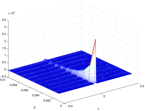
Figure 3: The $SU\left(2\right)-$ heat kernel density

4.2.2 $SU\left(3\right)$

The irreducible representations of $SU\left(3\right)$ are labelled by two positive integers $\left(p,q\right)$ ($\left(1,1\right)$ is the one-dimensional representation, $\left(2,1\right)=\underset{\backsim}{3},\left(1,2\right)=\underset{\backsim}{3}^{\ast}$, etc.). The eigenvalues of the Laplacian and dimensions of the representations are

$$c\left(p,q\right) = \frac{1}{3}\left(p^{2}+q^{2}+pq\right)-1$$

$$d_{p,q} = \frac{1}{2}pq\left(p+q\right)\hskip 28.45274ptp,q=1,2,\cdots$$ (60)

With $\left(\theta_{1}\left(g\right),\theta_{2}\left(g\right)\right)$ denoting the angle coordinates of $g$ in the maximal torus $diag\left\{\exp\left(i\theta_{1}\right),\exp\left(i\theta_{2}\right),\exp\left(-i\left(\theta_{1}+\theta_{2}\right)\right)\right\}$, obtained from

$$\cos\theta_{1}\left(g\right)+\cos\theta_{2}\left(g\right)+\cos\left(\theta_{1}-\theta_{2}\right)\left(g\right) = \textnormal{Re}Tr\left(g\right)$$

$$\sin\theta_{1}\left(g\right)+\sin\theta_{2}\left(g\right)-\sin\left(\theta_{1}-\theta_{2}\right)\left(g\right) = \textnormal{Im}Tr\left(g\right)$$ (61)

the $SU\left(3\right)$ heat kernel is [15]

$$K_{3}\left(g,\beta\right)$$

$$= \frac{1}{s\left(\theta_{1},\theta_{2}\right)}\sum_{l=-\infty}^{\infty}\sum_{m=-\infty}^{\infty}\left\{\theta_{1}-\theta_{2}+2\pi\left(l-m\right)\right\}\left\{\theta_{1}+2\theta_{2}+2\pi\left(l+2m\right)\right\}\times$$

$$\left\{2\theta_{1}+\theta_{2}+2\pi\left(2l+m\right)\right\}\exp\left\{-\frac{1}{2\beta}\left[\left(\theta_{1}+2\pi l\right)^{2}+\left(\theta_{2}+2\pi m\right)^{2}+\left(\theta_{1}+2\pi l\right)\left(\theta_{2}+2\pi m\right)\right]\right\}$$

with

$$s\left(\theta_{1},\theta_{2}\right)=8\sin\frac{1}{2}\left(\theta_{1}-\theta_{2}\right)\sin\frac{1}{2}\left(2\theta_{1}+\theta_{2}\right)\sin\frac{1}{2}\left(\theta_{1}+2\theta_{2}\right)$$ (63)

That the choice $p\left(g\right)=K_{3}\left(g,\beta\right)$ and $p^{\prime}\left(g\right)=K_{3}\left(g,\frac{\beta}{4}\right)$, for each plaquette subdivision, satisfies the consistency condition (40) follows from the general result (Theorem 3).

Now one checks the consistency of the result with the physical small scale (small $\beta$) limit. Inspection of (LABEL:5.30) leads to the conclusion that for $\beta=0$ the sums become dominated by the $l=m=0$ term and the neighborhood $\left(\theta_{1}\thickapprox 0,\theta_{2}\thickapprox 0\right)$. Then

$$K_{3}\left(g,\beta\right)\underset{\beta\rightarrow 0}{\longrightarrow}\exp\left\{-\frac{1}{2\beta}\left(\theta_{1}^{2}+\theta_{2}^{2}+\theta_{1}\theta_{2}\right)\right\}$$

From (61) one also sees that for small $\theta_{1},\theta_{2}$

$$3-\theta_{1}^{2}-\theta_{2}^{2}-\theta_{1}\theta_{2}\backsimeq Tr\left(g\right)$$

which, equating with (59), leads to

$$\theta_{1}^{2}+\theta_{2}^{2}+\theta_{1}\theta_{2}\backsimeq 1-\frac{c^{2}a^{4}}{4}F_{12}^{b}F_{12}^{b}$$

That is, up to an irrelevant constant factor (to be absorbed in the measure normalization), one also obtains in the $SU(3)$ case the usual physical measure in the $\beta\rightarrow 0$ limit. Therefore, both for $SU\left(2\right)$ and $SU\left(3\right)$, one may take the measures so constructed as a definition of the Yang-Mills measure.

For small $\beta$ the measure is always concentrated in the neighborhood $\left(\theta_{1}\thickapprox 0,\theta_{2}\thickapprox 0\right)$.

5 Gauge measure and the strata

Let $S_{A}$ be the stabilizer (isotropy group) of a generalized connection $A\in\mathcal{A}$

$$S_{A}=\left\{\gamma\in\mathcal{G}:\gamma A=A\right\}$$ (64)

The action of the gauge group $\mathcal{G}$ on $\mathcal{A}$ leads to a stratification of $\mathcal{A}$ corresponding to the classes of equivalent orbits $\left\{gA;g\in\mathcal{G}\right\}$. The stratum $\Sigma\left(A\right)$ of $A$ is the set of connections having isotropy groups $\mathcal{G}-$conjugated to that of $A$

$$\Sigma\left(A\right)=\left\{B\in\mathcal{A}:\exists\gamma\in\mathcal{G}:S_{B}=\gamma S_{A}\gamma^{-1}\right\}$$ (65)

The configuration space of the gauge theory is the quotient space $\mathcal{A}/\mathcal{G}$ and therefore a stratum is the set of points in $\mathcal{A}/\mathcal{G}$ that correspond to orbits with conjugated isotropy groups.

When $G$ is a compact group the stratification is topologically regular. The map that, to each orbit, assigns the conjugacy class of its isotropy group is called the type. The set of strata carries a partial ordering of types, $\Sigma_{\tau}\subseteq\Sigma_{\tau^{{}^{\prime}}}$ with $\tau\leq\tau^{\prime}$ if there are representatives $S_{\tau}$ and $S_{\tau^{\prime}}$ of the isotropy groups such that $S_{\tau}\supseteq S_{\tau^{\prime}}$. The maximal element in the ordering of types is the class of the center $Z(G)$ of $G$ and the minimal one is the class of $G$ itself. Furthermore $\cup_{t\geq\tau}\Sigma_{t}$ is open and $\Sigma_{\tau}$ is open in the relative topology in $\cup_{t\leq\tau}\Sigma_{t}$.

Because the isotropy group of a connection is isomorphic to the centralizer of its holonomy group, the strata are in one-to-one correspondence with the Howe subgroups of $G$, that is, the subgroups that are centralizers of some subset in $G$. Given an holonomy group $H_{\tau}$ associated to a connection $A$ of type $\tau$, the stratum of $A$ is classified by the conjugacy class of the isotropy group $S_{\tau}$, that is, the centralizer of $H_{\tau}$

$$S_{\tau}=Z\left(H_{\tau}\right)$$ (66)

An important role is also played by the centralizer of the centralizer

$$H_{\tau}^{\prime}=Z\left(Z\left(H_{\tau}\right)\right)$$ (67)

that contains $H_{\tau}$ itself. If $H_{\tau}^{\prime}$ is a proper subgroup of $G$, the connection $A$ reduces locally to the subbundle $P_{\tau}=\left(M,H_{\tau}^{\prime}\right)$. Global reduction depends on the topology of $M$, but it is always possible if $P$ is a trivial bundle. $H_{\tau}^{\prime}$ is the structure group of the maximal subbundle associated to type $\tau$. Therefore the types of strata are also in correspondence with types of reductions of the connections to subbundles. If $S_{\tau}$ is the center of $G$ the connection is called irreducible, all others are called reducible. The stratum of the irreducible connections is called the generic stratum.

Now, for $G=SU\left(2\right)$ and $SU\left(3\right)$ one describes the strata and how they stand in relation to the measures defined before. In $G=SU(2)$, the isotropy groups (equivalently, the centralizers of the holonomy) and the structure groups of the maximal subbundles are :

$$S_{A}$$

1

2

3

(68)

There are three strata. Stratum 1 is the generic stratum. The other two are reducible strata.

A $SU\left(2\right)$ transformation may be parametrized by

$$\exp\left(-i\frac{\theta}{2}\overset{\rightarrow}{n}\cdot\overset{\rightarrow}{\sigma}\right)=\boldsymbol{1}\cos\frac{\theta}{2}+i\left(\overset{\rightarrow}{n}\cdot\overset{\rightarrow}{\sigma}\right)\sin\frac{\theta}{2}$$ (69)

Geometrically, the $SU\left(2\right)$ group may be pictured as a sphere of radius $4\pi$, with all the points at radial distance $2\pi$ identified to $\left(\begin{array}[]{cc}-1&0\\ 0&-1\end{array}\right)$ and the points at radius $4\pi$ identified with the center of the sphere. The reducible stratum 3 corresponds to a $\mathbb{Z}_{2}-$bundle, that is, to homomorphisms of the loops to a two point space $\left(\theta=0,\theta=2\pi\right)$. Each reducible stratum of type 2 is a $U\left(1\right)-$bundle corresponding to homorphisms of the loops to the $SU\left(2\right)$ transformations along one radius (fixed $\overset{\rightarrow}{n}$, variable $\theta$). Because adjoint transformations transform any radius into any other, all $U\left(1\right)-$bundles are equivalent and represent the same gauge configurations. Finally, the (generic) stratum 1 corresponds to homomorphisms to arbitrary $SU\left(2\right)$ transformations.

From (55) one sees that the intensity of the measure (54) only depends on the first term $\boldsymbol{1}\cos\frac{\theta}{2}$ in the parameterization (69). Therefore all strata approach the small $x\left(g\right)$ region where the measure is peaked and therefore they all are expected to be relevant in the physical behavior of the gauge theory.

For $G=SU(3)$ the isotropy groups and the structure groups of the maximal subbundles are :

$$S_{A}$$

1

2

3

4

5

(70)

There are five strata. Stratum 1 is the generic stratum. All others are reducible strata. To find out their relevance in the framework of the measure (LABEL:5.30) one uses the following parametrization [16] for an arbitrary $SU\left(3\right)$ transformation,

$$U=u_{0}+iu_{k}\lambda_{k}$$ (71)

where $u_{k}=\alpha a_{k}+\beta d_{ijk}a_{i}a_{j}$ for an octet vector $a_{k}$, with $u_{0},\alpha$ and $\beta$ being functions of the invariants

$$\begin{array}[]{lll}I_{2}\left(a\right)&=&a_{i}a_{i}\\ I_{3}\left(a\right)&=&d_{ijk}a_{i}a_{j}a_{k}\end{array}$$ (72)

which can be built from the vector $a_{k}$. Then

$$\begin{array}[]{lll}u_{0}&=&\frac{1}{3}\sum_{n}e^{i\varphi_{n}}\\ \alpha&=&-\sum_{n}\varphi_{n}e^{i\varphi_{n}}\left(3\varphi_{n}^{2}-I_{2}\right)^{-1}\\ \beta&=&-\sum_{n}e^{i\varphi_{n}}\left(3\varphi_{n}^{2}-I_{2}\right)^{-1}\end{array}$$ (73)

with

$$\varphi_{n}=2\left(\frac{I_{2}}{3}\right)^{\frac{1}{2}}\cos\frac{1}{3}\left(2\pi n+\cos^{-1}\left(\sqrt{3}I_{3}I_{2}^{-\frac{3}{2}}\right)\right);\hskip 12.80365ptn=1,2,3$$ (74)

As before, one sees from (61) that the intensity of the measure only depends on $\textnormal{Re}u_{0}$ and $\textnormal{Im}u_{0}$, whereas the choice of the subbundle for each stratum depends on the choice of the $u_{k}$ coefficients. Therefore there is for all strata a range of parameters that approaches the region where the measure is peaked.

6 Remarks and conclusions

1) The Cartesian product point of view, in the construction of the projective limit $\mathcal{A}=\underset{\longleftarrow}{\lim}\mathcal{A}_{\Gamma}$ and of the triplet $\mathcal{H}\left(\mathcal{A}\right)\subset L^{2}\left(\mathcal{A},d\nu\right)\mathcal{\subset H}^{\ast}\left(\mathcal{A}\right)$, means that a consistent framework is obtained for the description of gauge theories at all length scales. In this setting the lattice structure, underlying the Cartesian product, is not an approximation scheme but a framework to characterize the theory at the several length scales.

2) For each $\mathcal{A}_{\Gamma}=Hom\left(E\left(\Gamma\right),G\right)\sim G^{\#E\left(\Gamma\right)}$, the interaction measure $\frac{1}{Z}p\left(\mathcal{A}_{\Gamma}\right)\left(d\mu_{H}\right)^{\#E\left(\Gamma\right)}$, constructed in Section 4 is absolutely continuous with respect the kinematical measure. However when $\beta\rightarrow 0$ the ”density” ceases to be a continuous function. Therefore, for the full projective limit, the interaction measure is not absolutely continuous with respect to the kinematical measure. That such a result was to be expected, follows also from the analysis of Fleischhak [17] [18] who, starting from very general conditions concluded that in gauge theories there is a ”breakdown of the action method”. However, in the gauge triplet framework, one may consider that a generalized density exists in $\mathcal{H}^{\ast}\left(\mathcal{A}\right)$.

3) The fact that the small $\beta$ component of the interaction measures coincides with the usual small distance representations of the abelian and the Yang-Mills measure, mean that they will inherit the same qualitative physical properties. In particular, the absence of a mass gap in the abelian case and, for the non-abelian case, the same qualitative properties as obtained, for example, from asymptotic dynamics [19], namely the fact that either there is spontaneous violation of the symmetry or all asymptotic states are color singlets.

4) As to the role of non-generic strata in gauge theories, the fact that there is for all strata a range of parameters that approaches the region where the measure is peaked, emphasizes the importance of these strata for the structure of low-lying excitations. A similar result [20] had been obtained using a ground-state approximation [21] [22] for the non-abelian ground-state.

References

• [1] A. Ashtekar and C. J. Isham; Representations of the holonomy algebras of gravity and nonabelian gauge theories, Class. Quant. Grav. 9 (1992) 1433-1468.
• [2] A. Ashtekar and J. Lewandowski; Differential geometry on the space of connections via graphs and projective limits, J. Geom. Phys. 17 (1995) 191-230.
• [3] A. Ashtekar and J. Lewandowski; Projective techniques and functional integration for gauge theories, J.Math. Phys. 36 (1995) 2170-2191.
• [4] D. Marolf and J. M. Mourão; On the support of the Ashtekar-Lewandowski measure, Commun. Math. Phys. 170 (1995) 583-606.
• [5] A. Ashtekar and J. Lewandowski; Representation theory of analytic holonomy C algebras, (arXiv:gr-qc/9311010) in Knots and Quantum Gravity (J. Baez, Ed.) Oxford Univ. Press, Oxford 1994.
• [6] J. Baez and S. Sawin; Functional integration on spaces of connections, J. Funct. Anal. 150 (1997) 1-26.
• [7] C. Fleischhack; Stratification of the generalized gauge orbit space, Comm. Math. Phys. 214 (2000) 607-649.
• [8] C. Fleischhack; On the Structure of Physical Measures in Gauge Theories, arXiv:math-ph/0107022.
• [9] C. Fleischhack; Hyphs and the Ashtekar-Lewandowski measure, J. Geom. Phys. 45 (2003) 231-251.
• [10] J. Kisynski; On the generation of tight measures, Studia Math. 30 (1968) 141-151.
• [11] K. Maurin; General eigenfunction expansions and unitary representations of topological groups, PWN - Polish Scient. Publ., Warszawa 1968.
• [12] T. Deck; Hida distributions on compact Lie groups, Inf. Dim. Anal., Quantum Prob. and Rel. Topics 3 (2000) 337-362.
• [13] I. M. Gelfand and G. E. Shilov; Generalized functions, vol.2, Academic Press, NY 1968.
• [14] M. Creutz; Quarks, gluons and lattices, Cambridge U. P., Cambridge 1983.
• [15] B. E. Baaquie; Character functions of SU(3), J. Phys. A: Math. Gen. 21 (1988) 2651-2656.
• [16] A. J. Macfarlane, A. Sudbery and P. H. Weisz; On Gell-Mann’s $\lambda$-matrices, d- and f-tensors, octets and parametrization of SU(3), Commun. Math. Phys. 11 (1968) 77-90.
• [17] C. Fleischhack; On the structure of physical measures in gauge theories, arXiv:math-ph/0107022.
• [18] C. Fleischhack; On the support of physical measures in gauge theories, arXiv:math-ph/0109030.
• [19] R. Vilela Mendes; Asymptotic dynamics for gauge theories, Phys. Rev. D18 (1978) 4726-4736.
• [20] R. Vilela Mendes; Stratification of the orbit space in gauge theories. The role of nongeneric strata, J. Phys. A: Math. Gen. 37 (2004) 11485-11498.
• [21] R. Vilela Mendes; Stochastic processes and the non-perturbative structure of the QCD vacuum, Z. Phys. C - Particles and Fields 54 (1992) 273-281.
• [22] R. Vilela Mendes; Path-integral estimates of ground-state functionals, Proceedings of the International Conference on Mathematical Analysis of Random Phenomena, pags. 169-177, World Scientific 2006.