A renormalized large-$n$ solution
of the $U(n)\times U(n)$ linear sigma model
in the broken symmetry phase

Abstract

Dyson-Schwinger equations for the $U(n)\times U(n)$ symmetric matrix sigma model reformulated with two auxiliary fields in a background breaking the symmetry to $U(n)$ are studied in the so-called bare vertex approximation. A large $n$ solution is constructed under the supplementary assumption so that the scalar components are much heavier than the pseudoscalars. The renormalizability of the solution is investigated by explicit construction of the counterterms.

I Introduction

Universal features of finite temperature and finite density variation of the QCD ground state realizing the $SU(3)_{R}\times SU(3)_{L}$ approximate chiral symmetry were understood with the help of the corresponding meson model pisarski84 . There were also numerous attempts to treat quantitatively the finite temperature restoration of chiral symmetry of the strongly interacting matter in the framework of this model. A common goal of these investigations is the description of the quark mass dependence of the nature of the finite temperature symmetry restoration lenaghan00 ; roder03 ; herpay05 . Another central issue is the nature of the phase transition, when the baryonic density is varied. For its investigation one couples constituent quarks carrying baryon number to the meson model bilic98 ; kovacs09 ; schaefer09 ; schaefer10 .

Optimistically one could say, that the location of the characteristic points of the QCD phase diagram determined with different variants of the model and in different approximations do agree with each other and with the results of the lattice field theoretical simulations within a factor of 2. In particular, improved agreement with lattice determinations of the QCD phase diagram were reported, when the Polyakov loop degree of freedom is coupled to the quark-meson model kahana08 ; mao10 ; gupta10 . But the effective models are all strongly coupled, therefore one usually experiences large variations in their predictions, when the simplest mean-field treatments are improved by taking into account quantum fluctuations of the mesons and the constituent quarks marko10 ; herbst10 . This circumstance limits the competitivity of their predictions.

Some time ago we initiated the application of the expansion in the number of quark flavors for the description of the chiral symmetry restoration in the two-flavor model patkos02 ; jakovac04 . The approach was suggested by the $SU(2)\times SU(2)\sim O(4)$ isomorphy and the fortunate fact that the $N=\infty$ solution of the $O(N)$ model is the textbook example of the application of the $1/N$ expansion zinn-justin02 . Recently, next-to-leading order (NLO) results were also presented for the pressure of the relativistic $O(N)$ model and applied to the physical ($N=4$) sigma-pion gas andersen04 ; andersen08 . In this context also the renormalizability of the NLO approximation was fully clarified and shown to be valid in various formulations of the model (with and without auxiliary field) fejos09 .

An analogous development for the three-flavor meson (and quark-meson) model is hindered, because even the leading order solution of the large-$n$ limit of the $U(n)\times U(n)$ symmetric linear sigma-model is unknown. Progress would represent interest also for the Higgs sector of technicolor models of electroweak symmetry breaking appelquist95 ; kikukawa07 . To our best knowledge, no published attempts exist, which would go beyond the partial large-$n$ treatments of the $O(2n^{2})$-symmetric nonlinearities. The results obtained with such an approach are questionable in light of the rather different finite temperature renormalization group behavior of the $O(2n^{2})$ and $U(n)\times U(n)$ symmetric models for $n\geq 3$ pisarski84 ; paterson81 .

The goal of the present paper is to describe an approximate leading order ($n=\infty$) solution. Although it takes into account only two-loop contributions to the 2PI (two-particle irreducible) effective action, it definitely goes beyond the $O(2n^{2})$ symmetric solution. It exploits in addition to the large $n$ expansion an assumption concerning the mass spectra of the model. The region in the coupling space, where this assumption is valid can be estimated by determining the spectra from the approximate solution self-consistently. In this paper we present the construction of the renormalized version of this solution in some detail, and provide also an illustrative investigation of its range of validity. A deeper analysis of the mass spectra and the finite temperature features are left to a forthcoming publication.

The idea to impose an extra assumption on the mass spectra stems from the common practice of dealing with the 4 scalars and 4 pseudoscalars defining the $SU(2)\times SU(2)$ symmetric meson model. One simply omits half of the fields, e.g. the 3 components of the scalar-isovector triplet and the pseudoscalar-isoscalar singlet with reference to their higher mass. One arrives this way at the Gell-Mann–Lévy linear sigma model. We shall assume an analogous feature to occur in the spectra of the leading order solution at large $n$. We do not attempt the anomalous realization of the $U_{A}(1)$ symmetry, therefore in this limiting case all pseudoscalars will have the same mass. Based on this assumption, in a first approximation to the $n=\infty$ solution we retain only the quantum fluctuations of the light pion fields. After finding the propagators of the scalar fields, one calculates corrections to the pion propagator arising from the heavy scalar fluctuations. In principle, one can iterate this procedure until the solution of the large-$n$ bare vertex approximation (BVA) is reached. It will be demonstrated, that the pion fields still obey Goldstone’s theorem after the scalar corrections are included. We shall explore the divergence structure of the equation of state, the pion self-energy and the saddle-point equations (SPEs), and determine the counterterm pieces in the effective action necessary for their renormalization.

The paper is organized as follows. In Sec. II, the model is reformulated with two auxiliary fields. We elaborate also on the expected mixing structure of the solution. In Sec. III, the leading large-$n$ Dyson-Schwinger (DS) equations are presented in BVA and the corresponding 2PI effective potential is constructed. In Sec. IV, we present an approximate solution, which is valid when the scalars are much heavier than the pseudoscalar fields of the model. Here also a simplified exploration of the range of validity of this assumption is given. The renormalizability of the proposed solution is investigated in Sec. V. In the divergence analysis we rely on a number of cutoff sensitive integrals collected in Appendix A. The paper ends with the conclusions (Sec. VI).

II Formulation of the model with auxiliary fields

The Lagrangian of the model in its usual form reads as

$$L=\textrm{Tr}[\partial_{\mu}M\partial^{\mu}M^{\dagger}-m^{2}MM^{\dagger}]-\frac{g_{1}}{n^{2}}(\textrm{Tr}MM^{\dagger})^{2}-\frac{g_{2}}{n}\textrm{Tr}(MM^{\dagger})^{2}+\sqrt{2n^{2}}hs^{0},$$ (1)

where the algebra valued complex field $M$ is parametrized with help of the generators of the $U(n)$ group:

$$M=(s^{a}+i\pi^{a})T^{a},\qquad{\textrm{Tr}}T^{a}T^{b}=\frac{1}{2}\delta^{ab},\qquad a=0,1,...,n^{2}-1.$$ (2)

In terms of the matrix elements, it can be written in the following form:

$$L = \frac{1}{2}[(\partial_{\mu}s^{a})^{2}+(\partial_{\mu}\pi^{a})^{2}-m^{2}((s^{a})^{2}+(\pi^{a})^{2})]+\sqrt{2n^{2}}hs^{0}$$ (3)

$$- \frac{g_{1}}{4n^{2}}\Big{(}(s^{a})^{2}+(\pi^{a})^{2}\Big{)}^{2}-\frac{g_{2}}{2n}(U^{a})^{2},$$

where the $U(n)$ vector $U^{a}$ is defined as

$$U^{a}=\frac{1}{2}d^{abc}(s^{b}s^{c}+\pi^{b}\pi^{c})-f^{abc}s^{b}\pi^{c},$$ (4)

with $d^{abc}$ and $f^{abc}$ being the symmetric and antisymmetric structure constants of the $U(n)$ group, respectively. Some useful relations involving them can be found in Appendix B., which are needed in order to obtain the subsequent equations. Two auxiliary fields are introduced by adding the following constraints to the Lagrangian:

$$\Delta L=-\frac{1}{2}\left(X-i\sqrt{\frac{g_{1}}{2n^{2}}}((s^{a})^{2}+(\pi^{a})^{2})\right)^{2}-\frac{1}{2}\left(Y^{a}-i\sqrt{\frac{g_{2}}{n}}U^{a}\right)^{2}.$$ (5)

In the sum ${\cal L}\equiv L+\Delta L$ the $U(n)\times U(n)\rightarrow U(n)$ symmetry breaking pattern corresponds to the shifts

$$s^{a}\rightarrow s^{a}+\sqrt{2n^{2}}v\delta^{a0},\qquad U^{a}\rightarrow U^{a}+2\sqrt{n}vs^{a}+n\sqrt{2n}\delta^{a0}v^{2}.$$ (6)

After the introduction of the auxiliary field variables and the shifts, the full Lagrangian has the following form:

$${\cal L} = \frac{1}{2}\Big{[}(\partial_{\mu}s^{a})^{2}+(\partial_{\mu}\pi^{a})^{2}-m^{2}\Big{(}2n^{2}v^{2}+2\sqrt{2n^{2}}vs^{0}+(s^{a})^{2}+(\pi^{a})^{2}\Big{)}\Big{]}+\sqrt{2n^{2}}h(s^{0}+\sqrt{2n^{2}}v)$$ (7)

$$- \frac{1}{2}X^{2}-\frac{1}{2}(Y^{a})^{2}+i\sqrt{\frac{g_{1}}{2n^{2}}}X\Big{(}2n^{2}v^{2}+2\sqrt{2n^{2}}vs^{0}+(s^{a})^{2}+(\pi^{a})^{2}\Big{)}$$

$$+ i\sqrt{\frac{g_{2}}{n}}Y^{a}(U^{a}+2\sqrt{n}vs^{a}+\sqrt{2n^{3}}\delta^{a0}v^{2}).$$

Next, we shortly describe the assumed structure of the solution and introduce some notations. The classical constraint equations show that the background $v$ induces nonzero $X,Y^{0}$ values and introduces mixing of the pair $s^{0},X$ and also of $s^{a},Y^{a}$ for every value of the index $a$. We construct correspondingly a quantum solution, where the saddle-point values of $X,Y^{0}$ are nonzero, $Y^{a}=0,a\neq 0$, and only the following 2-point functions do not vanish:

$$\displaystyle[G_{s^{0}X},\quad G_{s^{0}Y^{0}},\quad G_{XY^{0}},\quad G_{s^{0}s^{0}},\quad G_{Y^{0}Y^{0}},\quad G_{XX}],$$

$$\displaystyle[G_{s^{u}s^{v},u=v\neq 0},\quad G_{s^{u}Y^{v},u=v\neq 0},\quad G_{Y^{u}Y^{v},u=v\neq 0}],\qquad G_{\pi^{u}\pi^{v},u=v}.$$ (8)

The sets in square brackets form mixing sets of fields: there is a 3-dimensional mixing sector, and there are $n^{2}-1$ identical copies of 2-dimensional mixing two-point functions. The $\pi$ sector is diagonal. The equations presented in the next section show degeneracy of the 2-point functions for $u=v\neq 0$, therefore it is convenient to introduce the following short-hand notations:

$$\displaystyle G_{s^{0}s^{0}}\equiv G_{s^{0}},\quad G_{XX}\equiv G_{X},\quad G_{Y^{0}Y^{0}}\equiv G_{Y^{0}},\quad G_{\pi^{0}\pi^{0}}\equiv G_{\pi^{0}},$$

$$\displaystyle\quad G_{\pi^{u}\pi^{u}}\equiv G_{\pi},\quad G_{s^{u}s^{u}}\equiv G_{s},\quad G_{s^{u}Y^{u}}\equiv G_{sY},\quad G_{Y^{u}Y^{u}}\equiv G_{Y},\qquad u\neq 0.$$ (9)

III Dyson-Schwinger equations and their truncation

III.1 The equation of state and the saddle-point equations

Standard rules rivers of constructing the derivatives of the quantum effective action $\Gamma$ with respect to the fields leads to the following expressions:

$$\frac{\delta\Gamma}{\delta X} = -X+i\sqrt{\frac{g_{1}}{2n^{2}}}\Big{(}2n^{2}v^{2}+2\sqrt{2n^{2}}vs^{0}+(s^{a})^{2}+G_{s^{a}s^{a}}+(\pi^{a})^{2}+G_{\pi^{a}\pi^{a}}\Big{)},$$

$$\frac{\delta\Gamma}{\delta Y^{u}} = -Y^{u}+i\sqrt{\frac{g_{2}}{n}}\Big{(}U^{u}+2\sqrt{n}vs^{u}+\sqrt{2n^{3}}\delta^{u0}v^{2}+\frac{1}{2}d^{ubc}(G_{s^{b}s^{c}}+G_{\pi^{b}\pi^{c}})-f^{ubc}G_{s^{b}\pi^{c}}\Big{)},$$

$$\frac{\delta\Gamma}{\delta s^{u}} = -(\square+m^{2})s^{u}-\Big{(}m^{2}\sqrt{2n^{2}}-2i\sqrt{g_{1}}X\Big{)}v\delta^{u0}+\sqrt{2n^{2}}h\delta^{u0}+i\frac{\sqrt{2g_{1}}}{n}(Xs^{u}+G_{Xs^{u}})$$

$$+ i\sqrt{\frac{g_{2}}{n}}\Big{[}d^{abu}(s^{b}Y^{a}+G_{s^{b}Y^{a}})+2\sqrt{n}vY^{u}-f^{auc}(\pi^{c}Y^{a}+G_{\pi^{c}Y^{a}})\Big{]},$$

$$\frac{\delta\Gamma}{\delta\pi^{u}} = -(\square+m^{2})\pi^{u}+i\frac{\sqrt{2g_{1}}}{n}(X\pi^{u}+G_{X\pi^{u}})+i\sqrt{\frac{g_{2}}{n}}\Big{[}d^{abu}(\pi^{b}Y^{a}+G_{\pi^{b}Y^{a}})-f^{abu}(s^{b}Y^{a}+G_{s^{b}Y^{a}})\Big{]}.$$ (10)

Taking further functional derivatives of these expressions, one arrives at the equations of the 2-point functions (see next subsection). Also when one equates the derivatives of $\Gamma$ to zero, the equations determining the physical value of the background $v$ and the auxiliary fields $X,Y^{0}$ are obtained (we do not distinguish the notations of the solutions of these equations from the variables taking arbitrary values). Using the Fourier representation of the propagators, from (10) one gets the two SPEs and the equation of state (EoS) (setting $u=0$) at the leading order of the large $n$ expansion as

$$0 = -X+in\sqrt{2g_{1}}v^{2}+i\sqrt{\frac{g_{1}}{2}}n\left(\int_{k}G_{s}(k)+\int_{k}G_{\pi}(k)\right),$$

$$0 = -Y^{0}+in\sqrt{2g_{2}}v^{2}+i\sqrt{\frac{g_{2}}{2}}n\left(\int_{k}G_{s}(k)+\int_{k}G_{\pi}(k)\right),$$

$$0 = -\sqrt{2}nv\Big{(}m^{2}-i\frac{\sqrt{2g_{1}}}{n}X-i\frac{\sqrt{2g_{2}}}{n}Y^{0}\Big{)}+\sqrt{2}nh+i\sqrt{2g_{2}}n\int_{k}G_{sY}(k),$$ (11)

respectively. We note, that the equations for $\pi^{a}$ and $s^{u}$ imply for $u\neq 0$ vanishing expectation values automatically, taking into account the above assumed list of the nonvanishing 2-point functions. One should also note, that the auxiliary fields $X,Y^{0}\sim{\cal{O}}(n)$. Comparing the solutions of the equations for the two auxiliary fields, one finds a relation valid both in renormalized and unrenormalized versions:

$$\sqrt{g_{1}}Y^{0}=\sqrt{g_{2}}X.$$ (12)

Also, it proves useful in the further discussion to introduce the combination

$$M^{2}=m^{2}-\frac{i}{n}(\sqrt{2g_{1}}X+\sqrt{2g_{2}}Y^{0}).$$ (13)

III.2 The propagator equations

The second derivatives of the effective action yield the various 2-point functions. It is convenient to introduce the following tree-level inverse propagator commonly appearing in several two-point functions:

$$iD_{0}^{-1}(p)=p^{2}-M^{2}.$$ (14)

In this section we substitute for all 3-point functions their classical expressions listed below in (15) and therefore close the coupled set of DS equations at the 2-point level (BVA). From (7) one can read off the nonzero classical 3-point couplings:

$$\displaystyle\Gamma_{X\pi^{a}\pi^{b}}=\Gamma_{Xs^{a}s^{b}}=i\frac{\sqrt{2g_{1}}}{n}\delta^{ab}\delta(x-y)\delta(x-z),$$

$$\displaystyle\Gamma_{Y^{a}s^{b}s^{c}}=\Gamma_{Y^{a}\pi^{b}\pi^{c}}=i\sqrt{\frac{g_{2}}{n}}d^{abc}\delta(x-y)\delta(x-z),\qquad\Gamma_{Y^{a}s^{b}\pi^{c}}=-i\sqrt{\frac{g_{2}}{n}}f^{abc}\delta(x-y)\delta(x-z).$$ (15)

In the pseudoscalar sector the following DS-equations are found at leading order (the abbreviated notation $\int G_{[.]}G_{[.]}\equiv\int_{k}G_{[.]}(k)G_{[.]}(p+k)$ is used):

$$iG_{\pi^{0}}^{-1} = iD_{0}^{-1}-2ig_{2}\int G_{Y}G_{\pi},$$

$$iG_{\pi}^{-1} = iD_{0}^{-1}-ig_{2}\int G_{Y}(G_{s}+G_{\pi})+ig_{2}\int G_{sY}G_{sY}.$$ (16)

One notes the potential violation of Goldstone’s theorem when comparing $G_{\pi}(k=0)$ or $G_{\pi^{0}}(k=0)$ with the equation of state. Nevertheless, our approximate solution obeys this theorem due to a rather nontrivial relation between the relevant tadpole and bubble contributions (see next section). The previous relations also hint to a possible further dynamical violation of the remaining $U(n)$ symmetry to $SU(n)$ due to the coupling of the auxiliary variables $Y^{u}$ to the scalar fields $s^{u}$, which is proportional to the antisymmetric structure tensor $f^{abc}$. This coupling can be seen explicitly in the structure of the $Y^{a}-s^{a}$ sector, where (if $a\neq 0$) one finds $n^{2}-1$ identical mixing $2\times 2$ DS equations:

$$\displaystyle iG_{s}^{-1}=iD_{0}^{-1}-ig_{2}\int G_{sY}G_{sY}-ig_{2}\int G_{Y}(G_{s}+G_{\pi}),\qquad iG_{Y}^{-1}=-1-ig_{2}\int G_{s}G_{\pi}-i\frac{g_{2}}{2}\int(G_{s}G_{s}+G_{\pi}G_{\pi}),$$

$$\displaystyle iG_{sY}^{-1}=2i\sqrt{g_{2}}v-ig_{2}\int G_{sY}(G_{s}-G_{\pi}).$$ (17)

In the $3\times 3$ mixing sector of $(X,Y^{0},s^{0})$, the following 6 equations are obtained:

$$\displaystyle iG_{X}^{-1}=-1-ig_{1}\int(G_{s}G_{s}+G_{\pi}G_{\pi}),\qquad iG_{XY^{0}}^{-1}=-i\sqrt{g_{1}g_{2}}\int(G_{s}G_{s}+G_{\pi}G_{\pi}),$$

$$\displaystyle iG_{s^{0}X}^{-1}=2i\sqrt{g_{1}}v-2i\sqrt{g_{1}g_{2}}\int G_{s}G_{sY},\qquad iG_{Y^{0}}^{-1}=-1-ig_{2}\int(G_{s}G_{s}+G_{\pi}G_{\pi}),$$

$$\displaystyle iG^{-1}_{s^{0}Y^{0}}=2i\sqrt{g_{2}}v-2ig_{2}\int G_{s}G_{sY},\qquad iG^{-1}_{s^{0}}=iD_{0}^{-1}-2ig_{2}\int(G_{s}G_{Y}+G_{sY}G_{sY}).$$ (18)

One can collect the previously derived propagator equations and formulate them as matrices:

$$i{\cal G}_{(s,Y)}^{-1}=\begin{pmatrix}~{}iD_{0}^{-1}-ig_{2}\int[G_{Y}(G_{s}+G_{\pi})+G_{sY}G_{sY}]~{}&~{}2i\sqrt{g_{2}}v-ig_{2}\int G_{sY}(G_{s}-G_{\pi})~{}\\ ~{}2i\sqrt{g_{2}}v-ig_{2}\int G_{sY}(G_{s}-G_{\pi})~{}&~{}-1-i\frac{g_{2}}{2}[{\cal A}+\int 2G_{s}G_{\pi}]~{}\end{pmatrix},$$ (19)

$$i{\cal G}_{(X,Y^{0},s^{0})}^{-1}=\begin{pmatrix}-1-ig_{1}{\cal A}~{}&~{}-i\sqrt{g_{1}g_{2}}{\cal A}~{}&~{}2i\sqrt{g_{1}}v-2i\sqrt{g_{1}g_{2}}\int G_{s}G_{sY}\\ -i\sqrt{g_{1}g_{2}}{\cal A}&-1-ig_{2}{\cal A}~{}&~{}2i\sqrt{g_{2}}v-2ig_{2}\int G_{s}G_{sY}\\ 2i\sqrt{g_{1}}v-2i\sqrt{g_{1}g_{2}}\int G_{s}G_{sY}~{}&~{}2i\sqrt{g_{2}}v-2ig_{2}\int G_{s}G_{sY}~{}&~{}iD_{0}^{-1}-2ig_{2}\int(G_{s}G_{Y}+G_{sY}G_{sY})\end{pmatrix}.$$ (20)

Here we introduced the notation ${\cal A}=\int(G_{s}G_{s}+G_{\pi}G_{\pi})$.

III.3 Construction of the two-loop 2PI effective potential

In this subsection a 2PI effective potential ($V^{2PI}$) is given, from which the previously determined equations can be obtained directly by functional differentiation. The functional depends on the background $v$, the auxiliary (composite) fields ($X,Y^{0}$) and the 2-point functions. One should observe, that in (16), (19) and (20) the corrections to the tree-level propagators are given by 1-loop diagrams. Such terms arise from 2-loop vacuum diagrams contributing to the 2PI effective potential by ”cutting up” the lines corresponding to a propagator under functional differentiation (for an introduction see berges ). This means, that we have to draw 2-loop vacuum diagrams with the participation of the original and the auxiliary fields to reproduce the bubble contributions in the Dyson-Schwinger equations above (for the pion propagator equation the process is demonstrated on Fig. 1). This construction therefore corresponds to a specific truncation of the 2PI effective potential: from the infinite 2PI skeleton diagrams only a set of 2-loop graphs is taken into account.

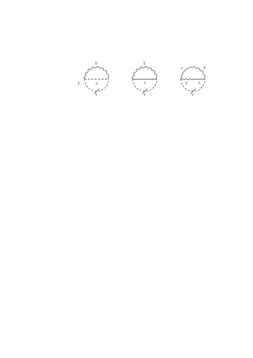
Figure 1: Vacuum diagrams contributing to the leading order equation of $G_{\pi}$ (cf. the “setting sun” integrals of (23) containing $G_{\pi}$ and proportional to $n^{2}$). One pion line is cut corresponding to the variation of the 2PI effective potential with respect to the pion propagator.

The following zeroth order (tree-level) propagator matrices from (7) will also appear in the 2PI effective potential:

$$i{\cal D}_{(s,Y)}^{-1}=\begin{pmatrix}~{}iD_{0}^{-1}~{}&~{}2i\sqrt{g_{2}}v~{}\\ ~{}2i\sqrt{g_{2}}v~{}&~{}-1~{}\end{pmatrix},\qquad\displaystyle i{\cal D}_{(X,Y^{0},s^{0})}^{-1}=\begin{pmatrix}~{}-1~{}&0&~{}2i\sqrt{g_{1}}v~{}\\ 0&-1&~{}2i\sqrt{g_{2}}v~{}\\ ~{}2i\sqrt{g_{1}}v~{}&~{}2i\sqrt{g_{2}}v~{}&iD_{0}^{-1}\\ \end{pmatrix}.$$ (21)

At this point it is convenient to introduce the rescaled variables

$$x=\frac{\sqrt{2g_{1}}}{n}X,\qquad y^{0}=\frac{\sqrt{2g_{2}}}{n}Y^{0},$$ (22)

which leads to $M^{2}=m^{2}-i(x+y^{0})$. Using (11), (16), (19) and (20), one writes

$$V^{2PI} = n^{2}(m^{2}v^{2}-2hv)+\frac{n^{2}}{4}\left(\frac{1}{g_{1}}x^{2}+\frac{1}{g_{2}}(y^{0})^{2}\right)-in^{2}(y^{0}+x)v^{2}$$ (23)

$$-i\frac{n^{2}}{2}\int_{k}(\ln G_{\pi}^{-1}(k)+D_{0}^{-1}(k)G_{\pi}(k))-i\frac{n^{2}}{2}\int_{k}\textrm{Tr}[\ln{\cal G}_{(s,Y)}^{-1}(k)+{\cal D}_{(s,Y)}^{-1}(k){\cal G}_{(s,Y)}(k)]$$

$$-i\frac{1}{2}\int_{k}(\ln G_{\pi^{0}}^{-1}(k)+D_{0}^{-1}(k)G_{\pi^{0}}(k))-i\frac{1}{2}\int_{k}\textrm{Tr}[\ln{\cal G}_{(X,Y^{0},s^{0})}^{-1}(k)+{\cal D}_{(X,Y^{0},s^{0})}^{-1}(k){\cal G}_{(X,Y^{0},s^{0})}(k)]$$

$$+i\frac{n^{2}}{4}g_{2}\int_{k}\int_{p}\Big{[}\Big{(}G_{\pi}(k)G_{\pi}(k+p)+G_{s}(k)G_{s}(k+p)\Big{)}G_{Y}(p)+2G_{sY}(k)G_{sY}(k+p)G_{s}(p)\Big{]}$$

$$+i\frac{n^{2}}{2}g_{2}~{}\int_{k}\int_{p}\Big{(}G_{Y}(k)G_{s}(k+p)-G_{sY}(k)G_{sY}(k+p)\Big{)}G_{\pi}(p)$$

$$+i\frac{1}{2}g_{1}\int_{k}\int_{p}\Big{(}G_{s}(k)G_{s}(k+p)+G_{\pi}(k)G_{\pi}(k+p)\Big{)}G_{X}(p)$$

$$+i\sqrt{g_{1}g_{2}}\int_{k}\int_{p}\Big{(}G_{s}(k)G_{s}(k+p)+G_{\pi}(k)G_{\pi}(k+p)\Big{)}G_{XY^{0}}(p)$$

$$+i\frac{1}{2}g_{2}\int_{k}\int_{p}\Big{(}G_{s}(k)G_{s}(k+p)+G_{\pi}(k)G_{\pi}(k+p)\Big{)}G_{Y^{0}}(p)$$

$$+2i\sqrt{g_{1}g_{2}}\int_{k}\int_{p}G_{sY}(k)G_{s}(k+p)G_{s^{0}X}(p)+2ig_{2}\int_{k}\int_{p}G_{sY}(k)G_{s}(k+p)G_{s^{0}Y^{0}}(p)$$

$$+i\frac{1}{2}g_{2}\int_{k}\int_{p}\Big{(}G_{s}(k)G_{Y}(k+p)+G_{sY}(k)G_{sY}(k+p)\Big{)}G_{s^{0}}(p)$$

$$+ig_{2}\int_{k}\int_{p}G_{Y}(k)G_{\pi}(k+p)G_{\pi^{0}}(p)+V^{2PI}_{ct}.$$

Since the $\pi$ and the $s-Y$ sectors are of multiplicity ($n^{2}-1$), some ${\cal{O}}(1)$ terms in (23) are not relevant for their leading order equations. These contributions were therefore not written out explicitly in (16) and (17). There are ${\cal{O}}(1)$ terms of the complete effective potential, which contribute only to the $\pi$ or $s-Y$ sector (at NLO), these are omitted from (23). However, for the remaining propagators it is necessary to take into account the proper ${\cal{O}}(1)$ terms, which are therefore included in (23). This means, that (23) is not a large-$n$ expanded 2PI effective potential truncated at 2-loop level. Note, that the structure appearing in the fifth line corresponds to a setting-sun diagram with antisymmetrized vertex functions (e.g. $\sim f^{abc}$).

In $V^{2PI}_{ct}$ one collects all counterterms, which should ensure the finiteness of the equations. One can introduce counterterms to all independent pieces appearing in the mean-field part of the effective potential and independently of them also to the terms showing up in the inverse tree-level propagators. Note, that one might have to introduce counterterms also to pieces which are chosen to have a fixed numerical (zero or unity) renormalized coefficient. No counterterms are introduced corresponding to the setting-sun contributions, since these couplings are kept at their classical value. In this sense the most general form which we will need and is allowed by the structure of $V^{2PI}$ is the following:

$$V^{2PI}_{ct} = n^{2}\delta m^{2}_{0}v^{2}+\frac{n^{2}}{4}\Big{(}\delta_{x}x^{2}+\delta_{y}(y^{0})^{2}\Big{)}+\frac{n^{2}}{2\sqrt{g_{1}g_{2}}}\delta_{xy}xy^{0}-in^{2}v^{2}(\delta_{yv}y^{0}+\delta_{xv}x)-in^{2}(\delta_{y0}y^{0}+\delta_{x0}x)$$ (24)

$$-i\int_{k}\left[\frac{n^{2}}{2}\delta_{YY}G_{Y}(k)+\delta_{XX}G_{X}(k)+\delta_{Y^{0}Y^{0}}G_{Y^{0}}(k)+2\delta_{XY^{0}}G_{XY^{0}}(k)\right]$$

$$-\frac{n^{2}}{2}\int_{k}\left[(\delta Z_{\pi}k^{2}-\delta m^{2}_{\pi}+i\delta_{x\pi}x+i\delta_{y\pi}y^{0})G_{\pi}(k)+(\delta Z_{s}k^{2}-\delta m^{2}_{s}+i\delta_{xs}x+i\delta_{ys}y^{0})G_{s}(k)\right]$$

(the self-energy corrections to $G_{sY}^{-1}$ turn out to be finite). In the first line, countercouplings proportional to $xy^{0},y^{0},x$ will be also needed despite the fact that one chooses the corresponding renormalized values to vanish. Similarly, countercouplings in the second line belong to the contribution of the (pure) auxiliary propagators occurring in terms of the type ${\textrm{Tr}}{\cal D}^{-1}{\cal G}$, in which all their renormalized coefficients are fixed to unity except the coefficient of $G_{XY^{0}}$, which is zero. In the third line, countercouplings are introduced to the terms appearing in $D^{-1}_{ss}$ and $D^{-1}_{\pi}$. In the exact solution of the theory only unique quadratic and quartic counterterms should occur, but in any finite order of a 2PI approximation one has the freedom to choose the countercouplings in the counterterm functional independently berges05 . For the determination of (24) one should analyze the divergence structure of the integrals appearing in the propagator equations.

IV A self-consistent assumption on mass hierarchy

The assumption, that the scalar sector is considerably heavier than the pionic simplifies the solution of the limiting form of the coupled Dyson-Schwinger equations valid at infinite $n$. In addition, we assume that the scalar masses are considerably larger than the amplitude of the symmetry breaking vacuum condensate. Each component of the propagators in the mixed sectors will have a common denominator displaying the corresponding heavy mass. Therefore the only consequent way to neglect in a first approximation the heavy sector is to neglect the bubble contributions containing at least one component of ${\cal G}_{(s,Y)}$ or ${\cal G}_{(X,Y^{0},s^{0})}$. Then, in a first approximation only bubble diagrams exclusively built with $G_{\pi}$ are included. This means that in (16) all bubbles are suppressed, while in (19) and (20) only the unique pure pion bubble remains.

IV.1 Retaining only the light pion dynamics

The first consequence is that all $n^{2}$ pion propagators are equal to their tree-level value, and therefore have the same mass: $M^{2}_{\pi^{a}}=M^{2}$. The explicit form of the saddle-point equations can be written with the help of splitting the pion tadpole into finite $(T_{\pi}^{F})$ and divergent parts [for the definitions of $T_{d}^{(2)},T_{d}^{(0)}$ see Appendix A.] as

$$\int_{k}G_{\pi}(k)=T_{\pi}^{F}+T_{d}^{(2)}+(M^{2}-M_{0}^{2})T_{d}^{(0)},$$ (25)

and using the counterterms it becomes the following:

$$\frac{x}{g_{1}}=i\Big{(}2v^{2}+T_{d}^{(2)}+(M^{2}-M_{0}^{2})T_{d}^{(0)}+T_{\pi}^{F}\Big{)}-\Big{(}\delta_{x}x+\delta_{xy}\frac{1}{\sqrt{g_{1}g_{2}}}y^{0}\Big{)}+2i\delta_{x0},$$

$$\frac{y^{0}}{g_{2}}=i\Big{(}2v^{2}+T_{d}^{(2)}+(M^{2}-M_{0}^{2})T_{d}^{(0)}+T_{\pi}^{F}\Big{)}-\Big{(}\delta_{y}y^{0}+\delta_{xy}\frac{1}{\sqrt{g_{1}g_{2}}}x\Big{)}+2i\delta_{y0}.$$ (26)

It turns out, that at this level the other counterterms (e.g. $\delta_{xv},\delta_{x\pi},\delta_{xs},\delta_{yv},\delta_{y\pi},\delta_{ys}$) are zero, therefore for the sake of transparency we did not written them out explicitly in (26). Taking into account the definition (13) of $M^{2}$, the following counterterms renormalize both equations:

$$\delta_{x}=\delta_{y}=T_{d}^{(0)},\qquad\delta_{x0}=\delta_{y0}=-\frac{1}{2}\left(T_{d}^{(2)}+(m^{2}-M_{0}^{2})T_{d}^{(0)}\right),\qquad\delta_{xy}=\sqrt{g_{1}g_{2}}T_{d}^{(0)}.$$ (27)

Because of the omission of the last (”heavy”) term in the third equation of (11), the equation of state does not require any extra counterterm. The finite equations for the 1-point functions read as follows:

$$\frac{x}{g_{1}}=i(2v^{2}+T_{\pi}^{F}),\qquad\frac{y^{0}}{g_{2}}=i(2v^{2}+T_{\pi}^{F}),\qquad M^{2}v=h.$$ (28)

The $2\times 2$ propagator matrix of the $(s,Y)$ sector simplifies to

$$i{\cal G}_{(s,Y)}^{-1}(k)=\begin{pmatrix}~{}iD_{0}^{-1}(k)~{}&~{}2i\sqrt{g_{2}}v~{}\\ ~{}2i\sqrt{g_{2}}v~{}&~{}-1+i\delta_{YY}+\frac{g_{2}}{2}I_{\pi}(k,M)~{}\end{pmatrix},$$ (29)

where we have introduced the function $I_{\pi}(k,M)=-i\int_{p}D_{0}(p)D_{0}(p+k)$ and also written down the contribution obtained from $V^{2PI}_{ct}$. By choosing

$$\delta_{YY}=i\frac{g_{2}}{2}T_{d}^{(0)},$$ (30)

one ensures the finiteness of the matrix elements. The squared scalar mass is determined by the zero of the determinant:

$$M_{(s,Y)}^{2}=M^{2}+4g_{2}v^{2}\frac{1}{1-\frac{g_{2}}{2}I_{\pi}^{F}(k=M_{(s,Y)},M)}.$$ (31)

The mass matrix of the $(X,Y^{0},s^{0})$ sector also becomes more transparent:

$$i{\cal G}_{(X,Y^{0},s^{0})}^{-1}=\begin{pmatrix}~{}-1+2i\delta_{XX}+g_{1}I_{\pi}(k)~{}&~{}2i\delta_{XY^{0}}+\sqrt{g_{1}g_{2}}I_{\pi}(k)~{}&~{}2i\sqrt{g_{1}}v~{}\\ ~{}2i\delta_{XY^{0}}+\sqrt{g_{1}g_{2}}I_{\pi}(k)~{}&~{}-1+2i\delta_{Y^{0}Y^{0}}+g_{2}I_{\pi}(k)~{}&~{}2i\sqrt{g_{2}}v~{}\\ ~{}2i\sqrt{g_{1}}v~{}&~{}2i\sqrt{g_{2}}v~{}&~{}iD_{0}^{-1}(k)~{}\end{pmatrix},$$ (32)

which after introducing the obvious counterterms

$$\delta_{XX}=\frac{i}{2}g_{1}T_{d}^{(0)},\qquad\delta_{XY^{0}}=\frac{i}{2}\sqrt{g_{1}g_{2}}T_{d}^{(0)},\qquad\delta_{Y^{0}Y^{0}}=\frac{i}{2}g_{2}T_{d}^{(0)}$$ (33)

leads to a determinant equation completely analogous to the previous one:

$$M_{(X,Y^{0},s^{0})}^{2}=M^{2}+4(g_{1}+g_{2})v^{2}\frac{1}{1-(g_{1}+g_{2})I^{F}_{\pi}(k=M_{(X,Y^{0},s^{0})},M)}.$$ (34)

One can see, that the spectra resulting from the assumption we made for the mass hierarchy might be consistent with the outcome in the sense that the scalar sector (and the auxiliary fields hybridized with it) can be indeed heavier than the pionic one.

In the next subsection we investigate the region of the parameter space, where the scalar masses become much heavier than the pseudoscalars ensuring the self-consistency of our approximate solution.

IV.2 Validity of the mass assumption

First one has to note, that in the case when no explicit symmetry breaking term is added to the Lagrangian ($h=0$) the mass assumption is true, since our approximation preserves Goldstone’s theorem and therefore makes the pions massless, which means that they are ”infinitely” lighter than the scalars.

The interesting case is when $h\neq 0$. Let us define $r_{s,Y}:=M_{(s,Y)}/M$ and $r_{X,Y^{0},s^{0}}:=M_{(X,Y^{0},s^{0})}/M$. In order to obtain a proper region of the parameter space, we introduce a heaviness criterium: the scalars are heavy enough if relations $r_{s,Y}>r_{0}$, $r_{X,Y^{0},s^{0}}>r_{0}$ hold simultaneously, where $r_{0}$ is a given number. It is somewhat arbitrary what value to choose for $r_{0}$. In this exploratory study, we work with the convenient choice $r_{0}=2$, because the quantity $I_{\pi}^{F}(k,M)$ appearing in both gap equations (31) and (34) develops an imaginary part just for $k^{2}>4M^{2}$ (two-pion threshold). Above the threshold the masses are defined as real parts of the complex solutions. Expressing $v$ from the EoS in (28), the two relevant equations are the following:

$$M_{(s,Y)}^{2} = M^{2}+4g_{2}\frac{h^{2}}{M^{4}}\frac{1-\frac{g_{2}}{2}\Re I_{\pi}^{F}(k=M_{(s,Y)},M)}{[1-\frac{g_{2}}{2}\Re I_{\pi}^{F}(k=M_{(s,Y)},M)]^{2}+[\frac{g_{2}}{2}\Im I_{\pi}^{F}(k=M_{(s,Y)},M)]^{2}},$$ (35)

$$M_{(X,Y^{0},s^{0})}^{2} = M^{2}+4(g_{1}+g_{2})\frac{h^{2}}{M^{4}}\frac{1-(g_{1}+g_{2})\Re I_{\pi}^{F}(k=M_{(X,Y^{0},s^{0})},M)}{[1-(g_{1}+g_{2})\Re I_{\pi}^{F}(k=M_{(X,Y^{0},s^{0})},M)]^{2}+[(g_{1}+g_{2})\Im I_{\pi}^{F}(k=M_{(X,Y^{0},s^{0})},M)]^{2}}.$$

The bubble integrals are given by (A3). It is convenient to express all masses in proportion to the absolute value of the renormalized mass $(\sqrt{|m^{2}|})$, which means practically to write the definition of the pion mass as $M^{2}=-1-ix-iy_{0}$. With the use of (28) and (A4), one gets

$$M^{2}=-1+(g_{1}+g_{2})\Big{(}\frac{2h^{2}}{M^{4}}+\frac{M^{2}}{16\pi^{2}}\log\frac{eM^{2}}{M_{0}^{2}}\Big{)},$$ (36)

where $M_{0}$ is the renormalization scale. For fixed $M_{0}$, in the original units (36) determines $M^{2}/|m^{2}|$ as a function of $h/|m|^{3},g_{1},g_{2}$. Plugging it into the scalar gap equations, they can be solved for $M_{(s,Y)}/\sqrt{|m^{2}|}$ and $M_{(X,Y^{0},s^{0})}/\sqrt{|m^{2}|}$. Then, one can trace out the region, where the heaviness criterium is fulfilled. This region is the part of the positive $g_{1}-g_{2}$ octant (the stability region of the $n\rightarrow\infty$ theory) below the surface displayed in Fig. 2. As expected, the projection of the allowed region onto the $g_{1}-g_{2}$ plane shrinks for increasing value of $h/|m|^{3}$. We have varied $M_{0}/\sqrt{|m|^{2}}$ in the interval $(1,10)$ and only a mild displacement of the allowed region could be observed without really changing the shape. This change can be balanced by an appropriate Renormalization Group transformation of the quartic couplings, e.g. using $g_{i}=g_{i}(M_{0})$.

The modification of the allowed region occuring when the spectra is corrected by the fluctuations of the heavy scalars will be discussed in a forthcoming publication.

Figure 2: Region of the parameter space, where the mass assumption holds (using renormalization scale $M_{0}/\sqrt{|m^{2}|}=2.5$)

IV.3 Heavy scalar corrections

Using the propagators of the coupled $(s,Y)$-sector, one can start to systematically take into account the effect of the heavy degrees of freedom on the pion propagator, the EoS and the SPEs. In particular we now invoke the tadpole and bubble contributions to these equations evaluated with (29). For this we write explicitly the components of the heavy scalar propagator matrix:

$$\displaystyle G_{s}(k)=\frac{i}{d(k)}\left(1-\frac{g_{2}}{2}I_{\pi}^{F}(k)\right),\quad G_{Y}(k)=-\frac{i}{d(k)}(k^{2}-M^{2}),\quad G_{sY}(k)=-\frac{1}{d(k)}2\sqrt{g_{2}}v,$$

$$\displaystyle d(k)=\left(1-\frac{g_{2}}{2}I_{\pi}^{F}(k)\right)(k^{2}-M^{2})-4g_{2}v^{2}.$$ (37)

With the help of these expressions, one readily writes the scalar tadpole contributions to the SPEs. The correction of the EoS is of imminent interest, since it has an important role in the discussion of the validity of Goldstone’s theorem. Using the expression of $G_{sY}$, one finds the unrenormalized equation of state:

$$M^{2}+2g_{2}\int_{p}\frac{i}{d(p)}=\frac{h}{v}.$$ (38)

Now we proceed with the unrenormalized pion propagators:

$$iG_{\pi^{0}}^{-1}(k) = k^{2}-M^{2}-2g_{2}\int_{p}\frac{i}{d(p)}\frac{p^{2}-M^{2}}{(k-p)^{2}-M^{2}},$$

$$iG_{\pi}^{-1}(k) = k^{2}-M^{2}-g_{2}\int_{p}\frac{i}{d(p)}\frac{p^{2}-M^{2}}{(k-p)^{2}-M^{2}}$$ (39)

$$+4g_{2}^{2}v^{2}\int_{p}\frac{i}{d(p)d(k-p)}-ig_{2}\int_{p}\frac{(p^{2}-M^{2})(1-g_{2}I_{\pi}^{F}(k-p)/2)}{d(p)d(k-p)}.$$

When one sets $k=0$, both propagator equations turn out to be the same. Comparing to the equation of state one finds, that the approximation fulfills the Goldstone theorem characterizing the $U(n)\times U(n)\rightarrow U(n)$ symmetry breaking. It will be demonstrated in the next section, that both equations receive the same counterterm contributions.

Since the tadpoles of $G_{s}$ and $G_{sY}$ play a role in the EoS and the SPEs, it is worthwhile to investigate their corrections, although these contributions should be considered only as NNLO “heavy” corrections. Substituting the leading order propagators into the second term on the right hand side of the equation of $G_{sY}^{-1}$ (17), one finds for the $\Sigma_{sY}$ self-energy:

$$\Sigma_{sY}(p)\equiv ig_{2}\int_{k}G_{sY}(p-k)\Big{(}G_{s}(k)-G_{\pi}(k)\Big{)}=-8g_{2}^{2}\sqrt{g_{2}}v^{3}\int_{k}\frac{1}{d(p-k)d(k)(k^{2}-M^{2})},$$ (40)

which does not induce any counterterm, since it is finite. The heavy correction to $G_{s}^{-1}$ is very similar to that of $G^{-1}_{\pi}$ in (39):

$$iG_{s}^{-1}(k) = k^{2}-M^{2}-g_{2}\int_{p}\frac{i}{d(p)}\frac{p^{2}-M^{2}}{(k-p)^{2}-M^{2}}$$ (41)

$$-4g_{2}^{2}v^{2}\int_{p}\frac{i}{d(p)d(k-p)}-ig_{2}\int_{p}\frac{(p^{2}-M^{2})(1-g_{2}I_{\pi}^{F}(k-p)/2)}{d(p)d(k-p)}.$$

The scalar corrections are taken into account also in the SPEs. They appear partly directly via the scalar tadpole, and also by the scalar correction of the pion tadpole. The structure of the two SPE’s in (11) is identical in view of (12), therefore it is sufficient to investigate the equation, which determines $x$. The unrenormalized form of the saddle-point equation reads as follows:

$$0=\frac{x}{g_{1}}-2iv^{2}-i\int_{k}\left(G_{s}(k)+G_{\pi}(k)\right).$$ (42)

The expression of the scalar tadpole is readily written down. The pion tadpole is expanded to linear order in the $\Sigma_{\pi}$ self-energy contribution:

$$-i\int_{k}G_{\pi}(k)\approx-i\int_{k}D_{0}(k)+\int_{k}\frac{1}{(k^{2}-M^{2})^{2}}\Sigma_{\pi},$$ (43)

where

$$\Sigma_{\pi}(k)=g_{2}\int_{p}\frac{i}{d(p)}\left[\frac{p^{2}-M^{2}}{(k-p)^{2}-M^{2}}-\frac{4g_{2}v^{2}}{d(k-p)}+\frac{(p^{2}-M^{2})(1-g_{2}I^{F}_{\pi}(k-p)/2)}{d(k-p)}\right].$$ (44)

All these equations need (resummed) renormalization, which is discussed in detail in the next section. Note, that in this process the counterterms (27), which were determined on the level of pure pionic fluctuations receive further contributions. Also, the yet unused counterterms (except $\delta Z_{s},\delta Z_{\pi}$ counterterms proportional to wave function renormalization) will get nonzero values.

V Divergence analysis and renormalizability

The separation of the divergences in the EoS, the corrections to the pion propagator and the SPEs rely very heavily on our previous analysis of the NLO renormalization of the $O(N)$ model fejos09 . Most of the divergent integrals occurring in the present analysis can be made finite with the subtraction of the appropriate combinations of divergent integrals defined there. For the reader’s convenience we list those, which are used here in Appendix A.

Let us start the divergence analysis with the EoS. The integral appearing in it can be expanded for large momenta in powers of $4g_{2}v^{2}$:

$$\int_{p}\frac{i}{d(p)}=\int_{p}\frac{i}{(p^{2}-M^{2})(1-g_{2}I_{\pi}^{F}(p)/2)}\left(1+\frac{4g_{2}v^{2}}{(p^{2}-M^{2})(1-g_{2}I_{\pi}^{F}(p)/2)}+...\right).$$ (45)

Only the first term of this expansion is divergent and its divergence is given in (A5) with $\gamma=g_{2}/2$:

$$\int_{p}\frac{i}{d(p)}\Big{|}_{div}=T_{a}^{(2)}-\frac{3g_{2}}{2}(M^{2}-M_{0}^{2})T_{a}^{(I)}.$$ (46)

From here one finds for the corresponding countercouplings of (24):

$$\delta m_{0}^{2}=-2g_{2}\left(T_{a}^{(2)}-\frac{3g_{2}}{2}(m^{2}-M_{0}^{2})T_{a}^{(I)}\right),\qquad\delta_{xv}=\delta_{yv}=3g_{2}^{2}T_{a}^{(I)}.$$ (47)

Next we proceed with the $\Sigma_{\pi}$ self-energy. The second of the three bubble integrals appearing in the expression of the heavy scalar corrections to $G^{-1}_{\pi}$ (39) is finite. The first integral can be written in power series with respect to $4g_{2}v^{2}$ as

$$-ig_{2}\int_{p}\frac{1}{d(p)}\frac{p^{2}-M^{2}}{(k-p)^{2}-M^{2}}$$

$$=-ig_{2}\int_{p}\frac{1}{(p^{2}-M^{2})(1-g_{2}I_{\pi}^{F}(p)/2)}\left(1+\frac{4g_{2}v^{2}}{(p^{2}-M^{2})(1-g_{2}I_{\pi}^{F}(p)/2)}+...\right)\frac{p^{2}-M^{2}}{(k-p)^{2}-M^{2}}.$$ (48)

One recognizes again, that only the integral of the first term of the expansion is divergent. This is exactly the integral which was shown in Eq. (A7) of fejos09 to not have momentum dependent divergence. The same analysis leads also in case of the third integral to the same divergent piece. Therefore one concludes $\delta Z_{\pi}=0$.

In view of this, one can put $k=0$ in the pion propagator and find its divergences. Since Goldstone’s theorem is obeyed, the same divergences occur as in the EoS. As a consequence one has in (24)

$$\delta m_{\pi}^{2}=\delta m_{0}^{2},\qquad\delta_{x\pi}=\delta_{xv},\quad\delta_{y\pi}=\delta_{yv}.$$ (49)

Using these results, one can find promptly the counterterms proportional to the $G_{s}$ tadpole in (24). Since the divergent pieces of $\Sigma_{s}$ coincide with those appearing in $\Sigma_{\pi}$, one has

$$\delta Z_{s}=0,\qquad\delta m_{s}^{2}=\delta m_{0}^{2},\qquad\delta_{xs}=\delta_{xv},\qquad\delta_{ys}=\delta_{yv}.$$ (50)

These equalities reflect the fact, that the ultraviolet behavior of the $\pi$ and $s$ multiplets are the same, irrespective of the symmetry breaking pattern and the structure of the mass spectrum.

At this stage we have specified the expressions of the countercouplings of the counterterm functional (24), up to the scalar corrections of the purely $X,Y^{0}$-dependent divergences. The renormalized SPE of $x$ takes a very transparent form, when the results of the above analysis are taken into account:

$$0=\frac{x}{g_{1}}-2i\left(v^{2}+\frac{1}{2}\int_{k}(G_{s}(k)+G_{\pi}(k))\right)(1+\delta_{xv})+\delta_{x}x-2i\delta_{x0}+\frac{1}{\sqrt{g_{1}g_{2}}}\delta_{xy}y^{0}.$$ (51)

The last three terms represent the counterterms, which cancel those divergences of the tadpole integrals, which depend solely on $x$ and $y^{0}$. The consistency with the previous steps of the renormalization requires the cancellation of the “dangerous” product $\delta_{xv}(2v^{2}+\int G_{s}|_{F}+\int G_{\pi}|_{F})\equiv\delta_{xv}(2v^{2}+T_{s}^{F}+T_{\pi}^{F})$ without the need for any new counterterm (which would react back on the EoS and the equation of the pion’s 2-point function). The unique common divergent coefficient in front of this sum is expected to prevail in the exact renormalized equation, since it is the result of the Goldstone theorem and of the $U(n)\times U(n)$ symmetry valid in the ultraviolet regime.

The contributions cancelling the above counterterm contribution come from the heavy corrections to the pion tadpole and from the scalar tadpole eventually also modified by the heavy corrections. This cancellation can not be complete on the level of the first round of heavy corrections, since then the scalar tadpole does not give any divergent term proportional to $T_{s}^{F}$ which would be able to cancel $\delta_{xv}T_{s}^{F}$. However, this latter should be invoked first in the second iteration of the heavy corrections, therefore one simply omits it at this stage of the iteration, and no imbalance is detected in the divergences proportional to $T_{s}^{F}$.

The actual form of the SPE (51) is the following after the first round of the heavy corrections:

$$0=\frac{x}{g_{1}}-2i\left(v^{2}+\frac{1}{2}\int_{k}(G_{s}(k)+G_{\pi}(k))\right)-2i\left(v^{2}+\frac{1}{2}\int_{k}D_{0}(k)\right)\delta_{xv}+\delta_{x}x-2i\delta_{x0}+\frac{1}{\sqrt{g_{1}g_{2}}}\delta_{xy}y^{0}.$$ (52)

Here one has to consider the pion tadpole as the sum displayed in (43). The contribution of the scalar tadpole when expanded in powers of $4g_{2}v^{2}$ can be written as follows:

$$-i\int_{k}G_{s}(k)=-i\int_{k}\frac{i}{k^{2}-M^{2}}\left(1+4g_{2}v^{2}\frac{1}{(k^{2}-M^{2})(1-g_{2}I^{F}_{\pi}(k)/2)}+...\right)$$ (53)

Only these two terms, written out explicitly, contain divergences, therefore

$$-i\int_{k}G_{s}(k)\Big{|}_{div} = -i[T_{d}^{(2)}+(M^{2}-M_{0}^{2})T_{d}^{(0)}]-4ig_{2}v^{2}\int_{k}\frac{i}{(k^{2}-M^{2})^{2}(1-g_{2}I^{F}_{\pi}(k)/2)}\Big{|}_{div}$$ (54)

$$= -i[T_{d}^{(2)}+(M^{2}-M_{0}^{2})T_{d}^{(0)}]+2ig_{2}^{2}v^{2}T_{a}^{(I)}.$$

Every term, except the last one on the right-hand side can be cancelled by appropriate extensions of the counterterms at most quadratic in $x$ and $y^{0}$ [see (27)]. The heavy correction of the pion tadpole has the following expression:

$$\Delta\left[-i\int_{k}G_{\pi}(k)\right] = -ig_{2}\int_{k}\frac{i}{(k^{2}-M^{2})^{2}}\times$$ (55)

$$\left(\int_{p}\frac{i}{d(p)}\left(\frac{p^{2}-M^{2}}{(k-p)^{2}-M^{2}}-\frac{4g_{2}v^{2}}{d(k-p)}+\frac{(p^{2}-M^{2})(1-g_{2}I^{F}_{\pi}(k-p)/2)}{d(k-p)}\right)\right)_{finite}.$$

The part of the divergence which is independent of $v^{2}$ is separated as

$$\Delta\left[-i\int_{k}G_{\pi}(k)\right]\Bigg{|}_{v=0,div}=2ig_{2}\left[\int_{k}\frac{1}{(k^{2}-M^{2})^{2}}\left(\int_{p}\frac{1}{((k-p)^{2}-M^{2})(1-g_{2}I_{\pi}^{F}(p,M)/2)}\right)_{finite}\right]_{div}$$ (56)

Using (A12) of Appendix A., one finds

$$\Delta\left[-i\int_{k}G_{\pi}(k)\right]\Bigg{|}_{v=0,~{}div}=-2ig_{2}(A_{div}+B_{div}M^{2})+3ig_{2}^{2}T_{\pi}^{F}(M)T_{a}^{(I)}.$$ (57)

The last term when substituted into (52) exactly compensates the dangerous term $-i\delta_{xv}T^{F}_{\pi}(M)$, which arises from the $-i\delta_{xv}\int D_{0}$ term. The appearing new divergences (proportional to $A_{div}$ and $B_{div}$) can be compensated by adding further heavy corrections to (27). The consistent cancellation of the divergences proportional to $T_{\pi}^{F}$ could have been anticipated, since the counterterm proportional to the scalar tadpole left out from (51) at this level cannot lead to any divergence proportional to $T_{\pi}^{F}$. Therefore in this respect (52) does not differ from the exact relation (51).

Next, one turns to the prospectively divergent terms proportional to $v^{2}$ of the SPE contributed by the pion tadpole:

$$-4ig_{2}^{2}v^{2}\int_{k} \frac{i}{(k^{2}-M^{2})^{2}}\times$$ (58)

$$\Bigl{[}2\int_{p}\frac{i}{(p^{2}-M^{2})((k-p)^{2}-M^{2})(1-g_{2}I^{F}_{\pi}(p)/2)^{2}}$$

$$+\int_{p}\frac{i}{((k-p)^{2}-M^{2})(1-g_{2}I_{\pi}^{F}(k-p)/2)(1-g_{2}I^{F}_{\pi}(p)/2)}\left(\frac{1}{(k-p)^{2}-M^{2}}-\frac{1}{p^{2}-M^{2}}\right)\Bigr{]}.$$

One finds by inspection, that there is no subdivergence in this expression. The first term of the square bracket produces an overall divergent piece $8ig_{2}^{2}v^{2}T_{a}^{(I)}$. It can be found following the previous line of analysis, e.g. after changing the order of integration performing the $k$-integration first. A careful, but rather lengthy analysis leads to the conclusion, that the second double integral is finite.

Eventually one finds that in the sum the three divergent contributions proportional to $v^{2}$ do not annihilate. It is easy to see, at least partially, the source of this imbalance. When in a subsequent iteration round one uses in the scalar tadpole a propagator involving heavy corrections, it also produces a divergent contribution proportional to $ig_{2}^{2}v^{2}T_{a}^{(I)}$. This shows that in case of this single type of divergence for the cancellation one has to take into account contributions belonging to different iteration levels of the heavy contributions. Actually, all this is not unexpected, since the ultraviolet features of the integrals are independent of any hierarchy in the spectra. Therefore in practice, one renormalizes the saddle-point equations subtracting the remainder of the divergences proportional to $v^{2}$ by hand.

VI Conclusions and outlook

A leading large-$n$ solution was presented in a ground state, which breaks the $U(n)\times U(n)$ symmetry of the Lagrangian to $U(n)$. In the construction of the solution, a light pseudoscalar/heavy scalar hierarchy of the spectra was assumed. The renormalizability of the equation of state and propagator equations, is a precondition for the investigation of the consistency of this additional assumption. This feature was demonstrated by constructing the counterterms to the equations above. The consistency of these counterterms required an additional subtraction for the renormalization of the saddle-point equations. It was shown, that the proposed solution explicitly fulfills Goldstone’s theorem. The pions are generically light, therefore the assumed mass hierarchy will not be erased by heavy radiative corrections, as was demonstrated by our exploratory investigation. It is probably present in a large part of the $(g_{1},g_{2})$ coupling-plane.

The proposed procedure of constructing a leading large-$n$ solution for the $U(n)\times U(n)\rightarrow U(n)$ symmetry breaking pattern can be developed further in several directions. In the range of validity of the mass hierarchy we shall study the finite temperature features of the proposed solution. The relevance of it would be largely strengthened, if a first order symmetry restoring transition were found in agreement with the renormalization group argument. For the applications to strong interaction phenomena at $n=3$ one ought to introduce also the $U_{A}(1)$ breaking effective (determinant) term as a sort of perturbation to this solution. A simple realization could be to include its contribution into the two-loop 2PI effective potential of the model and evaluate it with approximate large-$n$ propagators constructed in this paper. Finally, we note, that one can make use of these propagators also in models, where constituent quarks are coupled to the mesons.

Appendix A Divergences of some relevant integrals

The divergences of the integrals listed below all can be read in somewhat scattered way in fejos09 . Here we summarize them for the reader’s convenience. The divergences are expressed in terms of the following divergent integrals:

$$\displaystyle T_{d}^{(2)}\equiv\int_{k}\frac{i}{k^{2}-M_{0}^{2}},\qquad T_{d}^{(0)}\equiv\int_{k}\frac{i}{(k^{2}-M^{2}_{0})^{2}}$$

$$\displaystyle T_{a}^{(2)}\equiv\int_{k}\frac{i}{(k^{2}-M_{0}^{2})(1-\gamma I_{0}^{F}(k))},\qquad T_{a}^{(I)}\equiv\int_{k}\frac{i}{(k^{2}-M_{0}^{2})^{2}(1-\gamma I_{0}^{F}(k))^{2}}I_{0}^{F}(k),$$ (A1)

where $M_{0}$ is an arbitrary normalization scale which makes these integrals infrared safe, $\gamma$ is a parameter which in case of our model equals $g_{2}/2$, and $I^{F}(k,M)$ is the finite part of the bubble integral

$$I^{F}(k,M)=\int_{p}\frac{i}{(p^{2}-M^{2})((k-p)^{2}-M^{2})}-T_{d}^{(0)}.$$ (A2)

or in more explicit terms with real and imaginary parts separated:

$$\Re I^{F}(k,M) = \frac{1}{16\pi^{2}}\log\frac{M^{2}}{M_{0}^{2}}-\frac{1}{16\pi^{2}}\begin{cases}\sqrt{1-\frac{4M^{2}}{k^{2}}}\log\frac{1-\sqrt{1-\frac{4M^{2}}{k^{2}}}}{1+\sqrt{1-\frac{4M^{2}}{k^{2}}}},\qquad\qquad\qquad k^{2}\geq 4M^{2}\\ -2\sqrt{\frac{4M^{2}}{k^{2}}-1}\arctan[1/\sqrt{1-\frac{4M^{2}}{k^{2}}}],\qquad 4M^{2}>k^{2}>0\\ \sqrt{1-\frac{4M^{2}}{k^{2}}}\log\frac{\sqrt{1-\frac{4M^{2}}{k^{2}}}-1}{\sqrt{1-\frac{4M^{2}}{k^{2}}}+1},\qquad\qquad\qquad 0\geq k^{2}\\ \end{cases}$$

$$\Im I^{F}(k,M) = -\frac{1}{16\pi}\sqrt{1-\frac{4M^{2}}{k^{2}}}\cdot\Theta(k^{2}-4M^{2}).$$ (A3)

The finite part of the tadpole integral is

$$T^{F}(M)=\int_{k}\frac{i}{k^{2}-M^{2}}-(M^{2}-M_{0}^{2})T_{d}^{(0)}-T_{d}^{(2)}\equiv\frac{M^{2}}{16\pi^{2}}\log\frac{M^{2}}{M_{0}^{2}}-\frac{M^{2}-M_{0}^{2}}{16\pi^{2}}$$ (A4)

The divergences of the integrals below were found by replacing the mass parameter $M$ sequentially (with help of subtractions and additions) by the normalization scale $M_{0}$:

$$I_{1}=\int_{k}\frac{i}{(k^{2}-M^{2})(1-\gamma I^{F}(k,M))}\Big{|}_{div}=T_{a}^{(2)}-3\gamma(M^{2}-M_{0}^{2})T_{a}^{(I)}\equiv\tilde{T}_{div}(M^{2}),$$ (A5)

where $I^{F}(k,M)$ is the bubble integral defined with mass $M$. We need in our analysis also the slightly modified integral:

$$I_{1a}=\int_{k}\frac{i}{(k^{2}-4M^{2})(1-\gamma I^{F}(k,M))}\Big{|}_{div}=\tilde{T}_{div}(M^{2})-3\gamma M^{2}T_{a}^{(I)}.$$ (A6)

There is a logarithmically divergent integral:

$$I_{2}=\int_{k}\frac{i}{(k^{2}-M^{2})^{2}(1-\gamma I^{F}(k,M))}\Big{|}_{div}=-\gamma T_{a}^{(I)}.$$ (A7)

The most challenging is the separation of the setting-sun integral, where one subdivergence is already explicitly found:

$$I_{3}=\left[-\int_{k}\frac{i}{(k^{2}-M^{2})^{2}}\left(\int_{p}\frac{1}{((k-p)^{2}-M^{2})(1-\gamma I^{F}(p,M))}\right)_{finite}\right]_{div}.$$ (A8)

Using $I_{1}$ introduced above one can write

$$I_{3}=\left[-\int_{k}\frac{i}{(k^{2}-M^{2})^{2}}\left(\int_{p}\frac{1}{((k-p)^{2}-M^{2})(1-\gamma I^{F}(p,M))}+i\tilde{T}_{div}(M^{2})\right)\right]_{div}.$$ (A9)

After changing the order of the integrals, using (A19) of fejos09 , one is led gradually to the final form of its divergences

$$I_{3} = -\frac{1}{\gamma}\int_{k}\frac{1}{k^{2}-4M^{2}}\Big{|}_{div}+\left(\frac{1}{\gamma}-I^{F}(0,M)+\frac{1}{8\pi^{2}}\right)\int_{k}\frac{1}{(k^{2}-4M^{2})(1-\gamma I^{F}(k,M))}\Big{|}_{div}$$ (A10)

$$-i\tilde{T}_{div}(M^{2})\int_{k}\frac{i}{(k^{2}-M^{2})^{2}}$$

$$= \frac{i}{\gamma}\left[T_{d}^{(2)}+(4M^{2}-M^{2}_{0})T_{d}^{(0)}\right]-i\left[\frac{1}{\gamma}-I^{F}(0,M)+\frac{1}{8\pi^{2}}\right]\left(\tilde{T}_{div}-3\gamma M^{2}T_{a}^{(I)}\right)$$

$$-i\tilde{T}_{div}(M^{2})\left(T_{d}^{(0)}+I^{F}(0,M)\right).$$

The terms proportional to $I^{F}(0,M)$ can be rewritten with the help of a relation between the finite part of the tadpole integral $T^{F}(M)$ and the bubble integral at zero external momentum:

$$M^{2}I^{F}(0,M)=T^{F}(M)+\frac{1}{16\pi^{2}}(M^{2}-M^{2}_{0}).$$ (A11)

In this way one finds a piece linear in $M^{2}$ with somewhat complicated looking divergent coefficients and a dangerous term resulting from an uncancelled subdivergence:

$$I_{3}=i(A_{div}+B_{div}M^{2}-3\gamma T^{F}(M)T_{a}^{(I)}),$$ (A12)

where

$$A_{div}=\frac{1}{\gamma}\Big{[}T_{d}^{(2)}-M_{0}^{2}T_{d}^{(0)}-\tilde{T}_{div}\Big{]}+\frac{3}{16\pi^{2}}\gamma T_{a}^{(I)}M_{0}^{2}-\Big{[}\frac{1}{8\pi^{2}}+T_{d}^{(0)}\Big{]}\tilde{T}_{div},\\$$

$$B_{div}=\frac{4}{\gamma}T_{d}^{(0)}+\Big{[}3+\frac{3\gamma}{16\pi^{2}}\Big{]}T_{a}^{(I)}.$$ (A13)

Appendix B Useful relations involving the $U(n)$ structure constants

In the following relations, the summation over index $e$ (where it appears) goes from $0$ to $n^{2}-1$.

$$\\ f_{0ab}=0,\qquad d_{0ab}=\sqrt{\frac{2}{n}}\delta_{ab},\qquad\sum_{i=1}^{n^{2}-1}d_{0ii}=(n^{2}-1)\sqrt{\frac{2}{n}},\qquad\sum_{i=1}^{n^{2}-1}d_{iia}=\delta_{0a}(n^{2}-1)\sqrt{\frac{2}{n}},$$

$$\sum_{i=1,j\neq 0}^{n^{2}-1}d_{iij}=0,\qquad\sum_{a=0}^{n^{2}-1}d_{aaf}=\sqrt{2n^{3}}\delta_{f0},\qquad\sum_{a=0}^{n^{2}-1}d_{aae}d_{ecd}=2n\delta_{cd},\qquad\sum_{i=1}^{n^{2}-1}d_{iie}d_{ecd}=\frac{2}{n}(n^{2}-1)\delta_{cd},\\$$

$$\sum_{i,j=1}^{n^{2}-1}d_{ijc}d_{ijd}=n\Big{[}1+\delta_{c0}\delta_{d0}-\frac{2}{n^{2}}(2-\delta_{c0}\delta_{d0})\Big{]}\delta_{cd},\qquad\sum_{i=1,a=0}^{n^{2}-1}d_{aic}d_{aid}=n\Big{[}1-\frac{2}{n^{2}}+\delta_{c0}\delta_{d0}\Big{]}\delta_{cd},\\$$

$$\sum_{a=0}^{n^{2}-1}d_{ace}d_{ade}=n(1+\delta_{c0}\delta_{d0})\delta_{cd},\qquad\sum_{i=1}^{n^{2}-1}f_{ice}f_{ide}=n(1-\delta_{c0}\delta_{d0})\delta_{cd}.$$ (B1)

References

- (1) R.D. Pisarski and F. Wilczek, Phys. Rev. D29 (1984) 338
- (2) J.T. Lenaghan, D.H. Rischke and J. Schaffner-Bielich, Phys. Rev. D62 (2000) 085008
- (3) D. Roder, J. Ruppert and D.H. Rischke, Phys. Rev. D68 (2003) 016003
- (4) T. Herpay, A. Patkós, Zs. Szép and P. Szépfalusy, Phys. Rev. D71 (2005) 125017
- (5) P. Kovács and Zs. Szép, Phys. Rev. D77 (2008) 065016
- (6) B.-J. Schaefer and M. Wagner, Phys. Rev. D79 (2009) 014018
- (7) N. Bilic and H. Nikolic, Eur. Phys. J. C6 (1999) 513
- (8) B.-J. Schaefer, M. Wagner and J. Wambach, Phys. Rev. D81 (2010) 074013
- (9) T. Kähära and K. Tuominen, Phys. Rev. D78 (2008) 034015
- (10) H. Mao, J. Jin and M. Huang, J. Phys. G37 (2010) 035001
- (11) U.S. Gupta and V.K. Tiwari, Phys. Rev. D81 (2010) 054019
- (12) G. Markó and Zs. Szép, arXiv:1006.0212
- (13) T. Herbst, J. Pawlowski and B.-J. Schaefer, arXiv:1008.0081
- (14) A. Patkós, Zs. Szép and P. Szépfalusy, Phys. Lett. B537 (2002) 77
- (15) A. Jakovác, A. Patkós, Zs. Szép and P. Szépfalusy, Phys. Lett B582 (2004)
- (16) J. Zinn-Justin, Quantum Field Theory and Critical Phenomena (Clarendon Press, Oxford, 2002) 4th Ed.
- (17) J.O. Andersen, D. Boer and H.J. Warringa, Phys. Rev. D70 (2004) 116007
- (18) J.O. Andersen and T. Brauner, Phys. Rev. D78 (2008) 014030
- (19) G. Fejős, A. Patkós and Zs. Szép, Phys. Rev. D80 025015 (2009)
- (20) T. Appelquist, M. Schwetz and S.B. Selipsky, Phys. Rev. D52 (1995) 4741
- (21) Y. Kikukawa, M. Kohda and J. Yasuda, Phys. Rev. D77 (2008) 015014
- (22) A. J. Paterson, Nucl. Phys. B190 [FS3], 188 (1981)
- (23) R.J. Rivers, Path integral methods in quantum field theory (Cambridge University Press, 1987)
- (24) J. Berges, Introduction to non-equilibrium field theory, AIP Conf. Proc. 739 3 (2004)
- (25) J. Berges, S. Borsanyi, U. Reinosa, J. Serreau, Annals Phys. 320 344 (2005)