Optical tweezers: wideband microrheology

Abstract

Microrheology is a branch of rheology having the same principles as conventional bulk rheology, but working on micron length scales and $\mu l$ volumes.

Optical tweezers have been successfully used with Newtonian fluids for rheological purposes such as determining fluid viscosity. Conversely, when optical tweezers are used to measure the viscoelastic properties of complex fluids the results are either limited to the material’s high-frequency response, discarding important information related to the low-frequency behaviour, or they are supplemented by low-frequency measurements performed with different techniques, often without presenting an overlapping region of clear agreement between the sets of results. We present a simple experimental procedure to perform microrheological measurements over the widest frequency range possible with optical tweezers. A generalised Langevin equation is used to relate the frequency-dependent moduli of the complex fluid to the time-dependent trajectory of a probe particle as it flips between two optical traps that alternately switch on and off.

1 Introduction

Optical tweezers have become an increasingly important tool for the manipulation of micron-scale objects. Taking advantage of the optical gradient force [1] they have been used both as a force sensor [2, 3] and as an force actuator [4, 5]. Though the single beam gradient trap has been around since Ashkin [6], modern holographic optical tweezers, which use spatial light modulators to create multiple optical traps, are capable of moving multiple micron-sized objects in three dimensions [7]. Recent advances in SLM technology mean that optical tweezers are now capable of updating trap positions at hundreds of frames per second with low latency ($\approx$5ms) [8]. This can only serve to broaden the already extensive range of applications for which optical tweezers have been used, such as cell biology [9], investigations into DNA [5], and driving micro-machines [10].

Along with biological and physical experiments optical tweezers have also proved useful for microrheological experiments [11]. Microrheology is concerned with the linear viscoelastic response of materials at microscopic length scales. Such information is invaluable for the investigation of unknown biological processes as well as for increased understanding of the basic physics of fluids. The linear viscoelastic properties of a fluid can be represented by the frequency-dependent dynamic bulk modulus $G^{*}(\omega)$. The dynamic bulk modulus encompasses information about both the elastic and viscous properties of the fluid. It is expressed in the form $G^{*}(\omega)=G^{\prime}(\omega)+iG^{\prime\prime}(\omega)$ [12], where $G^{\prime}(\omega)$ is the frequency-dependent elastic modulus and $G^{\prime\prime}(\omega)$ is the frequency-dependent viscous modulus [13].

As is well known [14, 15, 16], the viscosity of the medium in which a trapped particle is immersed is a key factor affecting the statistical distribution of the particle’s time-dependent position. Hence the viscosity is easily determined from measurements of that distribution. Furthermore, surface effects such as Faxén’s correction to the viscosity of a fluid close to an infinite surface ([15, 16, 17]) have also been widely studied in Newtonian fluids. However when microrheological measurements of viscoelastic substances have been made, results are either limited the high end of the frequency response [18, 19, 20] (omitting the low frequencies entirely) or account is taken of the low frequency response only by the use of complementary techniques such as rotational rheometry [21] or passive video particle tracking microrheology [22]. In both cases this has been done without showing an overlapping region, thus leaving a significant information gap.

The aim of this paper is to present a self-consistent procedure for measuring the linear viscoelastic properties of materials across the widest frequency range achievable with optical tweezers. In particular, the procedure consists of two steps: (I) measuring the thermal fluctuations of a trapped bead for a sufficiently long time; (II) measuring the transient displacement of a bead flipping between two optical traps (spaced at fixed distance $D_{0}$) that alternately switch on/off at sufficiently low frequency. The analysis of the first step (I) provides: (a) the traps stiffness ($\kappa_{i}$, $i=1,2$) — note that this has the added advantage of making the method self-calibrated — and (b) the high frequency viscoelastic properties of the material, to high accuracy. The second step (II) has the potential to provide information about the material’s viscoelastic properties over a very wide frequency range, which is only limited (at the top end) by the acquisition rate of the bead position ($\sim$kH) and (at the bottom end) by the duration of the experiment. However, because of the finite time required by the equipment to switch on/off (i.e. tens of milliseconds), the material’s high-frequency response can not be fully determined by this step. The full viscoelastic spectrum is thus resolved by combining the results obtained from steps (I) and (II).

2 Analytical model

To understand the basis of the procedure, we consider the time-dependent position $\vec{r}(t)$ of a bead trapped by a stationary harmonic potential of force-constant $\kappa_{i}$. Throughout the first step (I) of the procedure, the bead is always found close to the centre of the single trap which is switched on; it makes only small deviations $\vec{r}(t)$ (of magnitude set by the thermal energy) away from the centre of the trap. During step (II) of the procedure, the detours are considerably larger, of a magnitude set by the separation $D_{0}$ of the traps. Let us define $t_{\rm II}$ to be the time at which step (II) commences, i.e. the time at which the traps are first switched. Subsequently, each trap remains on for a duration $P$ before it is switched off and the other trap switched on. Hence the total period of the repeated sequence is $2P$. At the instant immediately after the traps are switched (i.e. at $t=t_{\rm II}+nP$ where $n=0,1\ldots N$), the bead is typically positioned at a distance $\left|\vec{r}(t)\right|\approx D_{0}$ from the centre of the currently active trap (i.e. close to the centre of the trap that has just switched off). Note that coordinates are re-defined so that the bead’s displacement $\vec{r}(t)$ is always measured with respect to the centre of whichever trap is currently switched on. The bead’s position in three dimensions can be modelled by a generalized Langevin equation,

$$m\vec{a}(t)=\vec{f}_{R}(t)-\int^{t}_{t_{0}}\zeta(t-\tau){\vec{v}}(\tau)d\tau-\kappa_{i}\vec{r}(t),$$ (1)

where $m$ is the mass of the particle, $\vec{a}(t)$ is its acceleration, $\vec{v}(t)$ its velocity and $\vec{f}_{R}(t)$ is the usual Gaussian white noise term, modelling stochastic thermal forces acting on the particle. The integral, which incorporates a generalized time-dependent memory function $\zeta(t)$, represents viscoelastic drag from the fluid.

Note that the present method does not require the two traps to be equal. They can be independently, but not simultaneously, calibrated during step I by appealing to the Principle of Equipartition of Energy,

$$\frac{3}{2}k_{B}T=\frac{1}{2}\kappa_{i}\langle r^{2}\rangle,$$ (2)

where $k_{B}$ is Boltzmann’s constant, $T$ is absolute temperature and $\langle r^{2}\rangle$ is the time-independent variance of the particle’s displacement from the trap’s centre. Despite the variety of established methods for determining the stiffness of an optical trap (e.g. using the power spectrum or the drag force [16, 14]), the Equipartition method is the only one independent of the viscoelastic properties of the material under investigation and is thus essential to the calibration of a rheological measurement.

We now examine how Eq. (1) evolves in the two steps (I) and (II). During step (I), the thermal fluctuations of the trapped bead are investigated to determine the high-frequency viscoelastic properties of the material through analysis of the time dependence of the normalised position autocorrelation function $A(\tau)$ (“NPAF”):

$$A(\tau)=\frac{\left\langle\vec{r}(t_{0})\vec{r}(t_{0}+\tau)\right\rangle_{t_{0}}}{\left\langle r(t_{0})^{2}\right\rangle_{t_{0}}},$$ (3)

which, by time-translation invariance, is a function only of the time interval $\tau$. Here, $\left\langle r(t_{0})^{2}\right\rangle_{t_{0}}$ is the time-independent variance and the brackets $\left\langle...\right\rangle_{t_{0}}$ denote an average over all initial times $t_{0}$.

Multiplying both the sides of Eq. (1) by $\vec{r}(t_{0})$ and averaging over $t_{0}$, one obtains

$$\tilde{A}(s)=\left(s+\frac{\kappa_{i}}{ms+\zeta(s)}\right)^{-1},$$ (4)

where $\tilde{A}(s)$ is the Laplace transform of $A(\tau)$, $s$ is the Laplace frequency and it has been assumed that both the quantities $\left\langle\vec{r}(t_{0})\vec{v}(t_{0})\right\rangle_{t_{0}}$ and $\left\langle\vec{r}(t_{0})\vec{f}_{R}(t_{0}+\tau)\right\rangle_{t_{0}}$ vanish for all $\tau$.

We note that, for $ms\ll\tilde{\zeta}(s)$ (which is a good approximation up to MHz frequencies for micron sized beads with density of order $1g/cm^{3}$ in aqueous suspension) and for a Newtonian fluid (i.e. a liquid with time-independent viscosity $\eta$, for which $\zeta=6\pi\eta a$), Eq. (4) recovers the well-known result for a massless particle harmonically trapped in a Newtonian fluid,

$$A(\tau)\to\exp\left(-\Gamma_{i}\tau\right),$$ (5)

where $\Gamma_{i}=\kappa_{i}/6\pi a\eta$ is the characteristic relaxation rate of the system and can be used to determine $\eta$ once both $\kappa_{i}$ and $a$ are known. In the general case of non-Newtonian fluids (i.e. materials with time-dependent viscosity $\eta(t)$) we follow Mason and Weitz [23] in assuming that the bulk Laplace-frequency-dependent viscosity of the fluid $\tilde{\eta}(s)$ is proportional to the microscopic memory function $\tilde{\zeta}(s)=6\pi a\tilde{\eta}(s)$, so Eq. (4) can be written as

$$\tilde{\eta}(s)=\frac{\kappa_{i}}{6\pi a}\left[\frac{\tilde{A}(s)}{\left(1-s\tilde{A}(s)\right)}-\frac{ms}{\kappa_{i}}\right].$$ (6)

Moreover, given that $G^{*}(\omega)\equiv\left.s\tilde{\eta}(s)\right|_{s=i\omega}$, the complex viscoelastic modulus $G^{*}(\omega)$ can be expressed directly in terms of the time-dependent NPAF,

$$G^{*}(\omega)=\frac{\kappa_{i}}{6\pi a}\left[\frac{i\omega\hat{A}(\omega)}{\left(1-i\omega\hat{A}(\omega)\right)}+\frac{m\omega^{2}}{\kappa_{i}}\right],$$ (7)

where $\hat{A}(\omega)$ is the Fourier transform of $A(\tau)$ and, as mentioned before, the inertia term ($m\omega^{2}$) can be neglected for frequencies $\omega\ll$MHz.

It is interesting to highlight that Eq. (7) is actually equivalent to Eq. (6) in Ref. [13]. Indeed, $A(\tau)$ is directly related to the normalised mean-square displacement $\left\langle\Delta r^{2}(\tau)\right\rangle/2\left\langle r^{2}\right\rangle$ introduced in Ref. [13] as follow:

$$\frac{\left\langle\Delta r^{2}(\tau)\right\rangle}{2\left\langle r^{2}\right\rangle}=\frac{\left\langle r^{2}(\tau)\right\rangle+\left\langle r^{2}(t_{0})\right\rangle-2\left\langle\vec{r}(t_{0})\vec{r}(\tau)\right\rangle}{2\left\langle r^{2}\right\rangle}=$$

$$=1-A(\tau).~{}~{}~{}~{}~{}~{}~{}~{}~{}~{}~{}~{}~{}~{}~{}~{}~{}~{}~{}~{}~{}~{}~{}~{}~{}~{}~{}~{}~{}~{}~{}~{}~{}~{}~{}~{}~{}~{}~{}~{}~{}~{}~{}~{}~{}~{}~{}~{}~{}$$ (8)

By performing the Fourier transform of Eq. (2) one obtains the relation

$$\frac{\left\langle\Delta\widehat{r^{2}}(\omega)\right\rangle}{2\left\langle r^{2}\right\rangle}=\frac{1}{i\omega}-\hat{A}(\omega).$$ (9)

Note that the quantity $A(\tau)$ has the added advantage of having a well-controlled Fourier transform unlike the $MSD(\tau)$ as discussed below.

The second step (II) of the procedure consists of analysing the bead’s transient displacements as it moves between two traps with separation $D_{0}$ that swap their on/off state at times $t=t_{0}+nP$. Note that the duration $P$ must exceed all of the material’s characteristic relaxation times. We define the normalized mean position of the particle as $D(t)=\left|\left\langle\vec{r}(t)\right\rangle\right|/D_{0}$, where the brackets $\left\langle...\right\rangle$ denote the average over several independent measurements, but not over absolute time, since time-translation invariance is broken by the periodic switching. In this case, Equation (1) yields, in the Laplace form, an identical expression to Eq. (4) with $\tilde{A}(s)$ replaced by $\tilde{D}(s)$, the Laplace transform of $D(t)$. Thus, as before, the complex modulus can be expressed directly in terms of the bead position:

$$G^{*}(\omega)=\frac{1}{12\pi a}\sum_{i=1,2}\left[\frac{\kappa_{i}i\omega\hat{D}(\omega)}{\left(1-i\omega\hat{D}(\omega)\right)}+m\omega^{2}\right],$$ (10)

where $\hat{D}(\omega)$ is the Fourier transform of $D(t)$ and the sum takes account of the linearity of the measurements performed with both traps.

Note that both functions $A(\tau)$ and $D(t)$ are expected to have the limits $A(0)=D(0)=1$ and $A(\infty)=D(\infty)=0$. This turns out to be very useful when applying the Fourier transform during data processing, as shown below.

In principle, Eqs. (7) and (10) are two simple expressions relating the material’s complex modulus $G^{*}(\omega)$ to the observed time-dependent bead trajectory $\vec{r}(t)$ via the Fourier transform of either $\vec{r}(t)$ itself (in Eq. (10)) or the related NPAF (in Eq. (7)). In practice, the evaluation of these Fourier transforms, given only a finite set of data points over a finite time domain, is non-trivial since interpolation and extrapolation from those data can yield serious artefacts if handled carelessly.

The $N$ experimental data points $(t_{k},A(t_{k}))$ or $(t_{k},D(t_{k}))$, where $k=1\ldots N$, extend over a finite range of times $t$, exist only for positive $t$ and need not be equally spaced. In order to express the Fourier transforms in Eqs. (7) and (10) in terms of these data, we adopt the analytical method introduced in Ref. [24]. In particular, we refer to Eq. (10) of Ref. [24] which is equally applicable to find the Fourier transform $\hat{g}(\omega)$ of any time-dependent quantity $g(t)$ sampled at a finite set of data points $(t_{k},g_{k})$, giving

$$-\omega^{2}\hat{g}\left(\omega\right)=i\omega g(0)+\left(1-e^{-i\omega t_{1}}\right)\frac{\left(g_{1}-g(0)\right)}{t_{1}}$$

$$+\dot{g}_{\infty}e^{-i\omega t_{N}}+\sum_{k=2}^{N}\left(\frac{g_{k}-g_{k-1}}{t_{k}-t_{k-1}}\right)\left(e^{-i\omega t_{k-1}}-e^{-i\omega t_{k}}\right),$$ (11)

where $\dot{g}_{\infty}$ is the gradient of $g(t)$ extrapolated to infinite time. Also $g(0)$ is the value of $g(t)$ extrapolated to $t=0^{+}$. Identical formulas can be written for both $\hat{A}(\omega)$ and $\hat{D}(\omega)$, with $g$ replaced by $A$ and $D$ respectively. It is a strength of our new procedure that both of the extrapolated quantities $\dot{g}_{\infty}$ and $g(0^{+})$ (which assumed the role of fitting parameters in Ref. [24]) in this case assume known values ($\dot{g}_{\infty}=0$ and $g(0^{+})=1$) given by the limits of the functions $A(\tau)$ and $D(t)$. Like the method presented in Ref. [24], the present procedure also has the advantage of removing the need for Laplace/inverse-Laplace transformations of experimental data [25].

3 Experimental Setup

We have validated the experimental procedure as described by Eqs. (7) and (10), via Eq. (2), by measuring both the viscosity of water and the viscoelastic properties of water-based solutions of polyacrylamide (PAM, flexible polyelectrolytes, $M_{w}=5$ — $6\times 10^{6}$ g/mol, Polysciences Inc.) using optical tweezers as described below and shown schematically in Fig. 1.

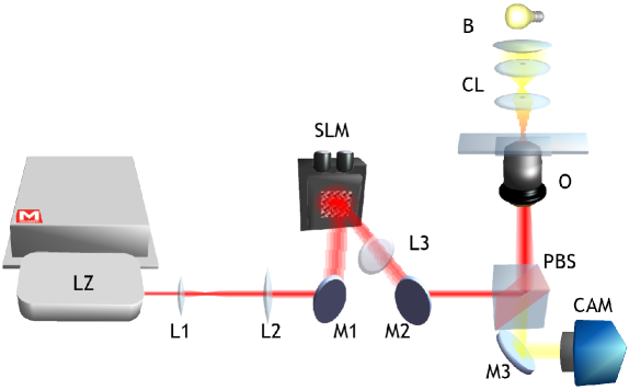
Figure 1: Experimental setup. From left to right. (LZ) Ti:sapphire laser system, (L1 and L2) Beam Telescope, (M1 and M2) Folding Mirrors, (SLM)Boulder Fast SLM,(L3), (PBS) Polarising beam splitter cube, (M3) Mirror, (CAM) Prosilica Fast camera, (O) Objective lens, (CL)Condensing optics, (B) 250W halogen bulb.

Trapping is achieved using a CW Ti:sapphire laser system (M Squared, SolsTiS) which provides up to 1 W at 830 nm. Holographic optical traps are created via the use of a spatial light modulator (Boulder XY series) [8] in the Fourier plane of the optical traps. The tweezers are based around an inverted microscope, where the same objective lens, 100$\times$ 1.3NA, (Zeiss, Plan-Neofluor) is used both to focus the trapping beam and to image the resulting motion of the particles. Samples are mounted in a motorized microscope stage (ASI, MS-2000). Particles are imaged using bright-field illumination. We use a Prosilica GC640M camera to view the trapped particle and our own suite of camera analysis software written in LabVIEW (available from [26]) to measure the position of the trapped particle in real time at up to 2 kHz frame rate [27].

4 Results

The normalized position autocorrelation functions $A(\tau)$, measured from the stochastic fluctuations of beads optically trapped in two different fluids are shown in Fig. 2, together with the function predicted for a simple Newtonian fluid. In the Newtonian case, it is expected that $A(\tau)$ decays as a single exponential with a characteristic relaxation rate related to the trap strength, bead size and fluid viscosity i.e. Eq. (5). The agreement between the data and prediction for water is good. On the other hand, in the case of a non-Newtonian fluid, where the viscosity is time-dependent, it is not guaranteed that Eq. (4) could be resolved (i.e. inverse-Laplace transformed) into a simple form like Eq. (5). However, this is no hindrance since the viscoelastic moduli will be found via the analysis of the normalized position autocorrelation function. In Fig. 3 we compare the impulse response (i.e. step II of the procedure) of a $5\mu m$ diameter bead suspended in water and in an aqueous solution of PAM at 1% w/w (a non-Newtonian fluid), with a duration between flips of $P=20$ s and a trap centre-to-centre separation of $D_{0}=1.6\mu m$, giving $D_{0}/a=0.64$. In order to guarantee the linearity of the confining forces exerted by the two optical traps, the distance between them was always chosen to be no more than 80% of the bead radius, $D_{0}\leq 0.8a$ [1]. Although Brownian statistical fluctuations appear in the figure, the difference between the viscoelastic natures of the two fluids is clear. Indeed, while a bead suspended in water flips from one trap to the other almost instantaneously, the same bead in the PAM solution takes much longer (a few seconds) to flip. In order both to evaluate $D(t)=\left|\left\langle\vec{r}(t)\right\rangle\right|/D_{0}$ and to reduce noise caused by Brownian fluctuations, the transient measurements were averaged over twenty flips, with the resulting curves shown in Figure 4. Experimentally, the switching process of the two traps is controlled by means of a spatial light modulator (SLM) which alternately creates an optical trap in one of two positions. It is important at this point to note that there is a short but finite time for which both traps exist simultaneously [8], due to the finite time required by the SLM’s display to update the holographic pattern. This makes the switching process not exactly binary. However, this will of course only affect the high-frequency results obtained during this step which will ultimately be neglected in favour of the high-frequency response from step (I).

Wideband microrheological measurement are obtained from the optical tweezers by combining the frequency responses obtained from both steps (I) and (II) of the procedure. In particular, the material’s high-frequency response is determined by applying Eq. (7) (via Eq. (2) with $A_{k}$ replacing $g_{k}$) to the $A(\tau)$ measurements (in which low-frequency information tends to be very noisy); whereas, the low-frequency response is resolved by applying Eq. (10) (via Eq. (2) with $D_{k}$ replacing $g_{k}$) to the data describing the bead’s transient response to the flipping traps (in which the high-frequency response is limited by the performance of the SLM).

Typical results for both Newtonian and non-Newtonian fluids are shown in Figures 5 and 6, respectively. In both the cases, it is evident that, although there is some noise in the frequency domain which comes from genuine experimental noise in the time-domain data, there is a clear overlapping region of agreement between the two methods which makes the whole procedure self-consistent. Moreover, it confirms the ease with which the low-frequency material response can be explored right down to the terminal region (where $G^{\prime}\propto\omega^{2}$ and $G^{\prime\prime}\propto\omega$). This is the current limitation for microrheological measurements.

5 Conclusions

In summary, we have presented a self-consistent and simple experimental procedure, coupled with a data analysis methods, for determining the wide-band viscoelastic properties of complex fluids using optical tweezers. This method extends the range of the frequencies previously available to optical tweezers measurements. In fact,the accessible frequency range is limited only by the experiment length and by the maximum data acquisition speed (10s of MHz for a quadrant photo-diode). This allows access to the material’s terminal region enabling micro-rheological measurements to be performed on complex fluids with very long relaxation times, such as those exhibiting soft glassy rheology [28]. The method provides a simple yet concrete basis on which future viscoelastic measurements may be made on both biological and non-biological systems using optical tweezers.

6 ACKNOWLEDGEMENTS

The project was funded by the BBSRC, EPSRC DTC and by BT Grant ”Listening to the microworld“.

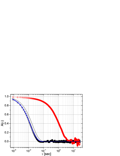
Figure 2: The normalised position autocorrelation function vs. lag-time of a $5\mu m$ diameter bead (squares) in water (with $\kappa=2.7\mu N/m$) and (circles) in a water-based solution of PAM at concentrations of $1$ % $w/w$ (with $\kappa=2.2\mu N/m$). The continuous and dotted lines represent Eq. (5) for a $5\mu m$ diameter bead in water at $T=25^{o}C$ with $\kappa=2.7\mu N/m$ and $\kappa=2.2\mu N/m$, respectively.

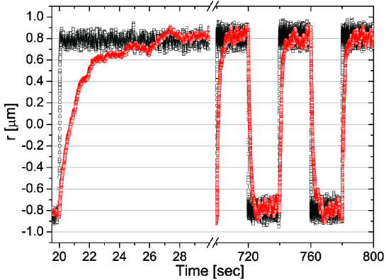
Figure 3: The trajectory of a $5\mu m$ diameter bead flipping between two optical traps $\kappa_{1}$ (bottom) and $\kappa_{2}$ (top) repeatedly switching after a duration $P=20$ s. The bead is suspended in (squares) water (with $\kappa_{1}=2.7$ and $\kappa_{2}=2.5\mu N/m$) and (circles) a water-based solution of PAM at concentrations of $1$ % $w/w$ (with $\kappa_{1}=2.1$ and $\kappa_{2}=2.2\mu N/m$).

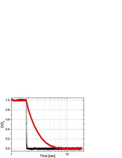
Figure 4: The normilized mean position of all step-down data shown in Fig. 3; i.e., when simultaneously trap 2 (top) switches off and trap 1 (bottom) switches on.

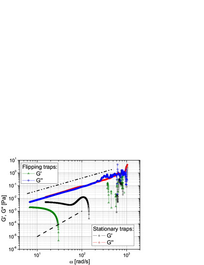
Figure 5: Storage ($G^{\prime}$) and loss ($G^{\prime\prime}$) moduli of water vs. frequency, analysed using both Eq. (7) (high frequencies) and Eq. (10) (low frequencies) applied directly to the experimental data presented in Fig. 2 and Fig. 4, respectively. The lines represents the expected limiting behaviour of the moduli when the material reaches the terminal region: $G^{\prime}\propto\omega^{2}$ and $G^{\prime\prime}\propto\omega$.

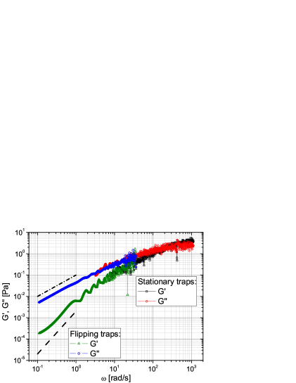
Figure 6: Storage ($G^{\prime}$) and loss ($G^{\prime\prime}$) moduli vs. frequency of a solution of 1% w/w of PAM in water measured by means of both Eq. (7) (high frequencies) and Eq. (10) (low frequencies) applied directly to the experimental data presented in Fig. 2 and Fig. 4, respectively. The lines represents the expected limiting behaviour of the moduli when the material reaches the terminal region: $G^{\prime}\propto\omega^{2}$ and $G^{\prime\prime}\propto\omega$.

References

References

- [1] A. Ashkin. Forces of a single-beam gradient laser trap on a dielectric sphere in the ray optics regime. Biophysical Journal, 61(2):569–582, 1992.
- [2] J.E. Molloy, J.E. Burns, J. Kendrick-Jones, R.T. Tregear, and D.C.S. White. Movement and force produced by a single myosin head. Nature, 378:209–212, 1995.
- [3] S.M. Block, D.F. Blair, and H.C. Berg. Compliance of bacterial flagella measured with optical tweezers. Nature, 338(6215):514–8, 1989.
- [4] J. Guck, R. Ananthakrishnan, H. Mahmood, T. J. Moon, C.C. Cunningham, and J. Kas. The optical stretcher: A novel laser tool to micromanipulate cells. Biophysical Journal, 81(2):767–784, 2001.
- [5] M.D. Wang, H. Yin, R. Landick, J. Gelles, and S.M. Block. Stretching dna with optical tweezers. Biophysical Journal, 72(3):1335–1346, 1997.
- [6] A. Ashkin, J.M. Dziedzic, J.E. Bjorkholm, and S. Chu. Observation of a single-beam gradient force optical trap for dielectric particles. Optics Letters, 11:288–290, 1986.
- [7] E.R. Dufresne, G. Spalding, M. Dearing, S. Sheets, and D.G. Grier. Computer-generated holographic optical tweezers arrays. Review of Scientific Instruments, 72:1816–1820, 2001.
- [8] D. Preece, R. Bowman, A. Linnenberger, G.M. Gibson, S. Serati, and M. J. Padgett. Increasing trap stiffness with position clamping in holographic optical tweezers. Optics Express, 17(25):22718–25, December 2009.
- [9] K. Svoboda, C.F. Schmidt, D. Branton, and S.M. Block. Conformation and elasticity of the isolated red blood cell membrane skeleton. Biophysical Journal, 63(3):784–793, 1992.
- [10] M.E.J. Friese, H. Rubinsztein-Dunlop, and J. Gold. Optically driven micromachine elements. Applied Physics, 2001.
- [11] A. Bishop, T. Nieminen, N. Heckenberg, and H. Rubinsztein-Dunlop. Optical microrheology using rotating laser-trapped particles. Physical Review Letters, 92(19):14–17, 2004.
- [12] J.D. Ferry. Viscoelastic properties of polymers. (Wiley,New York, 1980), 3rd ed., 1980.
- [13] M. Tassieri, G.M. Gibson, R.M.L. Evans, A. M. Yao, R. Warren, M.J. Padgett, and J.M. Cooper. Measuring storage and loss moduli using optical tweezers: Broadband microrheology. Physical Review E, 81(2), 2010.
- [14] K.C. Neuman and S.M. Block. Optical trapping. The Review of Scientific Instruments, 75(9):2787–809, 2004.
- [15] R. Di Leonardo, S. Keen, F. Ianni, J. Leach, M.J. Padgett, and G. Ruocco. Hydrodynamic interactions in two dimensions. Physical Review E, 78(3):31406, 2008.
- [16] K. Berg-Sørensen and H. Flyvbjerg. Power spectrum analysis for optical tweezers. Review of Scientific Instruments, 75(3):594–612, 2004.
- [17] A. Yao, M. Tassieri, M. Padgett, and J.M. Cooper. Microrheology with optical tweezers. Lab on a chip, 9(17):2568–75, 2009.
- [18] L. Starrs and P. Bartlett. One- and two-point micro-rheology of viscoelastic media. Journal of Physics: Condensed Matter, 15(1):S251–S256, 2003.
- [19] M. Atakhorrami, D. Mizuno, G. H. Koenderink, T. B. Liverpool, F. C. MacKintosh, and C. F. Schmidt. Short-time inertial response of viscoelastic fluids measured with brownian motion and with active probes. Physical Review E, 77(6), 2008.
- [20] N. Nijenhuis, D. Mizuno, J. A. E. Spaan, and C.F. Schmidt. Viscoelastic response of a model endothelial glycocalyx. Physical biology, 6(2):25014, 2009.
- [21] Giuseppe Pesce, AC De Luca, G Rusciano, PA Netti, S Fusco, and A Sasso. Microrheology of complex fluids using optical tweezers: a comparison with macrorheological measurements. Journal of Optics A: Pure and Applied Optics, 11(3):34016–34026, 2009.
- [22] I. Tolić-Nørrelykke, E. Munteanu, G. Thon, L. Oddershede, and K. Berg-Sørensen. Anomalous diffusion in living yeast cells. Physical Review Letters, 93(7), 2004.
- [23] T. Mason and D. Weitz. Optical measurements of frequency-dependent linear viscoelastic moduli of complex fluids. Physical Review Letters, 74(7):1250–1253, 1995.
- [24] R.M.L. Evans, M. Tassieri, D. Auhl, and T. A. Waigh. Direct conversion of rheological compliance measurements into storage and loss moduli. Physical Review E, 80(1):0125018–11, 2009.
- [25] T. Mason, K. Ganesan, J. van Zanten, D. Wirtz, and S. Kuo. Particle tracking microrheology of complex fluids. Physical Review Letters, 79(17):3282–3285, 1997.
- [26] Glasgow optics group website.
- [27] G.M. Gibson, J. Leach, S. Keen, A. J. Wright, and M. J. Padgett. Measuring the accuracy of particle position and force in optical tweezers using high-speed video microscopy. Optics Express, 16(19):405–412, 2008.
- [28] S. M. Fielding, P. Sollich, and M. E. Cates. Aging and rheology in soft materials. Journal of Rheology, 44(2):323–369, 2000.