First-Passage Properties of Bursty Random Walks

J. Stat. Mech. P06018 (2010)

Abstract

We investigate the first-passage properties of bursty random walks on a finite one-dimensional interval of length $L$, in which unit-length steps to the left occur with probability close to one, while steps of length $b$ to the right — “bursts” — occur with small probability. This stochastic process provides a crude description of the early stages of virus spread in an organism after exposure. The interesting regime arises when $b/L\lesssim 1$, where the conditional exit time to reach $L$, corresponding to an infected state, has a non-monotonic dependence on initial position. Both the exit probability and the infection time exhibit complex dependences on the initial condition due to the interplay between the burst length and interval length.

I Introduction

We are continually exposed to viruses. Despite these constant biological assaults, the immune system successfully fends off most viruses. Considerable effort has been devoted to modeling the factors that influence whether a person exposed to a particular virus will eventually become ill nowak . Typical theoretical models of viral infections account for the evolution of the number of infected cells, healthy cells, and viruses as a function of the rates of microscopic infection and transmission rates. Such models have provided many useful insights about the dynamics of viral diseases nowak ; perelson .

In this work, we study a toy model — the bursty random walk (Fig. 1) — that captures one of the elements of viral infection dynamics. The position of the walk in one dimension represents the number of active viruses in an organism. Since the immune system constantly kills viruses, they are removed from the body at some specified rate, corresponding to steps to the left in the bursty random walk. However, with a small probability, a virus enters and successfully hijacks a cell, the outcome of which is a burst of a large number of new viruses into the host organism, corresponding to a long step to the right in the model.

When the number of virus particles reaches zero, the organism may be viewed as being free of the disease. Conversely, when the number of viruses reaches a threshold value $L$, the organism can be viewed as either being ill or dead. With this simplistic perspective, being cured or becoming ill is recast as a first-passage problem for the bursty random walk in an interval of length $L$. When the burst length $b$ is small, the walk has a diffusive continuum limit whose first-passage properties are well known vk ; fpp . However, if the burst length is of the order of the system length, this burstiness effects strongly affect the first-passage characteristics. This large-burst limit should be applicable to infectious processes where the threshold number of viruses for being ill is not large and the number of new viruses created in a burst event is a finite fraction of this threshold PKP10 . Related discreteness effects were found in the first-passage characteristics of a random walk that hops uniformly within a range $[-a,a]$ in the interval $[0,L]$, with $a\lesssim L$ AR06 .

Figure 1: A bursty random walk with burst length $b=6$.

In the next section, we define the model and the basic first-passage quantities that we will investigate. In Secs. III and IV, we determine the exit probabilities and the average exit times to either end of the interval as a function of the burst length $b$. When $b\lesssim L$, very different first-passage properties arise compared to those for pure diffusion in the interval. Perhaps the most striking is the conditional exit time to reach $x=L$, corresponding to a state of infection, which has a non-monotonic dependence on the starting position $x$. We compute these first-passage properties from the backward Kolmogorov equations for the exit probabilities and exit times vk ; fpp . In the concluding section, we briefly discuss the corresponding first-passage properties for the bursty birth/death model. This process accounts for the feature that bursts should occur at a rate that is proportional to the number of live viruses. It is naturally to model this situation by defining the rate at which steps occur to be proportional to the current position of a bursty walk on the interval.

II The Model

In the bursty random walk, unit-length steps to the left occur with probability $q$, while long steps (bursts) of length $b$ occur with probability $p=1-q$ (Fig. 1). We choose $p$ and $q$ so that the average position of the walk does not change at each step; however, most of our results are derived for general $p$ and $q$. The motivation for considering these hopping probabilities is based on the experimental observation that viral counts in an organism often remain nearly constant for time periods much longer than the lifetime of individual viruses. Such a near constancy could only arise if an organism produces new viruses (by bursts) and clears viruses at similar overall rates perelson .

With the constraint that the number of virus particles remains fixed, on average, the respective probabilities of making a single step to the right and to the left are

$$p=\frac{1}{b+1}~{},\qquad\qquad q=\frac{b}{b+1}~{}.$$ (1)

The bursty random walk is confined to the finite interval $[0,L]$, where the coordinate represents the number of live viruses. The state where the virus is cleared is represented by the point $x=0$, while the state where a sufficient number of viruses exists that the organism is ill or dead is represented by $x=L$. Our goal is to understand first-passage properties of this bursty walk that are relevant to the state of health of the organism. Namely, what is the probability that the organism becomes cured or becomes ill, corresponding to the walk eventually exiting through the left edge or the right edge of the interval, respectively? What is the time needed for the organism to become cured or ill?

To set the stage for our results, let us recall some well-known first-passage properties for the isotropic nearest-neighbor random walk on the interval fpp . Let $\mathcal{E}_{+}(x)$ denote the probability that this random walk eventually exits the interval at $L$ without ever touching $x=0$, given that the walk started at an arbitrary point $x$, with $0<x<L$. The complementary exit probability to the left boundary is $\mathcal{E}_{-}(x)=1-\mathcal{E}_{+}(x)$. These exit probabilities satisfy the recursion

$$\mathcal{E}_{\pm}(x)=\tfrac{1}{2}\,\mathcal{E}_{\pm}(x-1)+\tfrac{1}{2}\,\mathcal{E}_{\pm}(x+1)\,,$$ (2)

subject to the boundary conditions $\mathcal{E}_{+}(0)=0,~{}\mathcal{E}_{+}(L)=1$, or $\mathcal{E}_{-}(0)=1,~{}\mathcal{E}_{-}(L)=0$. This recursion expresses the exit probability starting at $x$ as the probability of first taking a step to the left or right (the factor 1/2) and then exiting from either $x-1$ or $x+1$, respectively. The solution to Eq. (2) with these boundary conditions is:

$$\mathcal{E}_{+}(x)=\frac{x}{L}~{},\qquad\mathcal{E}_{-}(x)=1-\frac{x}{L}~{}.$$ (3)

We also define $t(x)$ as the average time for the walk to leave the interval at either end when it starts at $x$. This unconditional exit time satisfies the recursion

$$t(x)=\tfrac{1}{2}\,t(x-1)+\tfrac{1}{2}\,t(x+1)+1\,,$$ (4)

subject to the boundary conditions $t(0)=t(L)=0$. Equation (4) expresses the average exit time from $x$ as the time for the first step (the additive factor 1) plus the exit time from the new positions (either $x\pm 1$); the factor $\frac{1}{2}$ accounts for the probability for each of these two choices. Similarly, we also define the conditional exit times, $t_{\pm}(x)$, as the average times for the walk to leave the interval by the right or the left boundary, respectively, without ever reaching the opposite boundary. These conditional exit times satisfy fpp

$$\mathcal{C}_{\pm}(x)=\tfrac{1}{2}\,\mathcal{C}_{\pm}(x\!-\!1)+\tfrac{1}{2}\,\mathcal{C}_{\pm}(x\!+\!1)+\mathcal{E}_{\pm}(x)\,,$$ (5)

with $\mathcal{C}_{\pm}\equiv\mathcal{E}_{\pm}t_{\pm}$, and this equation is subject to the boundary conditions $\mathcal{C}_{\pm}(0)=\mathcal{C}_{\pm}(L)=0$. For the nearest-neighbor random walk, the exit times are given by

$$\begin{split}t(x)&=\tfrac{1}{2}\,x(L-x)\,,\\ t_{+}(x)&=\tfrac{1}{3}(L^{2}-x^{2})\,,\\ t_{-}(x)&=\tfrac{1}{3}(2Lx-x^{2})\,.\end{split}$$ (6)

Our goal is to determine the results analogous to Eqs. (3) and (6) for the bursty random walk. As we shall see, first-passage properties depend only on $b/L$ as long as this ratio is nonzero.

III Exit Probabilities

For the bursty random walk with burst length $b$, we may naturally define two distinct types of exit probabilities to the right boundary:

• the total exit probability $\mathcal{E}_{+}(x)$ that the walk eventually reaches any point at the right boundary or beyond, without ever touching the left boundary $x=0$;

• the restricted exit probability $\mathcal{R}_{m}(x)$ that the walk eventually reaches the specific point $L+m$ (with $0\leq m\leq b-1$), without ever touching the left boundary or any other point beyond the right boundary. There are $b$ such distinct restricted exit probabilities, $\mathcal{R}_{m}(x)$, with $m=0,1,\ldots,b-1$.

While the total exit probability is most relevant physically, because it corresponds to the probability of illness for a given level of initial exposure, the restricted exit probabilities display intriguing features that stem from the bursty character of the walk left .

The total exit probability to the right boundary satisfies the recursion

$$\mathcal{E}_{+}(x)=q\mathcal{E}_{+}(x-1)+p\mathcal{E}_{+}(x+b)\,,$$ (7)

that represents the extension of Eq. (2) to the bursty random walk. This recursion expresses exit via the right boundary, when starting from $x$, either by taking the first step to the left (probability $q$), after which exit from $x-1$ occurs, or by first stepping to the right (probability $p$), after which exit from $x+b$ may occur. This recursion must be supplemented by the boundary conditions $\mathcal{E}_{+}(x)=1$ for all $x\geq L$ and $\mathcal{E}_{+}(0)=0$. Namely, a walk that starts at $x\geq L$ has already exited, while a walk that starts at $x=0$ can never exit via the right boundary. The equations for the restricted exit probabilities are similar to (7), but are now subject to the boundary conditions $\mathcal{R}_{m}(0)=0$ and $\mathcal{R}_{m}(L+k)=\delta_{k,m}$.

While the exit probabilities can be obtained by enumerating all random walk trajectories to the exit point and computing the probabilities for all these paths, the above recursions provide the same results much more easily vk ; fpp . We will use different methods to solve Eqs. (7) for short and large burst lengths, and therefore study these cases separately.

III.1 Burst lengths $b=2,3,\ldots$

For the first non-trivial case of burst length $b=2$, we solve the constant-coefficient recursion (7) by attempting a solution of the form ${E}_{+}(x)=\lambda^{x}$. This leads to the characteristic equation $\lambda^{3}-3\lambda+2=0$, with solutions $\lambda=-2$ and $\lambda=1$ (doubly degenerate). Henceforth, we use $\lambda$ to denote the first root of the characteristic polynomial. The general solution to Eq. (7) thus is $\mathcal{E}_{+}(x)=a\lambda^{x}+bx+c$. Invoking the boundary conditions, the total exit probability to the right boundary is

$$\mathcal{E}_{+}(x)=\frac{x}{L\!+\!1}+\frac{1}{L\!+\!1}\frac{\left[(\lambda^{x}\!-\!1)-\frac{x}{L+1}(\lambda^{L+1}\!-\!1)\right]}{\left[(\lambda^{L}\!-\!1)-\frac{L}{L+1}(\lambda^{L+1}\!-\!1)\right]}~{}.$$ (8)

For the restricted exit probabilities to a specific point in the range $[L,L+b-1]$, the boundary conditions are:

$$\mathcal{R}_{0}(0)\!=\!\mathcal{R}_{0}(L\!+\!1)\!=\!0,~{}\mathcal{R}_{0}(L)\!=\!1,~{}\mathrm{exit\ to\ }x=L,$$

$$\mathcal{R}_{1}(0)\!=\!\mathcal{R}_{1}(L)\!=\!0,~{}\mathcal{R}_{1}(L\!+\!1)\!=\!1\,~{}~{}\mathrm{exit\ to\ }x=L\!+\!1.$$

Applying these boundary conditions to the general solution $a\lambda^{x}+bx+c$, we obtain

$$\begin{split}\mathcal{R}_{0}(x)&=\frac{(\lambda^{x}-1)-\frac{x}{L+1}(\lambda^{L+1}-1)}{(\lambda^{L}-1)-\frac{L}{L+1}(\lambda^{L+1}-1)}~{},\\ \mathcal{R}_{1}(x)&=\frac{(\lambda^{x}-1)-\frac{x}{L}(\lambda^{L}-1)}{(\lambda^{L+1}-1)-\frac{L+1}{L}(\lambda^{L}-1)}~{},\end{split}$$ (9)

for the restricted exit probabilities to $x=L$ and to $x=L+1$, respectively. Parenthetically, once we know one of $\mathcal{R}_{0}(x)$ or $\mathcal{R}_{1}(x)$, the other is determined by the martingale property that the mean position of the bursty walk always remains fixed GS01 . That is, after all the probability has reached an absorbing boundary, the two restricted exit probabilities are related by $0\times[1-\mathcal{R}_{0}(x)-\mathcal{R}_{1}(x)]+L\times\mathcal{R}_{0}(x)+(L+1)\times\mathcal{R}_{1}(x)=x$. The restricted exit probabilities initially grow nearly linearly in $x/L$ (Fig. 2), but then oscillate violently as $x\to L$. The total exit probability $\mathcal{E}_{+}(x)$ is a nearly linear function of $x$ for small $x$ but its slope develops oscillations as $x\to L$.

This same calculational method can be extended to longer bursts. By assuming an exponential solution of the form $\mathcal{E}_{+}(x)=\lambda^{x}$ in Eq. (7), the characteristic polynomial generically is $(\lambda-1)^{2}A(\lambda)$, where $A(\lambda)$ is a polynomial of order $b-1$. Explicit closed-form solutions can therefore be obtained for $b\leq 5$, but numerically exact results can be obtained for any burst length; details for the case $b=3$ are given in appendix A. Typical results are shown in Fig. 2 for burst lengths $b=2$, 10, and also $b=\frac{L}{3}$, $\frac{L}{2}$, and $L$. The total exit probability is very close to linear function with slope less than one for $x<L-b$, but deviates from linearity within one burst length from $x=L$. The restricted exit probabilities are also nearly linear functions for $x<L-b$, but oscillate violently in the boundary region.

III.2 Long Bursts

When the burst length is of the order of the interval length, we can simplify the determination of the exit probabilities by considering separate recursions in each of the disjoint subintervals $[L-b,L]$, $[L-2b,L-b-1]$, $[L-3b,L-2b-1]$, etc., instead of directly solving for the roots of a characteristic polynomial of order $b-1$. As we shall see, this partitioning significantly reduces the order of the recursions for the exit probabilities.

III.2.1 Total exit probabilities

In the extreme situation where the burst length $b\geq L$, a single burst results in exit at or beyond the right end of the interval. Thus the total exit probability satisfies the recursion $\mathcal{E}_{+}(x)=q\mathcal{E}_{+}(x-1)+p$; that is, either the walk steps to the left and then exits from $x-1$, or the walk steps to the right and exits immediately. The solution to this recursion is a constant plus an exponential function. The boundary condition $\mathcal{E}_{+}(0)=0$ immediately gives

$$\mathcal{E}_{+}(x)=1-q^{x}.$$ (10)

Because of the overwhelming probability of stepping to the left, the exit probability to the right boundary is not close to one for $x\to L$ from below. As an example, for $b=L$, we have $\mathcal{E}_{+}(L-1)\to 1-e^{-1}\approx 0.6321$ (Fig. 2(c)).

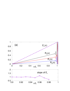
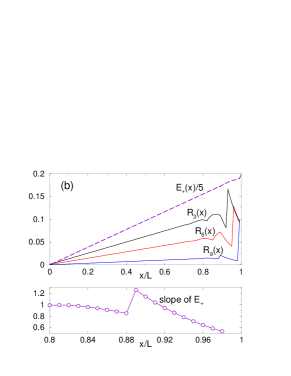
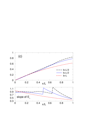
Figure 2: Exit probabilities for the bursty random walk for: (a) burst length $b=3$, (b) $b=10$, and (c) $b=L$, $L/2$, and $L/3$. Simulations are on a system of length $L=100$.

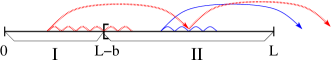
Figure 3: Partitioning of the interval into $[0,L-b-1]$ (region I) and $[L-b,L]$ (region II). To exit from region I requires at least two bursts.

For the case $L/2\leq b<L$, we partition $[0,L]$ into the subintervals $[0,L-b-1]$ (defined as region I) and $[L-b,L]$ (region II), as indicated in Fig. 3. Making a slight abuse of notation, we define $\mathcal{E}^{\rm I}(x)$ and $\mathcal{E}^{\rm II}(x)$ as the total exit probabilities to $x\geq L$, when starting at a point $x$ that is in either region I or region II, respectively. These exit probabilities satisfy

$$\begin{split}\mathcal{E}^{\rm I}(x)&=q\mathcal{E}^{\rm I}(x-1)+p\mathcal{E}^{\rm II}(x+b)\,,\\ \mathcal{E}^{\rm II}(x)&=q\mathcal{E}^{\rm II}(x-1)+p\,.\end{split}$$ (11)

These recursions are identical in form to Eqs. (7), but with the subinterval explicitly identified. Thus, from example, exit to $x\geq L$, when starting from a point $x$ in region I, can occur by taking a step to the left with probability $q$ and then exiting from $x-1$ (necessarily in region I), or by taking a step to the right with probability $p$ and then exiting from $x+b$ (necessarily in region II). Equations (11) are subject to the boundary condition $\mathcal{E}^{\rm I}(0)=0$ as well as the joining condition $\mathcal{E}^{\rm II}(L-b)=q\mathcal{E}^{\rm I}(L-b-1)+p$.

By this partitioning, the exit probabilities in each subinterval are functionally distinct and can be solved separately. In the second of Eqs. (11), a particular solution is $\mathcal{E}^{\rm II}_{\rm par}=1$. Thus the general solution has the form $\mathcal{E}^{\rm II}(x)=1+Aq^{x}$. Substituting this expression in the first of Eqs. (11), now gives the closed recursion $\mathcal{E}^{\rm I}(x)=q\mathcal{E}^{\rm I}(x-1)+p+Apq^{x}$. With the inhomogeneous term $p+Apq^{x}$, the general solution is $\mathcal{E}^{\rm I}(x)=A+(Bx+C)q^{x}$. Using the boundary condition $\mathcal{E}^{\rm I}(0)=0$, and substituting this form for $\mathcal{E}^{\rm I}(x)$ into the first of Eqs. (11), we find $B=Apq^{b}$. Finally, we invoke the joining condition and obtain

$$\mathcal{E}^{\rm I}(x)=1\!-\!q^{x}-\frac{x\,p\,q^{x+b}}{1\!-\!ypq^{b}}~{},\quad\mathcal{E}^{\rm II}(x)=1\!-\!\frac{q^{x}}{1\!-\!ypq^{b}}~{},$$ (12)

where $y\equiv L-b-1$. Notice again that because of the large probability of hopping to the left, $\mathcal{E}_{\rm II}(x)$ is discontinuous as $x\to L$.

For $L/3\leq b<L/2$, we partition $[0,L]$ into the three subintervals $[0,L-2b-1]$, $[L-2b,L-b-1]$, and $[L-b,L]$, (regions I, II, and III respectively) and solve the generalization of Eqs. (11) to three intervals, supplemented by two joining conditions at $x=L-b$ and at $x=L-2b$ (appendix B). As shown in Fig. 2, the total exit probability has two (barely visible) singularities and deviates considerably from linearity within one burst length from the right boundary. Generally, for a partitioning into $k$ intervals, the slope of the total exit probability is discontinuous at the boundary between intervals $k$ and $k-1$, the second derivative is discontinuous at the boundary between intervals $k-1$ and $k-2$, the third derivative is discontinuous at the boundary between intervals $k-2$ and $k-3$, etc. A similar intricate pattern of a sequence of progressively weaker singularities arises in various fragmentation models DF87 ; FIK95 .

III.2.2 Restricted exit probabilities

The restricted exit probabilities to a specific point undergo a more dramatic sequence of discontinuities between successive subintervals. We again start with the case where $b$ lies in the range $[L/2,L]$ so that there are two subintervals to consider: $[0,L-b-1]$ and $[L-b,L]$. For concreteness we determine the exit probability to the specific site $x=L$; similar behavior arises for other exit points in $[L,L+b-1]$. Now the recursion relations for the restricted exit probabilities are

$$\begin{split}\mathcal{R}^{\rm I}(x)&=q\mathcal{R}^{I}(x-1)+p\mathcal{R}^{\rm II}(x+b)\,,\\ \mathcal{R}^{\rm II}(x)&=q\mathcal{R}^{\rm II}(x-1)\,.\end{split}$$ (13)

Since we seek only the exit probability to $x=L$, we simplify notation by omitting the subscript that specifies the exit location; thus $\mathcal{R}_{0}\to\mathcal{R}$. The first equation states that to reach $x=L$ from subinterval I, the walk can either step left (probability $q$) and exits from $x-1$, or the walk steps to the right (probability $p$) and exits from $x+b$. The second equation states that to reach $x=L$ from within subinterval II, the only possibility is to step to the left; a burst would lead to exit at a point $x>L$, which does do not contribute to the exit probability to $x=L$. The recursions (13) must be supplemented by the boundary condition $\mathcal{R}^{\rm I}=0$ and the joining condition $\mathcal{R}^{\rm II}(L-b)=q\mathcal{R}^{\rm I}(L-b-1)+p$. Notice that exit to $L$ can occur only if the walk is at the point $x=L-b$.

 

Figure 4: Restricted exit probabilities to $x=L$ for the cases of $b=L/2$ and $b=L/3$. The arbitrary vertical scale has been fixed by setting the integral of $\mathcal{R}(x)$ over the interval equal to 1.

Employing the same method as that used to obtain Eqs. (12), we now obtain obtain

$$\mathcal{R}^{\rm I}(x)=\frac{xp^{2}q^{x+2b-L}}{1-ypq^{b}}~{},\qquad\mathcal{R}^{\rm II}(x)=\frac{pq^{x+b-L}}{1-ypq^{b}}~{}.$$ (14)

This solution method can be extended to more subintervals; the results for $b=L/2$ (two intervals) and $b=L/3$ (three intervals) are shown in Fig. 4. For a partitioning into $k$ intervals, the exit probability is discontinuous at the boundary between intervals $k$ and $k-1$, the first derivative is discontinuous at the boundary between intervals $k-1$ and $k-2$, etc.; the pattern is similar to that for the total exit probability, but the discontinuities are more prominent here since they begin with the function itself rather than with the first derivative.

IV First-Passage Times

By adapting Eq. (4) to the bursty random walk, the unconditional mean first-passage time satisfies

$$t(x)=qt(x\!-\!1)+pt(x\!+\!b)+1\,,$$ (15)

subject to the boundary conditions $t(0)=0$ and also $t(L\!+\!m)=0$ for $m=0,1,\ldots b-1$. Similarly, the quantities $\mathcal{C}_{\pm}(x)$, which are related to the conditional exit times, satisfy the recursion (see Eq. (5))

Similarly, the conditional mean first-passage times $\mathcal{C}_{\pm}(x)$ satisfy the recursion (see Eq. (5))

$$\mathcal{C}_{\pm}(x)=q\mathcal{C}_{\pm}(x\!-\!1)+p\mathcal{C}_{\pm}(x\!+\!b)+\mathcal{E}_{\pm}(x)\,,$$ (16)

subject to the same boundary conditions as for $t(x)$ itself. Again, we treat the exit times separately for short and for long bursts.

IV.1 Short bursts

For the first non-trivial case of $b=2$, let us focus on the unbiased case of $p=\frac{1}{3}$ and $q=\frac{2}{3}$ for simplicity. We solve the recursion (15) with these values of $p$ and $q$ by noting that the inhomogeneous term can be eliminated by writing $t(x)=T(x)-x^{2}/2$. Substituting this ansatz into Eq. (15), we find that $T(x)$ obeys this same equation, but without the inhomogeneous term. From our analysis of the exit probability in Sec. III.1, the general solution is $T(x)=a\lambda^{x}+bx+c$, with $\lambda=-2$, subject to the boundary conditions $T(0)=0$, $T(L)=L^{2}/2$, $T(L+1)=(L+1)^{2}/2$ that correspond to $t(0)=t(L)=t(L+1)=0$. We thereby obtain, for the unconditional mean first-passage time,

$$t(x)=\frac{1}{2}x(L\!-\!x)+\frac{1}{2}\frac{(L\!+\!1)\big{[}(\lambda^{x}\!-\!1)-\frac{x}{L}(\lambda^{L}\!-\!1)\big{]}}{(\lambda^{L+1}-1)-\frac{L+1}{L}(\lambda^{L}\!-\!1)}~{},$$ (17)

with $\lambda=-2$. The second term represents a tiny correction to the leading diffusive behavior of $\frac{1}{2}x(L-x)$.

IV.2 Long Bursts

In the extreme case of burst length $b\geq L$, the walk exits after any single burst, and the unconditional first-passage time satisfies $t(x)=qt(x-1)+1$, subject to the boundary condition $t(0)=0$. The solution is

$$t(x)=\frac{1-q^{x}}{1-q~{}}~{}.$$ (18)

Similarly, the conditional mean first-passage time to the right boundary, $t_{+}=\mathcal{C}_{+}/\mathcal{E}_{+}$, is determined from the recursion

$$\mathcal{C}_{+}(x)=q\mathcal{C}_{+}(x-1)+\mathcal{E}_{+}(x)=q\mathcal{C}_{+}(x-1)+1-q^{x}\,,$$ (19)

subject to the boundary condition $\mathcal{C}_{+}(0)=0$. The solution now is

$$t_{+}(x)=\frac{1}{1-q}-\frac{x\,q^{x}}{1-q^{x}}~{}.$$ (20)

The conditional exit time $t_{-}$ may be obtained from the conservation statement $t(x)=\mathcal{E}_{-}(x)t_{-}(x)+\mathcal{E}_{+}(x)t_{+}(x)$ and gives $t_{-}(x)=x$. An apparently paradoxical feature is that the exit time $t_{+}$ increases when the starting point is closer to $x=L$ (Fig. 5(d)). This behavior arises because steps to the left occur with overwhelming probability. Thus a walk that starts near $x=L$ will almost surely hop a considerable distance to the left before a burst occurs. However a walk that starts near $x=0$ can only hop a short distance to the left before a burst must occur to ensure exit at the right boundary.

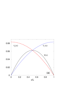
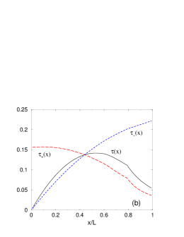
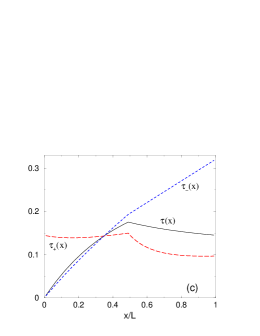
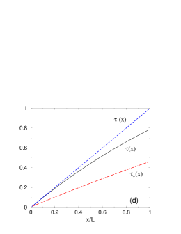
Figure 5: Normalized mean first-passage times $\tau\equiv t/(L^{2}\!/\!D)$, with $D=b/2$, for: (a) the nearest-neighbor random walk, and the bursty random walk with: (b) burst length $b=L/5$, (c) $b=L/2$, and (d) $b=2L$. Shown are the unconditional first-passage time $\tau(x)$ and the conditional times, $\tau_{\pm}(x)$, to the right and left boundary, respectively.

For $L/2\leq b<L$, we again partition the interval into the subintervals $[0,L-b-1]$ (region I) and $[L-b,L]$ (region II) and denote the mean first-passage times within each as $t^{\rm I}(x)$ and $t^{\rm II}(x)$ respectively. The unconditional mean first-passage time satisfies

$$\begin{split}t^{\rm I}(x)&=qt^{\rm I}(x-1)+pt^{\rm II}(x+b)+1\,,\\ t^{\rm II}(x)&=qt^{\rm II}(x-1)+1\,,\end{split}$$ (21)

subject to the boundary condition $t^{\rm I}(x)=0$ and the joining condition $t^{\rm II}(L-b)=qt^{\rm I}(L-b-1)+1$. Solving first for $t^{\rm II}$ and then using this solution in the equation for $t^{\rm I}$, we obtain

$$\begin{split}t^{\rm I}(x)&=\frac{x\left(q^{-y}-2\right)q^{b+x}}{1-ypq^{b}}-\frac{2\left(q^{x}-1\right)}{p}~{},\\ t^{\rm II}(x)&=\frac{\left(1-ypq^{b}+q^{x-y}-2q^{x}\right)}{p\left(1-ypq^{b}\right)}~{},\end{split}$$ (22)

with $y=L-b-1$.

For the conditional first-passage time to the right boundary, the quantity $\mathcal{C}_{+}(x)=\mathcal{E}_{+}(x)t_{+}(x)$ satisfies

$$\begin{split}\mathcal{C}^{\rm I}(x)&=q\mathcal{C}^{\rm I}(x-1)+p\mathcal{C}^{\rm II}(x+b)+\mathcal{E}^{\rm I}(x)\,,\\ \mathcal{C}^{\rm II}(x)&=q\mathcal{C}^{\rm I}(x-1)+\mathcal{E}^{\rm II}(x)\,,\end{split}$$ (23)

subject to the boundary condition $\mathcal{C}^{\rm I}(x)=0$ and the joining condition $\mathcal{C}^{\rm II}(L-b)=q\mathcal{C}^{\rm I}(L-b-1)+\mathcal{E}^{\rm II}(L-b)$. Again, we have made the notational abuse of dropping the subscript $\pm$ and focusing only on the exit time to the right boundary. Solving these equations for $\mathcal{C}_{+}$ and dividing by $\mathcal{E}_{+}(x)$ yields the conditional first-passage time to the right boundary (Fig. 5). This same calculation can be straightforwardly (but tediously) extended to smaller values of $b$, corresponding to more subintervals.

Figure 6: The normalized conditional exit time to the right boundary, $\tau_{+}\equiv t_{+}/(L^{2}\!/\!D)$ for the case $b/L=0.8$.

A peculiar feature of the conditional first-passage time $t_{+}(x)$ is its non-monotonic dependence on $x$ as the burst length becomes of the order of the system length (Fig. 6). This non-monotonicity has a simple origin. For $x/L\lesssim 1$, a typical walk will move a considerable distance to the left before exit occurs. Thus, in some sense, points near the right boundary are “further” from the exit than points in the interior of the interval. Similarly, a particle that starts near $x=0$ must quickly hop to the right to avoid exiting at the left boundary. Thus again, the exit time to the right is an increasing function of $x$ in this range. Finally, for a particle that starts in a narrow range in which $x$ is slightly larger than $L-b$, the exit time decreases as $x$ increases. The source of this decreasing dependence on $x$ in this range is that a particle with $x\gtrsim L-b$ is increasingly likely to reach a point that is less than $L-b$ as $x$ decreases toward $L-b$. Once the point $x=L-b$ is crossed, two bursts are required for exit to the right and typically there will be many steps to the left between these two bursts. Thus the exit time increases rapidly as the starting point approaches $L-b$ from above.

V Discussion

We investigated the first-passage properties of the bursty random walk on a finite interval, where short steps to the left occur with a high probability, while long steps to the right — “bursts” — occur with a small probability. The disparity in these hopping probabilities is needed to ensure that there is no net displacement of a random walker, a feature that maximizes the time for the walker to survive within the interval. This model was motivated by the problem of the early stages of virus spread after initial exposure PKP10 .

When the burst length is short, there are only small corrections to the well-known first-passage properties of the nearest neighbor random walk. Conversely, when the burst length is of the order of the interval length, discreteness effects play an important role. For such burst lengths, we solved for first-passage properties by partitioning the full interval into disjoint subintervals of length $b$, solving each one separately, and then patching together these subinterval solutions by invoking appropriate joining conditions. Strikingly, the mean first-passage time to the right boundary, corresponding to the time for a host organism to become ill, has a non-monotonic dependence on the initial location for $b/L\lesssim 1$ (Fig. 6). Another basic feature of the first-passage properties for large $b$ is that they are functions of $b/L$ rather then depending on $b$ and $L$ separately.

In spite of the strange behavior of the mean first-passage time, the distribution of first-passage times is generically characterized by an exponential decay, but with superimposed oscillations due to burstiness. Consequently, higher moments of the first-passage times can be simply characterized by powers of the first moment.

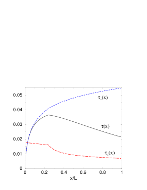
Figure 7: The normalized unconditional and conditional exit times, $\tau\equiv t/L$, for the bursty birth/death process with $b/L=0.75$.

If one takes seriously the equivalence that the position of the random walker as equivalent to the number of active viruses, then the frequency of bursts as well as the frequency of virus death events should also be proportional to the current position of the walk. Thus it would be more realistic to consider the bursty birth/death process, where the rate at which the random walker hops is proportional to its current location. If a step does occur, then a unit-length step to the left occurs with probability $q$ and a step of length $b$ to the right occurs with probability $p\ll q$.

Because the exit probabilities are independent of the rate at which steps occur, all our results about exit probabilities continue to hold for the bursty birth/death process. However, exit times for bursty birth/death are quite different from those of the bursty random walk. For example, the unconditional exit time for bursty birth/death satisfies the recursion

$$t(x)=qt(x-1)+qt(x+b)+\delta t(x)\,,$$ (24)

where $\delta t(x)$, the microscopic time step at position $x$, is proportional to ${1}/{x}$. For the classic birth/death process (burst length $b=1$) and in the continuum limit, Eq. (24) becomes $t^{\prime\prime}(x)=-{2}/{x}$ with solution $t(x)=2x\ln(L/x)$. Over most of the interval range, this exit time scales linearly with $L$, compared to $t(x)\sim L^{2}$ for the exit time of the nearest-neighbor random walk. For bursty birth/death, representative results for exit times are given in Fig. 7. While no longer non-monotonic in $x$, the conditional exit time $t_{+}(x)$ has a near plateau when the initial position $x<L-b$ and then decreases in $x$. Thus once an infection has progressed to a certain threshold, illness quickly ensues.

We thank Paul Krapivsky, John Pearson, and Alan Perelson for useful advice. We also gratefully acknowledge financial support from NSF grant DMR0906504.

Appendix A Exit probabilities for burst length $b=3$

For burst length $b=3$, the recursion relation for the total exit probability to the right boundary is

$$\mathcal{E}_{+}(x)=\tfrac{3}{4}\mathcal{E}_{+}(x-1)+\tfrac{1}{4}\mathcal{E}_{+}(x+3)\,.$$ (25)

Assuming the exponential form $\mathcal{E}_{+}=\lambda^{x}$ and substituting into (25), the characteristic equation is $\lambda^{4}-4\lambda+3=0$, with solutions $\lambda=1$ (doubly degenerate) and $\lambda_{\pm}=-1\pm i\sqrt{2}\equiv\sqrt{3}\,e^{i\phi}$, with $\phi=\tan^{-1}(-\sqrt{2})$. The general solution is $\mathcal{E}_{+}(x)=a\lambda_{+}^{x}+b\lambda_{-}^{x}+cx+d$. Now we impose the boundary conditions $\mathcal{E}_{+}(0)=0$ and $\mathcal{E}_{+}(L)=\mathcal{E}_{+}(L+1)=\mathcal{E}_{+}(L+2)=1$ one by one. The boundary condition $\mathcal{E}_{+}(0)=0$ gives

$$\mathcal{E}_{+}(x)=a(\lambda_{+}^{x}-1)+b(\lambda_{-}^{x}-1)+cx\,.$$ (26)

The boundary condition $\mathcal{E}_{+}(L)=1$ gives

$$\mathcal{E}_{+}(x) = a\left[(\lambda_{+}^{x}-1)-(\lambda_{+}^{L}-1)\frac{x}{L}\right]+b\left[(\lambda_{-}^{x}-1)-(\lambda_{-}^{L}-1)\frac{x}{L}\right]+\frac{x}{L}~{},$$ (27)

$$\equiv a\alpha(x)+b\alpha^{*}(x)+\frac{x}{L}~{},$$

with $\alpha(L)=0$. Next we impose $\mathcal{E}_{+}(L+1)=1$ to give

$$\mathcal{E}_{+}(x) = a\big{[}\alpha(x)\alpha^{*}(L+1)-\alpha^{*}(x)\alpha(L+1)\big{]}+\frac{x}{L}+\left(1-\frac{x}{L}\right)\frac{\alpha^{*}(x)}{\alpha^{*}(L+1)}~{},$$ (28)

$$\equiv aW(x,L+1)+\frac{x}{L}+\left(1-\frac{x}{L}\right)\frac{\alpha^{*}(x)}{\alpha^{*}(L+1)}~{},$$ (29)

where the Wronskian $W(L+1,L+1)=0$. Finally, imposing $\mathcal{E}_{+}(L+2)=1$ gives

$$\mathcal{E}_{+}(x)=\frac{W(x,L+1)}{W(L+2,L+1)}\left[1-\frac{L+2}{L}-\frac{1}{L}\frac{\alpha^{*}(L+2)}{\alpha^{*}(L+1)}\right]+\left[\frac{x}{L}-\frac{1}{L}\frac{\alpha^{*}(x)}{\alpha^{*}(L+1)}\right]~{}.$$ (30)

By inspection, it is clear that Eq. (30) satisfies all the boundary conditions; this solution is also real.

A similar calculation can be performed for all the restricted exit probabilities. For example, for the restricted exit probability $\mathcal{R}_{0}(x)$ to $L$, we start with Eq. (26) and next impose $\mathcal{R}_{0}(L+1)=0$ to give

$$\mathcal{R}_{0}(x) = a\left[(\lambda_{+}^{x}-1)-(\lambda_{+}^{L+1}-1)\frac{x}{L+1}\right]+b\left[(\lambda_{-}^{x}-1)-(\lambda_{-}^{L+1}-1)\frac{x}{L+1}\right]~{},$$ (31)

$$\equiv a\beta(x)+b\beta^{*}(x),$$

with $\beta(L+1)=0$. The boundary condition $\mathcal{R}_{0}(L+2)=0$ leads to $\mathcal{R}_{0}(x)=aV(x,L+2)$, where the Wronskian is now defined as $V(x,y)=\beta(x)\beta^{*}(y)-\beta^{*}(x)\beta(y)$. Imposing the boundary condition $\mathcal{R}_{0}(L)=1$ gives the final result

$$\mathcal{R}_{0}(x)=\frac{V(x,L+2)}{V(L,L+2)}~{}.$$ (32)

For the other two restricted exit probabilities, the same calculation as that outlined above gives

$$\mathcal{R}_{1}(x)=\frac{W(x,L+2)}{W(L+1,L+2)}~{},\qquad\qquad\mathcal{R}_{2}(x)=\frac{W(x,L+1)}{W(L+2,L+1)}~{}.$$ (33)

These results for the total and restricted exit probabilities are plotted in Fig. 2.

Appendix B Exit probabilities for burst length $L/3<b<L/2$

When the burst length $b$ is in the range $[\frac{L}{3},\frac{L}{2}]$, the interval naturally divides into the three subintervals $[0,L-2b-1]$, $[L-2b,L-b-1]$, and $[L-b,L]$. The recursion relations satisfied by the total exit probability to the right edge of the interval are:

$$\begin{split}\mathcal{E}^{\rm I}(x)&=q\mathcal{E}^{\rm I}(x-1)+p\mathcal{E}^{\rm II}(x+b)\,,\\ \mathcal{E}^{\rm II}(x)&=q\mathcal{E}^{\rm II}(x-1)+p\mathcal{E}^{\rm III}(x+b)\,,\\ \mathcal{E}^{\rm III}(x)&=q\mathcal{E}^{\rm III}(x-1)+p\,.\end{split}$$ (34)

These exit probabilities must also satisfy the joining and boundary conditions

$$\mathcal{E}^{\rm I}(0) = 0\,,$$

$$\mathcal{E}^{\rm II}(L-2b) = q\mathcal{E}^{\rm I}(L-2b-1)+p\mathcal{E}^{\rm III}(L-b)\,,$$

$$\mathcal{E}^{\rm III}(L-b) = q\mathcal{E}^{\rm II}(L-b-1)+p\,.$$

We generalize the approach used to solve the two-interval case (cf. Eq. (12)) by first solving for $\mathcal{E}^{\rm III}$ in the form $\mathcal{E}^{\rm III}=1+Aq^{x}$, substituting this result into the recursion for $\mathcal{E}^{\rm II}$ to obtain its general form, and finally substituting the result for $\mathcal{E}^{\rm II}$ into the recursion for $\mathcal{E}^{\rm I}$. All the unknown constants may then be fixed by the boundary and joining conditions, and the final result is:

$$\begin{split}\mathcal{E}^{\rm I}(x)&=1-\frac{q^{x}\big{\{}pq^{b}\big{[}2(x-y)+pq^{b}(b+x-y)(b+x-y+1)\big{]}+2\big{\}}}{pq^{b}\big{[}(b-y)(b-y+1)pq^{b}-2y\big{]}+2}~{},\\ \mathcal{E}^{\rm II}(x)&=1-\frac{2q^{x}\big{[}pq^{b}(x-y)+1\big{]}}{pq^{b}\big{[}(b-y)(b-y+1)pq^{b}-2y\big{]}+2}~{},\\ \mathcal{E}^{\rm III}(x)&=1-\frac{2q^{x}}{pq^{b}\big{[}(b-y)(b-y+1)pq^{b}-2y\big{]}+2}~{},\end{split}$$ (35)

where $y=L-b-1$. This procedure can be continued to as many subintervals as desired both for the total and for the restricted exit probabilities.

References

- (1) M. Nowak and R. May, Virus dynamics: mathematical principles of immunology and virology, (Oxford University Press, New York, 2000).
- (2) A. S. Perelson, Nat. Rev. Immunol. 2, 28 (2002).
- (3) N. G. Van Kampen, Stochastic Processes in Physics and Chemistry (North-Holland, Amsterdam, 2001).
- (4) S. Redner, A Guide to First-Passage Processes, (Cambridge University Press, New York, 2001).
- (5) J. E. Pearson, P. L. Krapivsky, and A. S. Perelson, preprint.
- (6) T. Antal and S. Redner, J. Stat. Phys. 123, 1129 (2006).
- (7) For the left boundary, exit occurs only at and there is no distinction between the total and restricted exit probabilities.
- (8) G. Grimmett and D. Stirzaker, Probability and Random Processes 3rd ed., (Oxford University Press, Oxford, 2001).
- (9) B. Derrida and H. Flyvbjerg, J. Phys. A: Math. Gen. 20, 5273 (1987).
- (10) L. Frachebourg, I. Ispolatov, and P. L. Krapivsky, Phys. Rev. E 52, R5727 (1995).