A study of the distant activity of comet C/2006 W3 (Christensen) using Herschel and ground-based radio telescopes

Comet C/2006 W3 (Christensen) was observed in November 2009 at 3.3 AU from the Sun with Herschel.The PACS instrument acquired images of the dust coma in 70-$\mu$m and 160-$\mu$m filters, and spectra covering several H₂O rotational lines. Spectra in the range 450–1550 GHz were acquired with SPIRE. The comet emission continuum from 70 to 672 $\mu$m was measured, but no lines were detected. The spectral energy distribution indicates thermal emission from large particles and provides a measure of the size distribution index and dust production rate. The upper limit to the water production rate is compared to the production rates of other species (CO, CH₃OH, HCN, H₂S, OH) measured with the IRAM 30-m and Nançay telescopes. The coma is found to be strongly enriched in species more volatile than water, in comparison to comets observed closer to the Sun. The CO to H₂O production rate ratio exceeds 220%. The dust to gas production rate ratio is on the order of 1.

1 Introduction

Direct imaging shows that distant activity is a general property of cometary nuclei (e.g., Mazzotta Epifani et al., 2009). It is attributed to the sublimation of hypervolatile ices, such as CO or CO₂, or to the release of volatile species trapped in amorphous water ice during the amorphous-to-crystalline phase transition (Prialnik et al., 2004). Indeed, at heliocentric distances $r_{h}$ larger than 3–4 AU, the sublimation of water, the major volatile in cometary nuclei, is inefficient. Characterizing the processes responsible for distant activity is important for understanding the structure and composition of cometary nuclei, their thermal properties and their evolution upon solar heating. However, detailed investigations of distant nuclei are sparse. The best studied objects are the distant comet 29P/Schwassmann-Wachmann 1, where CO, CO⁺, and CN were detected at 6 AU from the Sun, and C/1995 O1 (Hale-Bopp), whose exceptional activity allowed us to detect several molecules and radicals farther than 3 AU — including CO up to 14 AU (Biver et al., 2002; Rauer et al., 2003).

Comet C/2006 W3 (Christensen) was discovered in November 2006 at $r_{h}$ = 8.6 AU from the Sun with a total visual magnitude $m_{v}$ $\sim$18. This long-period comet passed perihelion on 9 July 2009 at $r_{h}$ = 3.13 AU. Because of its significant brightness ($m_{v}$ $\sim$ 8.5 at perihelion), it was an interesting target for the study of distant cometary activity. We report here on observations undertaken at $r_{h}$ = 3.3 AU post-perihelion with the PACS (Poglitsch et al., 2010) and SPIRE (Griffin et al., 2010) instruments on Herschel (Pilbratt et al., 2010), in the framework of the Herschel Guaranteed Time Key Project called ”Water and related chemistry in the Solar System” (Hartogh et al., 2009). These observations are complemented by production rate measurements of several species using the Nançay radio telescope and the 30-m telescope of Institut de Radioastronomie millimétrique (IRAM) at 3.2–3.3 AU pre- and post-perihelion.

2 Observations with Herschel

Comet C/2006 W3 (Christensen) was observed with Herschel on 1–8 November, 2009 at $r_{h}$ $\sim$ 3.3 AU and a distance from Herschel $\Delta$ = 3.5–3.7 AU.

The PACS observations, acquired during the Herschel Science Demonstration phase, consisted of: 1) on November 1.83 UT, simultaneous acquisition of 8′$\times$11′ coma images (Fig. 1) in Blue (60-85 $\mu$m) and Red (130–210 $\mu$m) bands using the scan map photometry mode with a scan speed of 10″/sec (Obsid $\#$1342186621 and 1342186622 with orthogonal scanning, duration $t_{int}$ = 565 s each), and 2) on November 8.74–8.82 UT, pointed source dedicated line spectroscopy over a 47″$\times$47″ field of view (5$\times$5 pixels of 9.4″) with a large (6′) chopper throw and a number (so-called line repetition $l_{rep}$) of ABBA nodding cycles (Obsid $\#$1342186633, $t_{int}$ = 6837 s). The water lines 2₂₁–1₁₀ (108.07 $\mu$m, $l_{rep}$=2), 3₁₃–2₀₂ (138.53 $\mu$m, $l_{rep}$=2), 3₀₃–2₁₂ (174.63 $\mu$m, $l_{rep}$=3), 2₁₂–1₀₁ (179.53 $\mu$m, $l_{rep}$=1) and 2₂₁–2₁₂ (180.49 $\mu$m, $l_{rep}$=1) were targeted at a spectral resolution $\Delta\lambda$ $\sim$ 0.11–0.12 $\mu$m. PACS data were processed with the HIPE software version 2.3.1 which uses ground calibration for the signal to flux conversion. A high pass filter of width 297 was used to remove the $1/f$ noise. According to sky calibration sources, PACS spectroscopy fluxes in the 100–220 $\mu$m range are too high by a factor of 1.1 on average, with a 30% accuracy. For the Blue and Red maps, the overestimation factors are 1.05 and 1.29, and the flux accuracies are 10 and 20%, respectively. We applied these corrections. No hint of lines is present in the PACS spectra ($online$ Fig. 2, Table 1 for upper limits). However, thermal emission from the dust coma is detected in the 25 pixels.

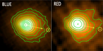
Figure 1: Blue (70 $\mu$m) and Red (160 $\mu$m) 1′$\times$1′ maps of C/2006 W3 (Christensen) observed with PACS on 1 November 2009 UT. Pixel size is 1″ in the Blue map and 2″ in the Red map. Contours levels are stepped by 0.1 in Log, up to 99% of maximum intensity. East is on the left, North is up. The Sun direction is indicated.

2

Figure 2: Spectra of C/2006 W3 (Christensen) obtained with PACS on 8 November, 2009 (central pixel pointed on the comet nucleus). The pixel size is 9.4″$\times$9.4″. The wavelengths of water lines are indicated by vertical dashed lines.

On Nov. 6.59–6.68 UT, the comet was observed using the central pixels on the SPIRE spectrometer for a total duration of 6926 s. The spectral range (450–1550 GHz) encompasses the fundamental ortho 1₁₀–1₀₁ and para 1₁₁–0₀₀ water lines. This source is extremely faint for the SPIRE spectrometer. Standard pipeline reduction shows significant problems with the overall flux level in both the high- (SSW) and low- (SLW) frequency channels. A different approach has been taken therefore that does not rely on the standard pipeline processing. It uses the variation in bolometer temperature to transform the source and dark interferograms into spectra which are then subtracted and divided by a calibration spectrum obtained on a bright source (Uranus). The other aspect that is not currently accurately calibrated in standard processing is the effect of variations in the instrument temperature between the observation of the dark sky and the source: this can cause large relative variations in the recorded spectrum in the low frequency SLW portion. For the data presented here we have determined the overall net flux of the source with no subtraction or addition of flux from the variation in instrument temperature. We then inspect the low frequency spectrum and compare to the spectrum expected from the subtraction of two black bodies at temperatures given by the average instrument temperatures recorded in the housekeeping data. In general, as with the standard pipeline, this gives either too much or too little flux and a non-physical spectrum compared to the spectrum seen in the (unaffected) high frequency band. The difference in model instrument temperatures in the dark sky and the source observation are therefore varied until a match between the overall flux level in SSW is achieved and the flux at the lowest frequencies is zero within the noise. The degree of variation in the temperature difference required to achieve this is less than 1% of the recorded temperatures. The comet is somewhat extended in the beam of the SPIRE spectrometer so a correction is required to the shape of the spectrum to account for the varying beam size of the instrument with frequency (Swinyard et al., 2010). We have normalised this correction here to give the flux in an effective beam size of 18.7″ for both the SSW and SLW channels. Inspection of the data shows that no line is detected within a 3-$\sigma$ upper limit of 0.7–0.8$\times$10^-17 W m^-2. Continuum emission from the coma is detected (Fig. 3).

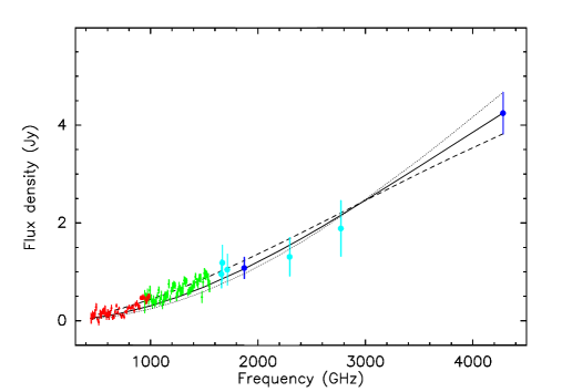
Figure 3: Spectral Energy Distribution of C/2006 W3 (Christensen) combining SPIRE (SLW: red dots; SSW: green dots), PACS photometry (blue dots), and spectroscopy (cyan dots) data, scaled to a Half Power Beam Width of 18.7″ and $\Delta$=3.65 AU. SPIRE data were binned from $\sim$ 0.02 to 0.4 cm^-1. Curves are models for amorphous carbon grains with $a_{max}$= 0.9 mm, and size index –3.6 (solid), –2.8 (dashed), and –3.85 (dotted) (see text).

3 Observations with ground-based telescopes

Table 1: Molecular observations in comet C/2006 W3 (Christensen)

IRAM00UT date	$<r_{h}>$	$<\Delta>$	Line	Intensity	Unit	Velocity shift	Prod. rate
IRAM00[mm/dd.dd]	[AU]	[AU]				[km s-1]	[s-1]
PACS0011/8.74–8.82	3.35	3.70	H2O(212–101)a	$<$ 2.2$\times$10-18a	W m-2	–	$<$ $1.4\times 10^{28}$
SPIRE011/6.59–6.68	3.34	3.65	H2O(111–000)	$<$ 8$\times$10-18	W m-2	–	$<$ $4\times 10^{28}$
Nançay002/10–04/19	3.27	3.90	OH 18 cm	$-0.016\pm 0.003$	Jy km s-1	$-0.32\pm 0.12$	$3.8\pm 0.9\times 10^{28}$
IRAM0009/13.88	3.20	2.57	HCN(1–0)	$-$$0.271\pm 0.015$	K km s-1b	$-0.21\pm 0.03$	$1.6\pm 0.1\times 10^{26}$
IRAM0009/13.93	3.20	2.57	HCN(3–2)	$-$$0.961\pm 0.140$		$-0.15\pm 0.06$	$1.8\pm 0.3\times 10^{26}$
IRAM0009/14.86	3.20	2.59	HCN(1–0)	$-$$0.262\pm 0.013$		$-0.10\pm 0.03$	$1.6\pm 0.1\times 10^{26}$
IRAM0009/14.93	3.20	2.59	HCN(3–2)	$-$$0.972\pm 0.097$		$+0.03\pm 0.04$	$1.6\pm 0.2\times 10^{26}$
IRAM0009/14.88	3.20	2.59	CO(2–1)	$-$$0.433\pm 0.028$		$-0.04\pm 0.03$	$3.9\pm 0.3\times 10^{28}$
IRAM0009/14.40	3.20	2.58	CH3OH($1_{0}$–$1_{-1}$E)c	$-$$0.086\pm 0.011$		$-0.10\pm 0.04$	$1.5\pm 0.3\times 10^{27}$
IRAM0009/14.93	3.20	2.59	H2S($1_{10}$–101)	$-$$0.311\pm 0.031$		$-0.05\pm 0.04$	$1.0\pm 0.1\times 10^{27}$
IRAM0009/14.95	3.20	2.59	CS(2–1)	$-$$0.028\pm 0.012$		–	$0.5\pm 0.2\times 10^{26}$
IRAM0009/14.95	3.20	2.59	H2CO($3_{12}$–$2_{11}$)	$<0.203$		–	$<1\times 10^{27}$
IRAM0010/29.71	3.32	3.48	HCN(1–0)	$-$$0.165\pm 0.010$		$-$$-0.15\pm 0.03$	$1.4\pm 0.1\times 10^{26}$
IRAM0010/29.71	3.32	3.48	CO(2–1)	$-$$0.248\pm 0.026$		$-$$-0.11\pm 0.03$	$3.0\pm 0.3\times 10^{28}$

^a 3-$\sigma$ upper limit per pixel in the central 9.4″$\times$ 9.4″pixel. The upper limit on the flux per beam is estimated to be $\sim$2 times higher. Upper limits for H₂O 2₂₁–1₁₀, 3₁₃–2₀₂, 2₂₁–2₁₂, and 3₀₃–2₁₂ lines are 4.9, 1.8, 1.0, and 3.9 ($\times$10^-18) W m^-2 respectively.

^b For IRAM data, the intensity scale is the main beam brightness temperature.

^c CH₃OH $2_{0}-2_{-1}$E, $3_{0}-3_{-1}$E, $4_{0}-4_{-1}$E, $5_{0}-5_{-1}$E, and $6_{0}-6_{-1}$E lines were also observed with line intensities of $0.083$, $0.062$, $0.049$, $0.043$, and $0.022$ ($\pm 0.010$) K km s^-1, respectively.

Figure 4: Sample of ground-based spectra of comet C/2006 W3 (Christensen): OH spectrum (average of 1665 and 1667 MHz lines) observed at Nançay on Feb. 2 to Apr. 19, and HCN (Sept. 13-14), CO (Oct. 29), and CH₃OH (Oct. 14) spectra observed at the IRAM-30m.

5

Figure 5: Spectra of C/2006 W3 (Christensen) observed with the IRAM 30-m telescope.

6

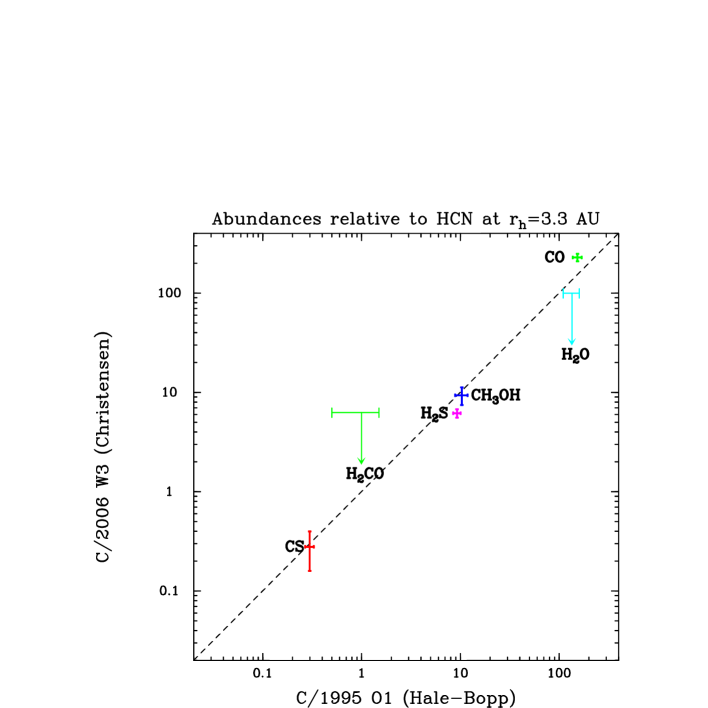
Figure 6: Comparison of measured abundances relative to HCN in comets C/2006 W3 (Christensen) and C/1995 O1 (Hale-Bopp) at 3.3 AU from the Sun.

The OH lines at 18 cm were observed in comet C/2006 W3 (Christensen) with the Nançay radio telescope (Fig. 4, Table 1). The methods of observation and analysis are described in Crovisier et al. (2002). The observations were done pre-perihelion from February 10 to April 19 2009 when the comet was at an average heliocentric distance similar to that of the Herschel post-perihelion observations. An average OH production rate $Q_{\rm OH}$ = $3.8\pm 0.9\times 10^{28}$ s^-1 is derived, which corresponds to a water production rate $Q_{\rm H_{2}O}$ = 1.1 $\times$ $Q_{\rm OH}$ = $4.2\pm 1.0\times 10^{28}$ s^-1, assuming that water is the main source of OH radicals.

Observations with the IRAM 30-m were made on September 12–14 2009 with the recently installed EMIR receiver, completed by a short observation on October 29 just before the Herschel observations (Fig. 4 and $online$ Fig. 5, Table 1). CO, HCN (two rotational transitions), CH₃OH (six lines around 157 GHz) and H₂S were detected. Beam sizes are between 10 and 27″, similar to PACS and SPIRE fields of view.

4 Analysis and discussion

The observed water rotational lines are optically thick (e.g., Biver et al., 2007; Hartogh et al., 2010). To derive upper limits for the water production rate, we use an excitation model which considers radiation trapping, excitation by collisions with neutrals (here CO) and electrons, and solar IR pumping (Biver, 1997; Biver et al., 1999). A H₂O-CO total cross-section for de-excitation of 2 $\times$ 10^-14 cm² is assumed (Biver et al., 1999). The same excitation processes are considered in the models used to analyze the molecular lines observed at the IRAM 30-m. We used a gas kinetic temperature of 18 K, derived from the relative intensities of the CH₃OH lines, and a gas expansion velocity of 0.47 km s^-1, consistent with the widths of lines detected at IRAM. The largest model uncertainty is in the electron density profile. We used the profile derived from the 1P/Halley in situ measurements and scaled it to the heliocentric distance and activity of comet Christensen, as detailed in, e.g., Bensch & Bergin (2004). The electron density was then multiplied by a factor $x_{ne}$ = 0.2, constrained from observations of the 557 GHz water line in other comets (Biver et al., 2007; Hartogh et al., 2010). Upper limits on the water production rate obtained from the 2₁₂–1₀₁ line observed with PACS, and from the 1₁₁–0₀₀ line observed with SPIRE, are given in Table 1. Other observed H₂O lines, either with PACS or with SPIRE, do not improve these limits. The higher water production rate measured pre-perihelion at Nan¸cay may suggest a seasonal effect. As the field of view of the Nan¸cay telescope is large (3.5′$\times$19′), another interpretation is the detection of water sublimating from icy grains. The $Q(\rm H_{2}O)$ measured at Nan¸cay corresponds to a sublimation cross-section of 400 km², or a sublimating sphere of pure ice of 8 km radius.

With a CO production rate of 3$\times$10²⁸ s^-1, comet Christensen is only four times less productive than comet Hale-Bopp at $r_{h}$ = 3.3 AU (Biver et al., 2002). The post-perihelion measurements show that the CO to H₂O production rate ratio in comet Christensen exceeds 220%, indicating a CO-driven activity (Table 1). For comparison, CO/H₂O was $\sim$120% in comet Hale-Bopp at 3.3 AU from the Sun. When normalized to HCN, abundance ratios HCN:CO:CH₃OH:H₂S:CS are 1:240:9:6:0.3 and 1:150:10:9:0.3 for comets Christensen and Hale-Bopp, respectively ($online$ Fig. 6, Biver et al., 2002). Therefore, besides being depleted in H₂O, comet Christensen is enriched in CO relative to HCN, while other molecules have similar abundances.

The dust coma is highly condensed but clearly resolved in both blue (B) and red (R) PACS images (Fig. 1). The width at half maximum of the radial profiles is 9.0″ and 18.1″  in B and R, respectively, a factor 1.64 larger than the PSF ($\sim$5.5″ in B, 11″ in R). The B image is extended Westward towards the Sun direction at PA = 257.5^∘ (phase angle = 16^∘). This asymmetry is also seen in the R image. HCN and CO spectral lines are similarly blue-shifted (Table 1), which indicates preferentially dayside emission of these molecules from the nucleus, and is consistent with the dust coma morphology. Since CO is likely the main escaping gas (CO₂ has been observed to be less abundant than CO in comets Bockelée-Morvan et al., 2004), dust-loading by CO gas is suggested. The enhanced CO production towards the Sun implies sub-surface production at depths not exceeding the thermal skin depth ($\leq$ 1 cm). The distant CO production in comet Christensen may result from the crystallization of amorphous water ice immediately below the surface (Prialnik et al., 2004).

Radial profiles in the B and R bands are presented in Fig. 7 for both the comet and the PSF (from Vesta data). Although highly structured, the background has been estimated as best as possible and subtracted. The PSF has a complex shape which has been fitted radially with two gaussian profiles centered at $\rho$ = 0 and $\rho$ = 6″ (resp. 12″) for the B (resp. R) bands. A symmetric 2D PSF has then been constructed and convolved with theoretical cometary surface brightness profiles $S_{B}\propto\rho^{-x}$. One finds that the full range of radial profiles can be reproduced with $0.8<x<1.2$. Most of the dispersion is likely due to the PSF structure and more specifically to its extended tri-lobe pattern (Lutz, 2010). The average surface brightness profiles can be fitted with $x=1.05\pm 0.05$ in the B band and $x=1.00\pm 0.05$ in the R band. The radial dependence of the surface brightness is then compatible with the steady-state $\rho^{-1}$ law in the full 60–210 $\mu$m spectral range.

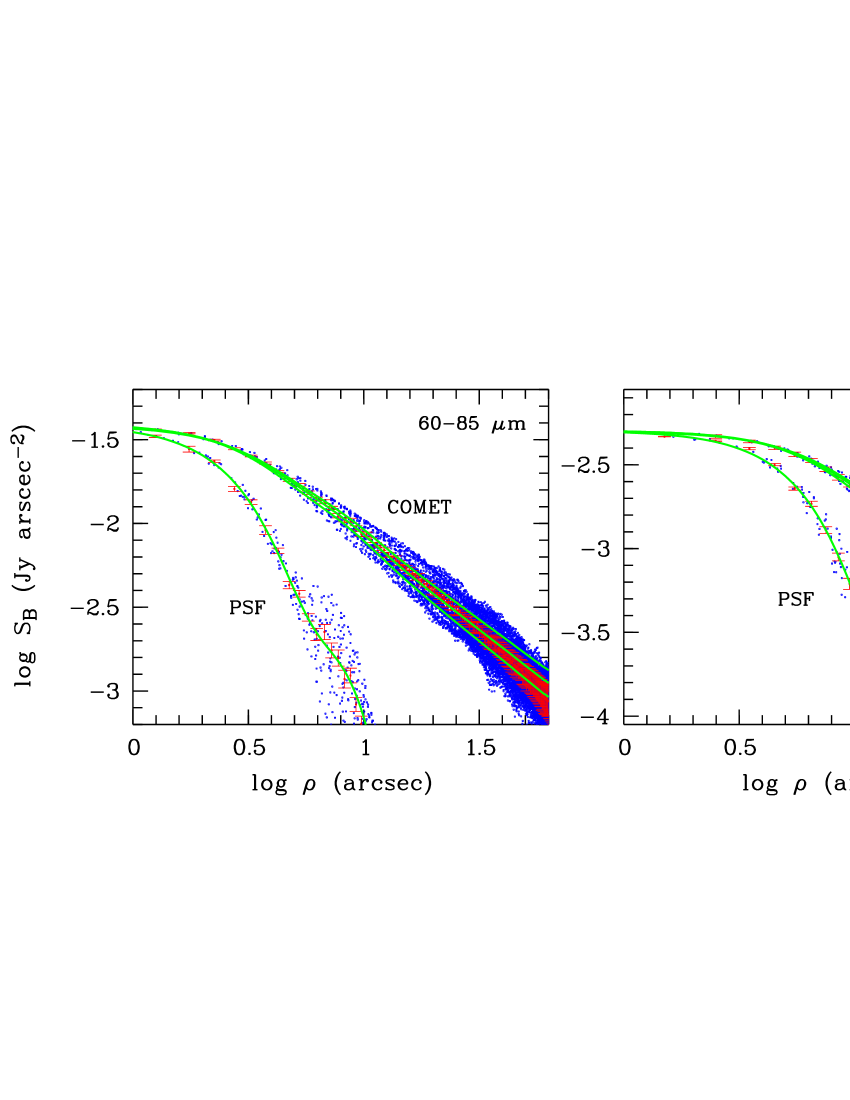
Figure 7: Comet surface brightness and re-scaled PSF (Vesta) in B (left box) and R (right box) bands. Blue dots: surface brightness for each pixel. Red dots: mean values in 0.5″ (B) or 1.0″ (R) wide annuli, with error bars. For the comet, the continuous green lines are radial profiles obtained by convolving a $\rho^{-x}$ law with the PSF with, from top to bottom, x = 1.0, 1.05, 1.1 (B) and x = 0.95, 1.0, 1.05 (R). The green line superimposed on Vesta data is the PSF model (see text).

There is then no evidence for a significant contribution of nucleus thermal emission in the central pixels. Assuming that the CO production rate scales proportionally to the nucleus surface area, the size of Christensen’s nucleus is estimated to be a factor of two smaller than Hale-Bopp’s nucleus size, i.e. $D$$\sim$ 20 km for comet Christensen (see Altenhoff et al., 1999, for Hale-Bopp’s nucleus size). From the Standard Thermal Model (Lebofsky & Spencer, 1989) with the nucleus albedo set to 4% and the emissivity and beaming factor taken as unity, a 20 km diameter body would contribute to 4.5% of the flux measured in the central 1″ pixel of the B image ($F_{\rm B}$ = 38.4 mJy/pixel), and still less (2%) in the R image where the measured peak intensity is $F_{\rm R}$ = 19.5 mJy/pixel (2″-pixel). From the B image, we estimated that $D<26$ km.

The Spectral Energy Distribution (SED) of the dust thermal emission can constrain important properties of cometary dust, in particular the dust size distribution and production rate (Jewitt & Luu, 1990). The flux density in the SPIRE spectrum (Fig. 3) varies as $\nu^{-1.78}$. The spectral index, close to $\alpha$ = 2, indicates the presence of large grains, consistent with the maximum ejectable dust size loaded by the CO gas ($a_{max}$ $\sim$ 0.9 mm for a $D$ = 20 km body of density $\rho_{N}$ = 500 kg m^-3, with the dust density $\rho_{d}$ = $\rho_{N}$; $a_{max}\propto D^{-3}$; Crifo et al., 2005). We modelled the thermal emission of the dust coma following Jewitt & Luu (1990). Absorption cross-sections calculated with the Mie theory were used to compute both the temperature of the grains, solving the equation of radiative equilibrium, and their thermal emission. Complex refractive indices of amorphous carbon and olivine (Mg:Fe = 50:50) (Edoh, 1983; Dorschner et al., 1995) were taken as broadly representative of cometary dust. We considered a differential dust production $Q_{d}$(a) as a function of size, with sizes between 0.1 $\mu$m and 0.9 mm. The size-dependent grain velocities $v_{d}$(a) were computed following Crifo & Rodionov (1997) assuming $D$ = 20 km, and vary from 6 to 224 m s^-1 ($\propto$ $a^{-0.5}$ at large sizes). We assumed a local dust density $\propto r^{-2}$, where $r$ is the distance to the nucleus, consistent with the maps. The best fit to the flux ratio $F_{\rm B}/F_{\rm R}$ in R and B bands is obtained for $Q_{d}$(a) $\propto$ $a^{-(3.6^{+0.25}_{-0.8})}$, which yields a dust opacity (the ratio between the effective emitting dust cross-section and dust mass), of 6.8${}^{+1.2}_{-2.8}$ and 5.7${}^{+0.3}_{-1.3}$ m² kg^-1 at 450 GHz, and dust production rates of 850${}^{+1100}_{-200}$ and 920${}^{+730}_{-110}$ kg s^-1, for carbon and olivine grains, respectively. The whole SED between 450 and 4300 GHz is consistently explained (Fig. 3). Assuming that CO is the main gas escaping from the nucleus, the inferred dust to gas mass production ratio is then 0.5 to 1.4.

5 Conclusions

Comet Christensen was a distant comet. Nevertheless, the continuum was clearly detected by PACS and SPIRE, providing useful constraints on the properties of the cometary dust. Although water emission was not detected in this object, the limits obtained are significant. The prospects for future cometary studies with Herschel are thus very good.