The VLA-COSMOS Survey. IV. Deep Data and Joint Catalog

Abstract

In the context of the VLA-COSMOS Deep project additional VLA A array observations at 1.4 GHz were obtained for the central degree of the COSMOS field and combined with the existing data from the VLA-COSMOS Large project. A newly constructed Deep mosaic with a resolution of 2.5^′′ was used to search for sources down to 4$\sigma$ with 1$\sigma\approx 12\,\mu$Jy/beam in the central 50${}^{\prime}\times$50^′. This new catalog is combined with the catalog from the Large project (obtained at 1.5^′′$\times$1.4^′′ resolution) to construct a new Joint catalog. All sources listed in the new Joint catalog have peak flux densities of $\geq$5$\sigma$ at 1.5^′′ and/or 2.5^′′ resolution to account for the fact that a significant fraction of sources at these low flux levels are expected to be slighty resolved at 1.5^′′ resolution. All properties listed in the Joint catalog such as peak flux density, integrated flux density and source size are determined in the 2.5^′′ resolution Deep image. In addition, the Joint catalog contains 43 newly identified multi-component sources.

1. Introduction

In recent years, several cosmological deep fields have been imaged at 20 cm (e.g., Richards, 2000; Bondi et al., 2003; Condon et al., 2003; Hopkins et al., 2003; Seymour et al., 2004; Norris et al., 2005; Huynh et al., 2005; Fomalont et al., 2006; Simpson et al., 2006; Ivison et al., 2007; Schinnerer et al., 2007; Miller et al., 2008; Owen & Morrison, 2008) providing a few thousand radio sources down to flux limits of a few 10 $\mu$Jy. These deep radio imaging data are sensitive enough to detect star forming galaxies with star formation rates of several 10 to 100 $\>{\rm M_{\odot}yr^{-1}}$ out to and beyond a redshift of $z$ $\sim$ 1. Similarly, radio galaxies can be seen out to redshifts of $z$ $\sim$ 5 and the most luminous ones even well into the epoch of reionization. Thus, deep radio images in conjunction with deep imaging data at X-ray, optical and infrared wavelengths are ideal to investigate the dust-unbiased star formation, the evolution of radio(-loud) AGN, as well as the population mix of radio sources in the first place.

In order to study the cosmological evolution of galaxies and black holes, it is not only important to overcome the effect of cosmic variance (e.g. by studying a large enough area) but also to understand the effect of large scale structure on the evolution (e.g. by covering a large contiguous area). To address the second effect in particular, the Cosmic Evolution Survey (COSMOS) collaboration has conducted panchromatic imaging and spectroscopy of an equatorial field with a size of 2 $\rm deg^{2}$ (for an overview, see Scoville et al., 2007b) ranging from X-ray XMM-Newton and Chandra (Hasinger et al., 2007; Elvis et al., 2009), UV GALEX (Zamojski et al., 2007), optical and near-infrared ground-based (Taniguchi et al., 2007; Capak et al., 2007), optical HST (Scoville et al., 2007a; Koekemoer et al., 2007), mid- to far-infrared Spitzer (Sanders et al., 2007), millimeter (Bertoldi et al., 2007; Scott et al., 2008) and radio VLA (Schinnerer et al., 2004, 2007) imaging to extensive optical spectroscopy using the VLT/VIMOS and Magellan/IMACS instruments (Lilly et al., 2007; Trump et al., 2007). Most of these datasets are now publicly available from the COSMOS archive at IPAC/IRSA.

The VLA-COSMOS survey at 20 cm is part of the overall imaging effort and its scientific goals and motivation have been described in detail by Schinnerer et al. (2007). Initial observations from a pilot project testing the mosaicking strategy and giving a first source catalog are presented by Schinnerer et al. (2004). As a large NRAO/VLA program, the VLA was used in A and C configuration to cover the entire COSMOS field resulting in an image with uniform noise properties in the central 1$\times$1 deg² and an average rms of 10.5 $\mu$Jy. Schinnerer et al. (2007) provide a detailed description of the survey set-up, the data reduction, as well as the testing and construction of the final VLA-COSMOS Large project catalog (hereafter: Large catalog). Subsequently, Bondi et al. (2008) derived the completeness of the Large catalog and also analyzed the effect of bandwidth smearing on the derived source flux densities to obtain the source counts. Although the VLA-COSMOS Large Project dataset has been used for several scientific results on, e.g. the faint radio population, the radio-derived star formation rate density, the radio AGN population and stacking of high-z galaxy populations (Smolčić et al., 2008, 2009a, 2009b; Carilli et al., 2007, 2008), the need for deeper radio imaging data became apparent during the search for radio counterparts to millimeter sources from the COSMOS MAMBO mapping data (Bertoldi et al., 2007); the Large project only provided counterparts for about half of the mm-sources. Thus, the Deep project was initiated with the aim of doubling the integration time for the central seven pointings which fully cover the MAMBO 1.2 mm map of the COSMOS field. These new observations are described here.

The paper is organized as follows: After a description of the new observations and the data reduction (§2), the revision of the Large catalog (leading to a new version of v2.0) and the construction of the new Deep catalog are outlined in §3 and §4. In §5 we explain the construction of the final Joint catalog which is described in detail in §6 where we also present all the tests and corrections involved. A summary is given in §7.

2. Observations and data reduction

The central seven pointings of the mosaic for the VLA-COSMOS Large project (pointing numbers: F07, F08, F11, F12, F13, F16, F17; see Schinnerer et al., 2007) were observed using the VLA A configuration in February and March 2006. The observations were executed on 11 days, typically lasting for a total of six hours starting at 07hr LST (Local Sidereal Time). The exact coordinates of the pointing centers are listed in Tab. 1. We used the same spectral set-up and set of calibrators as for the VLA-COSMOS Large project to allow for an easy combination of the data from the two projects: the VLA standard L-band continuum frequencies of 1.3649 and 1.4351 GHz in multi-channel continuum mode, the quasar 0521+166 (3C 138) for flux and bandpass calibration at the beginning of each day, and the quasar 1024-008 as phase calibrator. In order to obtain a good sampling of the uv-plane, we cycled three times through the pointings each day with a total integration time per pointing of $\sim$45 min. The final resulting integration time per pointing was $\sim$8.25 hr. In addition, we changed the order of the observations of the individual pointings each day to sample the uv plane uniformly in all pointings.

During the data reduction process, we excluded all EVLA antennas that were present in the array during the observations. We followed the data reduction procedure adopted for the Large project (Schinnerer et al., 2007) which uses the Astronomical Imaging Processing System (AIPS; Greisen, 2003). uv data points affected by RFI (radio frequency interference) were again flagged by hand using the task TVFLAG and by excluding amplitudes greater than 0.55 Jy. The flux density of the phase calibrator 1024-008 was found to be close to its previous value in the season of 2004/5. After final calibration, the Deep data were combined with the uv data of the corresponding pointings from the Large project.

The final imaging was performed using the task IMAGR with the same settings as for the Large project, i.e. the same tiling of the individual pointings and the associated CLEAN boxes were used, the flux cut-off was kept at 45 $\mu$Jy, and the restoring beam was again set to 1.5${}^{\prime\prime}\times$1.4^′′. The robust parameter was changed from 0 to 0.25 to obtain a dirty beam as close as possible to the final CLEAN beam. As for the Large project, each polarization for each intermediate frequency (IF) was CLEANed separately and combined afterwards in the image plane. The final seven new fields were combined with the existing 16 fields from the Large project to obtain a mosaic covering the full 2 deg² of the COSMOS field. The average rms achieved in the central 30^′ was 8 $\mu$Jy/beam at the resolution of the Large project. In order to mitigate the effect of bandwidth smearing on the derived peak flux densities during source extraction (see §6.1), the final mosaic was convolved to a lower resolution of 2.5^′′ (Fig. 1) leading to an increase of the rms to $\sim$12 $\mu$Jy/beam. We tested several convolution kernels by comparing the source fluxes and the number of sources extracted for two representative sub-images of the mosaic. The resolution of 2.5^′′ provided the best compromise between minimizing the flux losses and maximizing the number of extractable sources. We verified that the noise distribution in the Deep image follows a Gaussian distribution as expected (Fig. 2). This Deep mosaic was used for source detection and extraction (see §4). Fig. 3 shows the fractional area covered as a function of rms for the Deep and Large mosaics.

3. The Revised Large Project Catalog

The original source catalog for the VLA-COSMOS Large Project presented by Schinnerer et al. (2007) was created by the following procedure: 1) the AIPS task SAD extracted candidate components down to a peak flux density limit of 3$\sigma$, 2) after fits to the peaks of these candidates using MAXFIT only those with an measured (rather than the fitted Gaussian) peak flux density of $\geq$4.5$\sigma$ were kept, 3) components potentially missed by SAD were recovered with JMFIT which was used to fit a Gaussian to all peaks above our detection threshold that were not included in the SAD component list, and finally 4) components not in the SAD list but with non-zero major axes found in step 3 were added. This component catalog was transformed into a source catalog, after multi-component sources, e.g. large radio galaxies, were identified by visual inspection. Since in the case of faint sources, the position and peak values of a Gaussian parametric fit might not be a good representation of the real values, the position and value of the peak found by MAXFIT replaced the results from the Gaussian fit. Furthermore, all sources classified as unresolved (for our methodology see Section 6.2 in Schinnerer et al., 2007) had their integrated flux density set equal to the peak flux density. The final VLA-COSMOS Large project catalog (v1.0) has a total of 3601 entries.

Subsequent use of the Large catalog in conjunction with the COSMOS optical and (near- to mid-)IR catalogs and images showed that the fraction of spurious sources increases significantly below 5$\sigma$. Spurious sources in our definition are sources that lie in a noisier environment than expected for a $>4.5\sigma$ detection, i.e. three or more 3$\sigma$ peaks are present in a 10${}^{\prime\prime}\times$10^′′ box centered on the source. The misidentification is likely due to a mismatch in the derived rms value (in a 17.5${}^{\prime\prime}\times$17.5^′′ box) and the local rms distribution at the exact position of the source. This finding is also confirmed by a comparison of sources present in the Large and Deep catalogs (see §5.2.1). Thus we exclude all sources below 5$\sigma$ from the revised Large catalog. In addition, the correction for bandwidth smearing as derived by Bondi et al. (2008) has been applied to the peak flux densities and the classification into resolved and unresolved sources has been modified accordingly (for details see Bondi et al., 2008). The revised version of the VLA-COSMOS Large project catalog [hereafter: Large catalog (v2.0)] contains a new total of 2417 sources. The revised VLA-COSMOS Large project catalog (v2.0) has been publicly released to the COSMOS archive at IPAC/IRSA.

4. Identification of Deep Project Sources

As the rms is less uniform in the Deep mosaic than in the Large mosaic and shows a steep increase towards the edges, applying a simple flux density cut for source detection is not possible. In order to use the AIPS source/component finding task SAD, a $S/N$ map was created. First, a sensitivity map (Fig. 4) was constructed using the AIPS task RMSD with a box size of 105${}^{\prime\prime}\times$105^′′ to estimate the rms and a sampling step size of 2.45^′′ in both RA and DEC. To obtain the final input $S/N$ map for SAD, the Deep image was divided by the sensitivity map and blanked at the edges where the rms values in the sensitivity map exceeded 34 $\mu$Jy/beam (the largest rms value present in the Large mosaic). This last step allowed us to search for sources in the corners/edges of the mosaic, whereas the area corresponding to the COSMOS field was searched for the construction of the Large catalog (see Schinnerer et al., 2007).

SAD was set to search for sources in six iterations with cut-off levels for the peak of 10, 8, 7, 6, 5, and 4$\sigma$. The derived values in units of $S/N$ were converted to mJy/beam using the corresponding rms values from the sensitivity map. As in the case of the Large project sources with complex structures – e.g. radio galaxies – were fitted by multiple Gaussian components, such that the derived catalog contains components rather than real sources. In order to identify these multi-component sources, we compared by eye the location of the multi-component sources from the Large catalog (v2.0) with the component list obtained for the Deep image to identify the components belonging to the same source. During the comparison with the Large catalog (v2.0), it was noticed that several slightly extended sources were fitted by two separate components with a typical separation of $\sim$1^′′ (hereafter: ‘twin’ sources). In order to determine the nature (simple extended Gaussian vs. truly non-Gaussian geometry) of these ’twin’ sources, a single Gauss component was fitted to these sources using JMFIT. If the integrated flux density of this single Gaussian fit was consistent within the formal errors with the combined integrated flux densities of the two components derived by SAD, we replaced the ‘twin’ sources by a single object.

5. Construction of the Joint Source List

Based on the size distribution of faint radio sources (e.g. Muxlow et al., 2005; Fomalont et al., 2006; Owen & Morrison, 2008; Bondi et al., 2008) a significant fraction of sources should be resolved at our flux limit and resolution. Owen & Morrison (2008) showed that source extraction at different resolutions is ideal to maximize the number of sources found. Therefore, the combination of the VLA-COSMOS Large and Deep catalogs is ideal to find a maximum number of sources for inclusion in a joint catalog. In the following we describe the steps taken to identify such radio sources in the VLA-COSMOS mosaics.

In order to construct a list of radio sources from the two separate catalogs, we used the following process that is described in detail below: First, sources present in both catalogs were included (§5.2), then selected sources detected only in the Large Project mosaic were added (§5.3.1), as were – finally – a number of sources present only in the Deep catalog (§5.3.2). In order to minimize the inclusion of spurious sources at the low significance end, the local rms was re-examined at 1.5^′′ and 2.5^′′ resolution. All sources having a final peak $S/N\geq 5$ at at least one resolution were included.

An overview of the number of sources selected from the Large (v2.0) and Deep catalog for inclusion in the Joint catalog is given in Tab. 2, together with a listing of some key properties.

5.1. Estimate of the Local Background Noise

Based on the experience with the Large catalog (v1.0) it is important to obtain an accurate estimate of the local rms to properly measure the $S/N$ of individual radio sources. In order to find the optimal box size for the local rms estimate, we compared the value in the rms map used for source detection (see §4) to that obtained if a smaller box is used. We chose a box size of 50 pixel (=17.5^′′) to obtain a good estimate of the rms around compact sources. Fig. 5 shows the different rms values obtained with a 105^′′ and 17.5^′′ box for a number of low $S/N$ sources from the deep catalog and highlights the importance of deriving an accurate local rms estimate. The choice was based on the finding that a box size of 17.5^′′ used for the Large catalog still resulted in a number of spurious sources at the low $S/N$ end and the requirement that at 2.5^′′ resolution the number of pixels outside the source should still be sufficient.

We constructed new rms maps at 1.5^′′ and 2.5^′′ resolution using a box size of 50 pixels with the task RMSD and subsequently used them to estimate the local rms. We refer to this revised $S/N$ as the ‘local’ $S/N$ ($S/N_{17.5^{\prime\prime}}$). All sources with a $S/N_{17.5^{\prime\prime}}\geq 5$ will be included in the joint source list.

5.2. Sources Present in Both Catalogs

For many sources in the Deep catalog it was possible to identify counterparts in the Large catalog (Schinnerer et al., 2007) down to 5$\sigma$ or even 4.5$\sigma$. The successfully matched sources include all but one of the objects already known from the Large Project to consist of multiple Gaussian components and the majority ($\sim$60%) of the single component sources in the Large catalog (v1.0).

5.2.1 Identification of Single-Component Sources

To identify radio sources present in both the Deep and Large catalog, we used the Large catalog down to 4.5$\sigma$. We matched the two catalogs with a search radius of 1.5^′′ to account for offsets between the peak positions for extended objects. The spatial characteristics of the noise in the Deep and Large image differ due the additional coverage of the central seven pointings by the Deep project and due to the differences in the final resolution (2.5^′′ in the Deep mosaic vs. $\sim$1.5^′′ in the Large mosaic; see §2).

As mentioned in Section 3 the occurrence of spurious sources in the Large catalog is significantly reduced by omitting sources in the range $S/N_{\rm Large}\in$ [4.5, 5[. The added depth gained with the Deep project observations in the central 40^′ (Fig. 6) should increase the reliability of sources with $S/N_{\rm Large}<$ 5 in the Large Project catalog (v1.0) within this area. Fig. 6 shows the corresponding detection thresholds of the two images. The peak flux densities of sources in the Large catalog (v1.0) are plotted as a function of their radial distance from the field center, their lower envelope roughly tracing the average $S/N$ detection threshold of 4.5$\sigma$ (used as cut for the Large catalog (v1.0)). The radial evolution of the mean rms (${\rm\overline{rms}}$) was calculated in concentric rings with a width of 2^′ using the respective sensitivity maps for both images (Fig. 4 for the Deep mosaic and Fig. 12 in Schinnerer et al. (2007) for the Large one). The ‘bump’ in the measured mean noise level at a radius $r\approx$ 45^′ is due to the sensitivity maps’ rectangular geometry. In order to obtain an estimate of the minimal average noise level at this distance from the field centre we fitted a cubic spline to the measured ${\rm\overline{rms}}$ in this region. The resulting curve for the Large mosaic, when scaled to 4.5$\sigma$, defines a lower envelope to the measurements (ignoring detections in sites with locally lower rms noise). The 4$\sigma$ limit of the Deep catalog corresponds to the 4.5$\sigma$ limit of the Large catalog for the inner radii with $r\leq 15^{\prime}$ while it increases to the 5$\sigma$ limit of the Large catalog at larger radial distances.

The fraction of sources in the VLA-COSMOS Large catalog (v1.0) which are at a given distance from the field centre and have $S_{\rm peak}<4\sigma_{\rm Deep}$ is shown in Fig. 6b. The increase of this fraction with distance from the field center will affect the radial dependence of the number of successful matches between the two catalogs. We verified that the success rate of the catalog matching shows no distance dependence (Fig. 7). While the fraction of sources in the Large catalog (v1.0) for which a counterpart could be identified decreases at larger distances (solid black line), the effective matching success rate defined as ratio of the measured matching success rate and the fraction of sources with peak flux densities below 4$\sigma$ in the Deep mosaic stays basically constant (thick grey line) within a range of 60 and 80%.

Thus we conclude that the direct positional correlation of catalog entries has not caused sources to be systematically missed as a function of (radial) field distance in the VLA-COSMOS Deep mosaic.

Before final inclusion in the source list we checked for each of the successfully matched sources that it met our selection criterion of peak $S/N_{17.5^{\prime\prime}}\geq 5$ at either 1.5^′′ or 2.5^′′ resolution in the deep data. If this requirement was not satisfied the corresponding source was not considered any further.

5.2.2 Identification of New Multi-Component Sources

As already stated above, all but one of the multi-component sources listed in the Large catalog (v2.0) were also present in the Deep catalog. However, during the merging of the two catalogs 43 new multi-component sources were identified. Image cutouts of all new multi-component sources are shown in Fig. 8.

During the cross-correlation of the Large and Deep catalog several sources were recognized to constitute sources made up of several (Deep) rather than just a single (Large) Gaussian component during visual inspection of all sources. In addition to this, several Deep sources found in the neighborhood of multi-component objects (identified in the Large catalog) were subsequently assigned to these sources as additional components of their extended emission. In one instance two of the former multiple component sources were joined to form a new, larger multiple component source (a bipolar jet with nucleus assigned the new Joint catalog ID COSMOSVLADP_J095758.04+015825.2: - the three merged components have the following IDs in the VLA-COSMOS Large Project catalogs: COSMOSVLA_J095755.84+015804.2, J095758.04+015825.2 & J095800.79+015857.1). Besides these newly identified or augmented multi-component sources there was also a small number of multi-component sources that had either (i) not been previously listed in the Large catalog or (ii) are situated outside the area searched during the construction of the Large catalog.

5.3. Sources present in only one catalog

Apart from the sources that are present in both catalogs, objects present only in one of the two catalogs have been added to the list as well. The exact procedures adopted are described in the following.

5.3.1 Sources identified in the Large image only

All sources in the Large catalog (v2.0) with a $S/N_{\rm Large}\geq 5$ but without a match in the Deep catalog are in principle valid candidates for inclusion in the joint source list, provided they are not flagged as detections potentially due to side lobes of strong radio sources. Since SAD tries to fit Gaussians to all peaks above a certain limit, the fact that certain sources were not found by SAD during the construction of the Deep catalog suggests that some of these objects might be mere noise peaks or have very unusual morphologies. Similarly, we expect that a fraction of the sources with $S/N<4.5$ might be real.

Therefore, we measured for all sources in the Large catalog (v1.0) without a match in the Deep catalog the peak flux density in the Deep image at 1.5^′′ and 2.5^′′ resolution at the according position from the Large catalog following the steps described in §6.2.1 and subsequently discarded 959 candidates with $S/N_{17.5^{\prime\prime}}<5$ at both resolutions while it was possible to keep 393 of the unmatched sources with $S/N_{\rm Large}\geq 4.5$ from the Large catalog (v1.0).

5.3.2 Sources identified in the Deep image only

1155 objects – predominantly in the range of 4$\leq S/N_{\rm Deep}<$8 – were detected in the Deep mosaic which did not have a counterpart in the original Large catalog (v1.0). In order to assess the significance of these sources which are potentially new detections due to the different source extraction area for the Deep catalog, the increased sensitivity in the central square degree and the fact that the larger beam is more sensitive to slightly extended sources (as SAD works with peak fluxes), we adopted the approach outlined below. While the $S/N_{\rm Deep}=$ 4 cut corresponds at least to the detection threshold used for the original Large catalog, our experience with this catalog showed that the number of spurious sources rises significantly below $S/N<$ 5 due to small mismatches between the real local rms and the estimated value in the constructed rms map.

Thus, the local $S/N$ was checked at 2.5^′′ resolution as well as at 1.5^′′ resolution. All sources with $S/N_{17.5^{\prime\prime}}\geq$ 5 were included in the joint list. In total, 178 of 283 unmatched Deep detections with $S/N_{\rm Deep}\geq$ 5 were taken over in the Joint catalog. Of 872 sources with 4 $\leq S/N_{\rm Deep}<$ 5 some 136 met our selection criteria.

6. Joint Catalog

In the following we describe how the flux densities and all other measurements provided in the catalog were derived and which corrections have been applied to the tabulated values.

6.1. Correction for Bandwidth Smearing

Bandwidth smearing (BWS) can occur in radio synthesis imaging when a finite frequency range is observed. It causes a radial smearing that becomes more severe with increasing distance from the phase center (or center of a pointing), as the phase calibration is mathematically speaking only correct for a given frequency at the phase center. Thus the effect is similar to chromatic aberration in optical imaging. A detailed explanation and discussion of the effect of bandwidth smearing for the VLA is given, e.g., by Thompson (1999) and Bridle & Schwab (1999).

For the VLA-COSMOS project with an observed bandwidth of 3.125 MHz for a single channel, a (final) radial smearing of 2.25^′′ is expected at a radial distance of 15^′ from the pointing center, i.e. close to the cut-off radius of the individual pointings used when creating the mosaic (for equations and details, see Bridle & Schwab, 1999). This bandwidth smearing effect also causes a decrease of the peak flux density as the emission is now distributed over a larger area. The integrated flux density, however, will not be affected. As sources in the final mosaic can be covered by up to 7 individual pointings, the impact of bandwidth smearing strongly varies at each location in the mosaic as a given source is separated by a different amount from the centers of the individual pointings.

Thus, the effect of bandwidth smearing depends on the resolution of the image. In correcting the measurements presented in the Large catalog (v2.0) for the BWS effect Bondi et al. (2008) adopted the approach of boosting the measured values of the peak flux density $S_{\rm peak}$ by different amounts depending on the distance from the center of the VLA-COSMOS field. The boost factors were derived from tests comparing the peak flux densities of sources at the centers in individual pointings and the derived flux densities in the final Large mosaic. This approach can be used because the sensitivity map (cf. Fig. 12 in Schinnerer et al. (2007)) for the VLA-COSMOS Large project is fairly uniform over significant areas, i.e. all locations suffer similarly from the combined BWS effect of the contributing pointings. However, the additional data for the central seven pointings for the Deep Project changed the uniformity of the sensitivity distribution over the COSMOS field. We thus examine both the method of Bondi et al. (2008) as well as an alternative based on a modeled sensitivity map for the VLA-COSMOS Deep project.

The model sensitivity distribution for an individual pointing was constructed using the beam pattern for a VLA antenna at 1.465 GHz, as specified in the help page for the AIPS task PBCOR:

$$1-1.343\times 10^{-3}~{}\mathscr{X}^{2}+6.579\times 10^{-7}~{}\mathscr{X}^{4}-1.186\times 10^{-10}~{}\mathscr{X}^{6}~{},$$ (2)

where $\mathscr{X}$ is the product of the distance from the pointing center in arcminutes with the observing frequency in GHz. The full model sensitivity map (Fig. 11) was then assembled by adding the individual beam patterns which were weighted according to the observation time dedicated to each pointing (i.e., the central 7 pointings were weighted more strongly than the others by a factor of 1.4).

To estimate the magnitude of the required BWS correction we closely follow the procedure described by Bondi et al. (2008). In brief, a primary beam correction was applied to the images of the 23 individual pointings and they were convolved to the same resolution of FWHM 2.5^′′ as the Deep mosaic. Then we measured the peak flux densities of selected sources in these individual images and compared their values with those obtained from the same measurement carried out at the corresponding position in the mosaic.

At this stage, it is mandatory to use sources with a peak flux density that has not been significantly diminished by the BWS effect. The dimensionless parameter $\beta=\frac{\Delta\nu}{\nu_{0}}\frac{\theta_{0}}{\theta_{\rm FWHM}}$ (see Bridle & Schwab (1999) and the VLA observational status summary) makes it possible to infer the amount by which peak flux densities are reduced. In the case of the VLA-COSMOS Large image with an adopted beam width of $\theta_{\rm FWHM}\sim$ 1.5^′′ the peak flux densities of sources within 5^′ of the pointing centers are expected to be reduced by less than 5%. At a resolution of $\theta_{\rm FWHM}\sim$ 2.5^′′, as in the case of the Deep image, the same small decrease still exists as far as 8^′ from the pointing center. Thus we were able to use a contiguous area covering a significant fraction of the entire VLA-COSMOS mosaic (see area indicated by dashed white circles in Fig. 11). A correspondingly larger number of sources could thus be used to check the validity of the adopted method for BWS correction. In the following we will quantify the magnitude of the BWS effect using only sources within 5^′ of the center of either of the 23 VLA-COSMOS pointings – this ensures that peak flux densities measured on individual pointings should differ by less than 2% from the nominal value – and we will use the larger number of sources out to 8^′ to check the quality of the approach. Since the aim is to correct for the BWS effect introduced by overlapping pointings, strictly speaking no (valid) corrections can be derived for sources located in the edges (i.e. those covered by only single pointing, see Fig. 12).

Fig. 12 shows the comparison of the two different methods to correct for the BWS effect. It should be noted that the maximum decrease observed is only 10%. The top row displays the uncorrected values of the quantity $\mathscr{S}=S_{\rm peak,~{}mosaic}/S_{\rm peak,~{}pointing}$, i.e. the ratio of the peak flux densities measured in the mosaic and in an individual pointing, as a function of normalized sensitivity (left column) and radial distance from the field center (right column). The median ratio $\langle\mathscr{S}\rangle$ of peak flux densities in a specific bin is marked by an open circle. The associated error bars span the interquartile range of $\mathscr{S}$ within a bin in distance or model sensitivity. Median and errors are reported in red when only sources within 5^′ of the center of one of the 23 pointings are used (i.e. only the red points) and in black when all sources within 8^′ are considered (i.e. the red and grey points).

It is obvious from the upper row of Fig. 12 that the effect of bandwidth smearing disappears (i.e. the value of the ratio $\mathscr{S}$ approaches unity) towards the edge of the field where there are no overlapping pointings or, conversely, at lower sensitivity values which stem from regions in the field covered by only one pointing. The best-fitting linear trends define which BWS correction should be applied to sources lying at a given distance or within a region of a specific sensitivity value, depending on the method considered. In the middle row the ratios $\mathscr{S}_{\rm sensitivity~{}correction}$ are corrected according to the second method using the model sensitivity map (Fig. 11), i.e. the the slope of the line as a function of sensitivity (upper left panel). Thus the distribution of $\mathscr{S}$ is necessarily flat when plotted as a function of model sensitivity. This flatness is also preserved when the corrected peak flux densities are plotted against distance from the center of the field. The BWS correction (third row) based on the comparison of the peak flux density ratios as a function of distance from the center of the VLA-COSMOS field following Bondi et al. (2008) also fares well in straightening the distribution of corrected ratios $\mathscr{S}_{\rm distance~{}correction}$ with respect to both distance (again, a requirement) and model sensitivity. However, a weak correlation of peak flux density ratios with sensitivity is still present after the application of this method. Therefore we conclude that the sensitivity-based approach is slightly better for BWS correction and will use it to compute the corrected peak flux density, $S_{\rm peak,\,corr.}$, provided in the Joint catalog (see also Tab. 3).

6.2. Catalog Entries

6.2.1 Single-component sources

95% of the sources in the VLA-COSMOS Joint catalog are well fit by a single Gaussian component. The following five steps were required to obtain the position, peak and integrated flux density, as well as the size for each source. All measurements described in the following were carried out on the Deep Mosaic. In particular, this also applies to those sources which were not part of the initial Deep catalog (see §5.3.1).

1. The (parametric) integrated flux $S_{\rm total}$ was derived using the task SAD. In the case of the ‘twin’ sources, JMFIT was used instead (for details see §4). At the same time the convolved shape parameters were determined.

2. The peak flux density was obtained using the task MAXFIT. The square search box for MAXFIT was centered on the position of the Gaussian fit from the previous step. We used an initial box size of 3 pixels that was increased in steps of 2 pixels if MAXFIT did not converge. The measured peak flux density $S_{\rm peak}$ was corrected for the effects of bandwidth smearing (see §6.1) resulting in the corrected measured peak flux density $S_{\rm peak,\,corr.}$.

3. The source position was set to the position of the MAXFIT peak.

4. As a significant fraction of sources is resolved at the faint flux levels probed here, it is necessary to classify the sources into resolved and unresolved. We followed the approach used by Schinnerer et al. (2007) and Bondi et al. (2008). The method relies on the fact that the ratio between integrated and peak flux density is a measure of the spatial extent of a radio source. A detailed description of the method is given in Appendix A together with a description of a suite of Monte Carlo simulations which we use to calibrate our classification scheme. Fig. 13 is the diagnostic diagram used to identify the resolved sources based on our simulations. The line defining the lower boundary to the locus of resolved sources in Fig. 13 is given by the following equation:

   $$S_{\rm total}/S_{\rm peak,corr.}=0.35^{\nicefrac{{-11}}{{(S/N)^{1.45}}}}~{},$$ (3)

   A discussion on possible systematic biases inherent to this method is presented in the Appendix. We performed an independent check of this classification method by adopting the JMFIT approach used by, e.g., Miller et al. (2008) and Owen & Morrison (2008). As JMFIT also derives upper and lower limits on the deconvolved size of the major and minor axis of a source, these limits can also be used to divide sources into resolved and unresolved. If the upper limit of the major axis was equal to zero, a source is considered unresolved. Comparison between both methods shows that $<$1% of our resolved sources would be considered unresolved using the JMFIT criterion while 66% of the unresolved sources would be resolved. Thus the total fraction of resolved sources would increase to $\sim$70% similar to the fractions found by Miller et al. (2008) and Owen & Morrison (2008). Using equation (3) we have found 405 resolved sources for which the integrated flux is given by the total flux of the Gaussian SAD/JMFIT fit, and 2329 unresolved sources for which the integrated flux is à posteriori set equal to the corrected peak flux density. These numbers correspond to 14% and 81% of the sources in the Joint catalog, respectively, while the remaining 5% represent radio sources with multiple Gaussian components (see following section).

5. The deconvolved source size parameters (major axis $\rm\theta_{M,\,dec}$, minor axis $\rm\theta_{m,\,dec}$ and position angle $\rm PA_{dec}$) were calculated for the resolved sources according to the algorithms of the AIPS task JMFIT. For unresolved sources all three are set to zero.

6.2.2 Multi-Component Sources

For sources consisting of multiple Gaussian components the integrated flux density was manually measured on the VLA-COSMOS Deep image with the AIPS task TVSTAT in order to encompass all the emission from these irregularly shaped sources. As the individual components all have flux density peaks of their own, no peak value is specified for multi-component sources in Tab. 3. Positions were adopted from the VLA-COSMOS Large project catalogs whenever possible. In all other cases the position was chosen on an individual basis based on the radio morphology of the sources. In practice this usually corresponds to a luminosity weighted mean of the positions of the subcomponents (as already done for the multi-component sources in the Large Project catalog, see §6 of Schinnerer et al., 2007).

Measurements of the major and minor axes along the direction of maximal extension of the source and at right angles to the latter, respectively, are provided for multi-component sources. However, no estimate of the position angle is provided as it is usually impossible to define for the complex geometry of these sources. Note that while the coordinates were taken over, fluxes and dimensions of multi-component objects adopted from the Large catalog (v2.0) were re-measured in the Deep project mosaic at 2.5^′′ resolution.

6.3. Errors on the Catalog Entries

Below we summarize how the errors on the source properties listed in the VLA-COSMOS Joint catalog were computed. In the case of the single-component objects analytic formulae from the literature are adopted. For the multi-component objects which have a manually measured integrated flux density $S_{\rm total}$, the accuracy is about 10% based on the comparison of repeated flux measurements on the same objects by different people. For multi-component objects no error estimates are provided for the source shape parameters as these are meant as a rough measure of the angular size of the source. For the same reason we also do not provide values for the error on the major and minor axes of the Gaussian single component sources.

The error on the peak flux density of single component sources is defined as the local rms noise at the position of the source. For unresolved sources the integrated flux density and peak flux density are identical and hence the error on the integrated flux density also corresponds to the local rms noise.

In calculating the error $\sigma_{S_{\rm total}}$ for resolved sources in the VLA-COSMOS Joint catalog we follow the approach of Hopkins et al. (2003) (see also Bondi et al., 2003; Schinnerer et al., 2004) based on the assumption that the relative uncertainty $\sigma_{S_{\rm total}}/S_{\rm total}$ in the integrated flux density is due to uncertainties $\mu_{\rm data}$ in the data and uncertainties $\mu_{\rm fit}$ in the Gaussian fit:

$$\frac{\sigma_{S_{\rm total}}}{S_{\rm total}}=\sqrt{\left(\frac{\mu_{\rm data}}{S_{\rm total}}\right)^{2}+\left(\frac{\mu_{\rm fit}}{S_{\rm total}}\right)^{2}}~{}.$$ (4)

The two factors beneath the square root in the equation are (see Windhorst et al. (1984) and Condon (1997), as well as the explanations in Schinnerer et al. (2004)):

$$\frac{\mu_{\rm data}}{S_{\rm total}}=\sqrt{\left(\frac{S}{N}\right)^{-2}+0.01^{2}}$$ (5)

(where $S/N=S_{\rm peak}/{\rm rms}$) and

$$\frac{\mu_{\rm fit}}{S_{\rm total}}=\sqrt{\frac{2}{\rho_{S}^{2}}+\left(\frac{\rm\theta_{B}\theta_{b}}{\rm\theta_{M}\theta_{m}}\right)\left(\frac{2}{\rho_{\rm M}^{2}}+\frac{2}{\rho_{\rm m}^{2}}\right)}~{}.$$ (6)

Here ${\rm\theta_{B}}$ and ${\rm\theta_{b}}$ are the major and minor axis of the beam (in the present case of a circular beam ${\rm\theta_{B}}={\rm\theta_{b}}=$ 2.5^′′) and, analogously, ${\rm\theta_{M}}$ and ${\rm\theta_{m}}$ the major and minor axis of the measured (i.e. convolved) flux distribution. The $S/N$ values of the fit – $\rho_{S}$, $\rho_{\rm M}$, and $\rho_{\rm m}$ – are parameter-dependent:

$$\rho_{X}^{2}=\frac{\rm\theta_{M}\theta_{m}}{\rm 4\theta_{B}\theta_{b}}\left(1+\frac{\rm\theta_{B}}{\rm\theta_{M}}\right)^{\alpha}\left(1+\frac{\rm\theta_{b}}{\rm\theta_{m}}\right)^{\beta}\left(\frac{S}{N}\right)^{2}~{},$$ (7)

with $\alpha=\beta=$ 1.5 for $\rho_{S}$, $\alpha=$ 2.5 and $\beta=$ 0.53 for $\rho_{\rm M}$, and $\alpha=$ 0.5 and $\beta=$ 2.5 for $\rho_{\rm m}$.

The errors on the position of single-component sources are

$$\Delta\alpha = \sqrt{\epsilon_{\alpha}^{2}+\frac{\rm\theta_{M}^{2}}{4~{}{\rm ln(2)}\rho_{S}^{2}}~{}{\rm sin(PA)}^{2}+\frac{\rm\theta_{m}^{2}}{4~{}{\rm ln(2)}\rho_{S}^{2}}~{}{\rm cos(PA)}^{2}}$$

$$\Delta\delta = \sqrt{\epsilon_{\delta}^{2}+\frac{\rm\theta_{M}^{2}}{4~{}{\rm ln(2)}\rho_{S}^{2}}~{}{\rm cos(PA)}^{2}+\frac{\rm\theta_{m}^{2}}{4~{}{\rm ln(2)}\rho_{S}^{2}}~{}{\rm sin(PA)}^{2}}~{},$$

where $\epsilon_{\alpha}=\epsilon_{\delta}={\rm\theta_{B}}/10\approx 0.25^{\prime\prime}$ are the positional calibration errors on right ascension and declination and PA is the measured position angle of the Gaussian fit.

6.4. Description of the VLA-COSMOS Joint Catalog

The information on the procedures and equations used to calculated each entry in the VLA-COSMOS Joint catalog has been presented above. For each source we list the source name, the ID of the source in the VLA-COSMOS Large Project catalogs (where available), as well as the derived source properties and the associated errors. Furthermore, the source properties and flags associated with each object are explained. All 2865 radio sources in the VLA-COSMOS Joint catalog are listed by increasing right ascension in Tab. 3 with the following columns:

Column(1): Source name
Column(2): Source name in VLA-COSMOS Large Project catalog (set to J999999.99+999999.9 if not present in the VLA-COSMOS Large catalog)
Column(3): Right ascension (J2000.0) in degrees
Column(4): Declination (J2000.0) in degrees
Column(5): Right ascension (J2000.0) in hexagesimal format
Column(6): Declination (J2000.0) in hexagesimal format
Column(7): rms uncertainty in right ascension in arcseconds
Column(8): rms uncertainty in declination in arcseconds
Column(9): Peak flux density and its rms uncertainty in mJy/beam
Column(10): Peak flux density corrected for bandwidth smearing in mJy/beam
Column(11): Integrated flux density and its rms uncertainty in mJy
Column(12): rms measured in the RMSD sensitivity map in mJy/beam
Column(13): Deconvolved major axis size ${\rm\theta_{M,\,dec}}$ in arcseconds
Column(14): Deconvolved minor axis size ${\rm\theta_{m,\,dec}}$ in arcseconds
Column(15): Deconvolved position angle of source ${\rm PA_{dec}}$ (counterclockwise from North) in degrees
Column(16): Flag for resolved and unresolved sources
-2 – unresolved only in VLA-COSMOS Deep image -1 – resolved only in VLA-COSMOS Large image 0 – unresolved in both VLA-COSMOS Large & Deep images 1 – resolved in both VLA-COSMOS Large & Deep images 2 – resolved only in VLA-COSMOS Deep image
Column(17): Flag for distinction of multi-component and single-component sources
0 – single component source 1 – multi-component source identified in VLA-COS- MOS Large image 2 – multi-component source identified in VLA-COS- MOS Deep image
Column(18): Flag for catalog membership
-1 – only detected in the VLA-COSMOS Large image 0 – detected in both the VLA-COSMOS Large & Deep image 1 – only detected in the VLA-COSMOS Deep image
Column(19): Flag specifying at which resolution the source was detected with $S/N_{17.5^{\prime\prime}}\geq$ 5 -1 – detected with $S/N_{17.5^{\prime\prime}}\geq$ 5 only at a resolution of 1.5^′′ 0 – detected with $S/N_{17.5^{\prime\prime}}\geq$ 5 at both 1.5^′′ and 2.5^′′ resolution 1 – detected with $S/N\geq$ 5 only at a resolution of 2.5^′′, but in both the large and small scale (105^′′ and 17.5^′′ box size, respectively) rms map 2 – detected only with $S/N_{17.5^{\prime\prime}}\geq$ 5 (but not in the large scale rms map) at a resolution of 2.5^′′

6.5. Comparison between Large (v2.0) and Joint Catalog

We compared the source properties in the flux-limited Large catalog (v2.0) and in the Joint catalog for those 2256 catalog entries which are common to both catalogs. The different resolution in the VLA-COSMOS Deep and Large mosaics leads to a different sensitivity to extended emission. Hence, source shape parameters cannot be expected to show exact agreement between the two catalogs. Therefore the comparison is limited to the peak and integrated flux densities. The results of the comparison are illustrated in Fig. 15 and Fig. 16 for the peak and integrated flux density, respectively. In particular, it is instructive to compare the peak values of sources that are classified as unresolved in both catalogs. These sources are highlighted in light grey in Fig. 15 and are seen to scatter well around the diagonal line of 1:1 correspondence between the measurements from the Joint and Large mosaics. The comparison of the integrated flux densities (Fig. 16) shows that there is a small population of objects (light grey points) lying above the diagonal (i.e. their integrated flux density is higher in the Joint catalog). These objects are sources that were previously classified as unresolved but have acquired the status of resolved in the Joint catalog, implying that their integrated flux densities have necessarily increased when measured in the Deep mosaic. This class of objects accounts for nearly all of the outliers in the plot. Multi-component sources (dark grey crosses) in general lie also above the diagonal bisector, reflecting the enhanced sensitivity to extended emission in the Deep image. For most other objects the new and previous estimate of integrated flux density is in good agreement and hence also with flux density estimates of the NVSS and FIRST surveys as shown in Schinnerer et al. (2007).

7. Summary

Continued analysis of the VLA-COSMOS catalog presented in Schinnerer et al. (2007) and the completion of the VLA-COSMOS Deep project motivated the compilation of a new radio catalog for the COSMOS field. The VLA-COSMOS Joint catalog was generated by combining the catalogs of the VLA-COSMOS Large Project with a newly created source catalog (Deep catalog) from the 2.5^′′ resolution Deep mosaic. This catalog is already available for download by the public at the COSMOS archive at IPAC/IRSA. A comparison of the depth and areal coverage for a representative sample of deep field radio surveys at 1.4 GHz shows that the VLA-COSMOS covers the largest area at its depth and angular resolution (Fig. 17). Thus it should be well suited to also study effects of the Large Scale Structure on the presence/absence of radio emission.

The reduction and analysis of the deeper 20 cm observations of the central 7 pointings of the VLA-COSMOS projects using the VLA in A configuration have been described in detail (also referred to as VLA-COSMOS Deep project). In order to minimize the effect of bandwidth smearing the Deep mosaic has a resolution of 2.5^′′ (compared to 1.5^′′ for the Large mosaic) and it was used to create a corresponding source catalog using the task SAD.

An input list for the new Joint catalog was compiled by combining the revised Large catalog (v2.0) and the new Deep catalog. The criteria were set such that no particular bias against slightly extended radio sources was present when selecting the sources. All properties of the radio sources listed in the Joint catalog have been derived in the 2.5^′′ resolution Deep mosaic.

The construction of the Joint catalog was motivated by the desire to provide a catalog of bona-fide radio sources in the COSMOS field for distinct science applications that are interested in the radio properties of certain populations of galaxies. On the other hand the revised Large catalog (v2.0) is flux-limited (in radio), has a fairly uniform sensitivity coverage and its completeness is well characterized (see Bondi et al., 2008), thus it is well suited for, e.g., studies of the faint radio population (such as, e.g., Smolčić et al., 2008, 2009a, 2009b).

Appendix A Bias on the Estimation of Integrated Fluxes and Source Sizes

At low signal-to-noise, source fitting algorithms (e.g. JMFIT) are increasingly liable to return false results, an effect which is further amplified by the fact that there are multiple free parameters (e.g. total flux, two angular size components) which cannot be legitimately fixed to make the fit more robust. This Appendix discusses biases in the total flux measurements in our catalog which may arise as a consequence of this. We will not study the uncertainties, systematic or not, which might affect the angular source sizes we quote in the catalog, as we consider these less important for most users of the Joint catalog. Since the unresolved sources in the catalog have a differently determined (MAXFIT) total flux, any biases in the Gaussian source fitting will only be of importance for sources classified as resolved. How many sources are affected is determined by the choice of classification scheme (see Section 6.2.1). Part of this section hence deals with our choice of a criterion that both limits flux biases in the final sample and also performs satisfactorily when it comes to separating resolved from unresolved objects.

We first describe our simulations. We performed a set of Monte Carlo simulations following the approach used for the Large project (Bondi et al., 2008). Circular mock sources with random flux densities down to 30 $\mu$Jy and sizes following the measured radio source counts and an angular size distribution $\langle\theta\rangle\sim S^{m}$ with an exponent m=0.5 (see Bondi et al., 2008, for details) were inserted into the Deep mosaic. They are not subject to bandwidth smearing effects. We searched at the positions of these 16,000 sources using MAXFIT followed by the application of JMFIT (single component fit). We verified that this approach gives the same results as using SAD. Roughly 6,500 sources could be recovered with a $S/N$ $\geq$ 5. We also ran simulations with different source size distributions which all returned qualitatively similar results. We would like to remind the reader that the final numbers and errors quoted below are sensitive to the adopted intrinsic angular size distribution and therefore also to the resolution of the mosaic used.

As a significant fraction of sources is resolved at the faint flux levels probed by the VLA-COSMOS project, it is necessary to classify the sources into resolved and unresolved. We adopt the approach used by Schinnerer et al. (2007) and Bondi et al. (2008) (for applications to other radio surveys, see Prandoni et al., 2000; Bondi et al., 2003). The method relies on the fact that the ratio between integrated and peak flux density is a measure of the spatial extent of a radio source (given by the major and minor axis $\theta_{\rm M}$ and $\theta_{\rm m}$) in comparison to the size of the synthesized beam (with major and minor axis $\theta_{\rm B}$ and $\theta_{\rm b}$):

$$S_{\rm total}/S_{\rm peak}=(\theta_{\rm M}~{}\theta_{\rm m})/(\theta_{\rm B}~{}\theta_{\rm b})~{}.$$ (A1)

On the other hand we can estimate the limiting (intrinsic) size $\theta_{\rm limit}$ at a given $S/N$ above which a source could be classified as resolved. The threshold $\theta_{\rm limit}$ is estimated using eq. (16) of Condon (1997): according to this expression the error in size ($\Delta\theta_{\rm src.}$) is proportional to $\rm(S/N)^{-1}$ (see Fig. 18; dashed line) and a point source would thus on average be liable to have a convolved size $\theta_{\rm obs.}$ $=$  $\theta_{\rm B}\pm\Delta\theta_{\rm src.}$. All sources with intrinsic sizes below the lower (red) line in Fig. 18, i.e. $\theta_{\rm limit}$ $=$ $\sqrt{\theta_{\rm obs.}^{2}-\theta_{\rm B}^{2}}$ – the inferred size of a point source subject to the $S/N$-dependent error $\Delta\theta_{\rm src.}$, cannot be expected to be resolvable.

The ratio $S_{\rm total}/S_{\rm peak}$ of our ‘unresolvable’ (black; $\theta$ $<$ $\theta_{\rm limit}$) and ‘resolvable’ sources (grey; $\theta$ $>$ $\theta_{\rm limit}$) is plotted as a function of the $S/N$ with which the simulated sources are detected in Fig. 19. After calibration with the simulated sources, this diagnostic diagram will be used to identify the unresolved sources in the real catalog. By necessity, measured values with $S_{\rm total}/S_{\rm peak}<1$ are due to the influence of image noise on the determination of source flux density and/or size. In general, the noise can both lead to an artificial reduction or increase of the true flux density ratio (as peak and integrated flux density are determined independently) implying that not all sources with $S_{\rm total}/S_{\rm peak}>1$ are genuinely resolved either. As can be seen in Fig. 19 there is a fairly well- defined locus above which only few unresolvable sources occur. We approximate it by a line with functional form $S_{\rm total}/S_{\rm peak}=a^{\nicefrac{{-b}}{{(S/N)^{c}}}}$. As our main goal is to minimize total flux density biases, we define a rather conservative separating line:

$$S_{\rm total}/S_{\rm peak}=0.35^{\nicefrac{{-11}}{{(S/N)^{1.45}}}}~{}.$$ (A2)

This choice ensures that a minimal number of unresolvable mock sources is classified as resolved (in the following a ‘resolved’ source is understood to lie above the line given by eq. (A2) in Fig. 19), especially at low $S/N$ where the errors on total flux measurements from Gaussian fits are largest. A curve rising more slowly toward low $S/N$ would have raised the number of resolvable sources actually classified as resolved. It would also, however, have increased the number of misclassified unresolvable sources.
In the upper window of Fig. 19 we illustrate which fraction of resolvable (unresolvable) mock sources is classified as unresolved (resolved) in a given range of $S/N$. In total, $\sim$38% of the resolvable and $\sim$3% of the unresolvable sources are ‘misclassified’, leading to an overall success rate of nearly 87%.

Given the classification of our mock sources into resolved and unresolved following eq. (A2), their total fluxes can now be set to $S_{\rm total}$  $\doteq$ $S_{\texttt{JMFIT}}$ and $S_{\rm total}$ $\doteq$  $S_{\rm peak}$, respectively (see Section 6.2.1), and any systematic flux biases at low $S/N$ quantified. In Fig. 20, we show the difference between the input ($St_{\rm in}$) and output ($St_{\rm out}$) integrated flux densities as a function of $S/N$ (left-hand column) and as histograms (right). As the mock sources were randomly injected into the mosaic and no attempt has been made to avoid confusion with other sources, the outliers in the distributions can be explained due to confusion with real sources. However, the median derived from the distribution should be unaffected by these outliers. The median relative offset between flux values in different ranges of S/N is listed in Tab. 5. In our lowest $S/N$ bin (5 $\leq$ $S/N$ $\leq$ 6) we detect a small bias of $\sim$5% (in the sense that recovered fluxes overestimate the true value) for all sources which becomes even more negligible for higher significance sources. Although this bias is signficantly larger for resolved sources, its effect on statistical tools, such as source counts, is minimal, as these use all sources and the fraction of resolved source is at low S/N is very small. As the scatter in the derived properties (at fixed $S/N$) is much larger, we conclude that a systematic correction of the derived integrated flux on a source by source basis is neither straightforward nor indispensable.

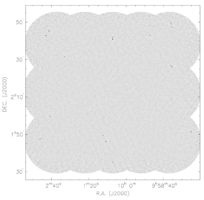
Figure 1.— The VLA-COSMOS Deep image at 2.5^′′ resolution.

Figure 2.— Distribution of the noise in the VLA-COSMOS Deep mosaic. Pixel values extracted from a $52^{\prime}\times 52^{\prime}$ box centered on the COSMOS field center show a Gaussian distribution in agreement with our assumption of Gaussian noise. The fitted Gaussian (dashed line) has a rms of $\rm 12.09\,\mu Jy/beam$ ($\sigma$). The tail at high flux densities is consistent with the presence of sources in the image which were not excluded during the extraction process.

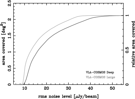
Figure 3.— The rms level vs. the cumulative (left axis) and relative area (right axis) covered by the VLA-COSMOS Large (at a resolution of 1.5${}^{\prime\prime}\times$1.4^′′) and Deep (with a resolution of 2.5${}^{\prime\prime}\times$2.5^′′) project mosaics.

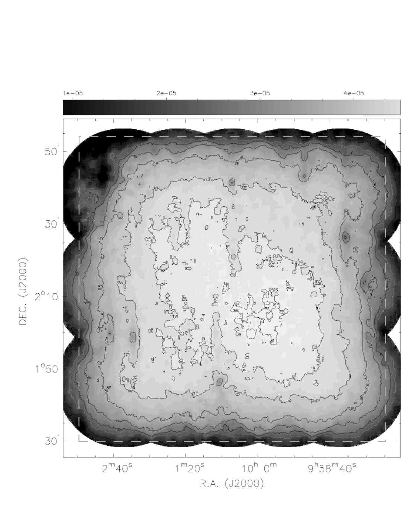
Figure 4.— Sensitivity map of the area covered by the VLA Deep Project, derived using the AIPS task RMSD (see text for details). The rms is fairly uniform except for areas around strong radio sources. Lighter shades indicate lower rms noise values. The contours correspond to rms levels of 10, 12, 15, 20, 25, 30, 34 and 40 $\mu$Jy/beam. The search for radio sources was limited to the area enclosed by the (light grey) 34 $\mu$Jy/beam contour. For comparison, the dashed box indicates the area used to construct the catalog of the Large Project.

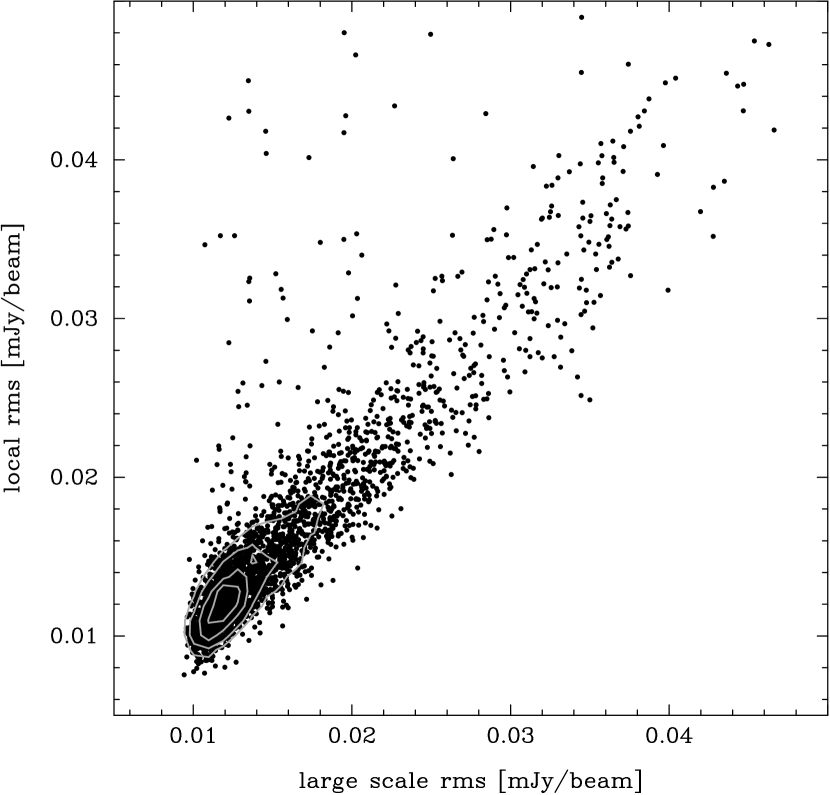
Figure 5.— Comparison of the noise estimate in the rms map used to generate the $S/N$ map for source detection in the 2.5^′′ resolution Deep image (original rms) and in the local rms map generated with a 50 pixel mesh size (corresponding to 17.5^′′). Contours illustrate the distribution of points in the most densely populated part of the scatter plot.

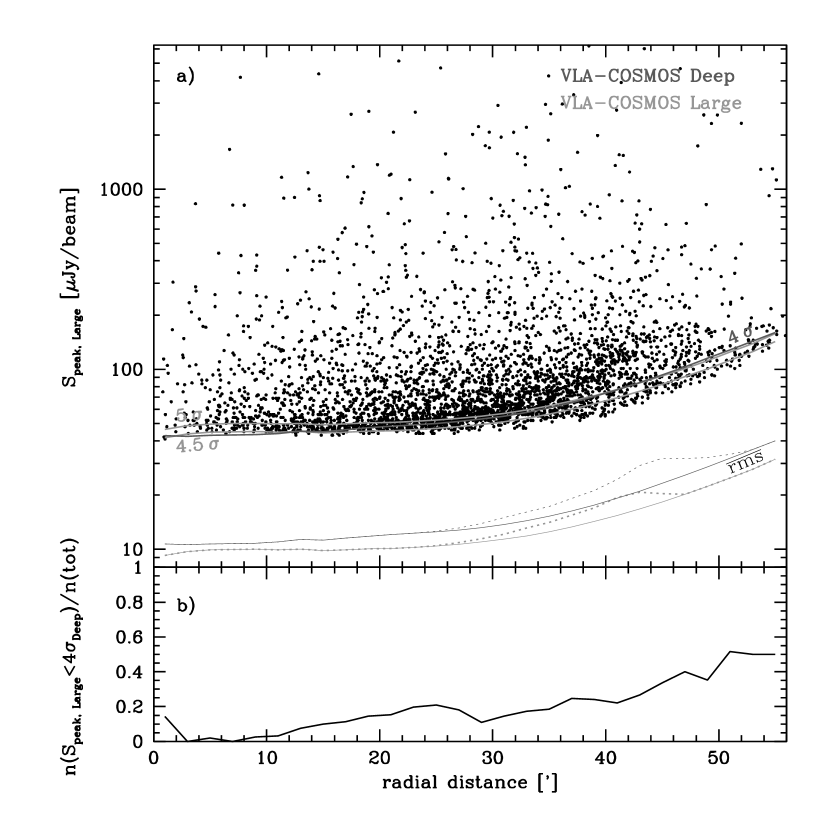
Figure 6.— Correspondence of the detection thresholds used for the Deep and Large catalog. a) Peak flux densities from the Large catalog (v1.0) are compared to the mean rms noise level (${\rm\overline{rms}}$, averaged in concentric rings of width 2^′), and the detection thresholds applied in the VLA-COSMOS Large (light grey curves) and Deep mosaics (dark grey curve). A cubic spline fit to the measured ${\rm\overline{rms}}$ around the bump at $r\approx$ 45^′ gives an estimate of the minimal average noise level at a given radial distance from the center (solid lines at the bottom of the panel). b) Fraction of sources in the Large catalog (v1.0) at a given radial distance $r$ that have a $S/N$ smaller than 4 $\sigma_{\rm Deep}$ in the Deep mosaic.

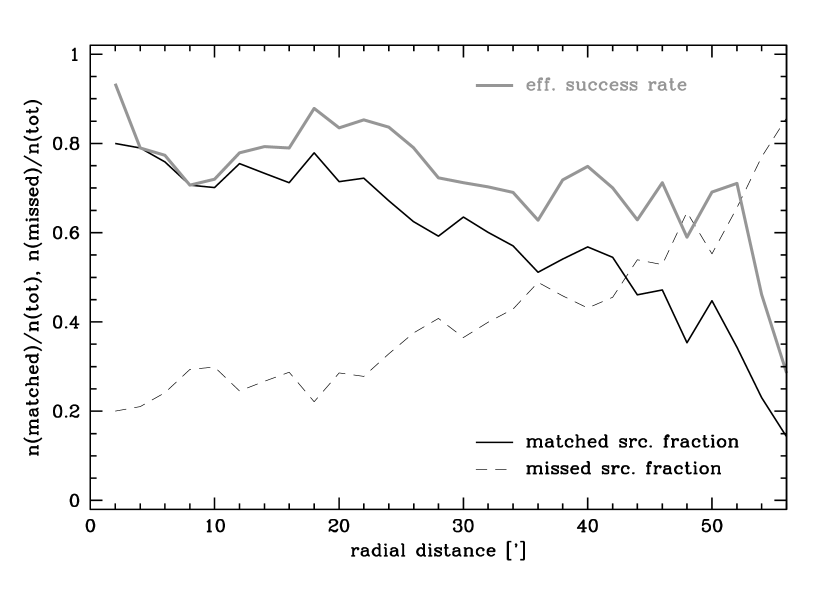
Figure 7.— Fraction of sources in the VLA-COSMOS Large catalog (v1.0) which could (solid black line) or could not (dashed black line) be successfully assigned a counterpart within 1.5^′′ in the VLA-COSMOS Deep catalog. The effective success rate (grey line) is determined by accounting for the fraction of sources that lie below 4$\sigma$ in the Deep image (cf. panel (b) of Fig. 6.) and thus cannot be included in the Deep catalog. The vertical axis is normalized to the total number of sources in the catalog that lie in a given concentric ring of width 2^′.

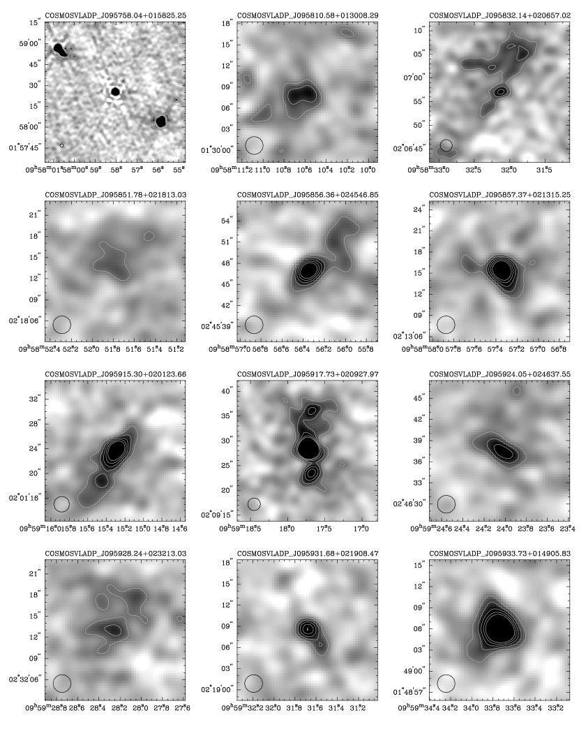
Figure 8.— See last panel of figure for explanations.

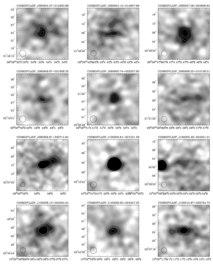
Figure 8.— cont.

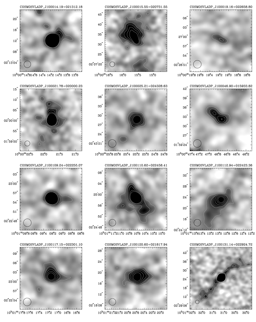
Figure 8.— cont.

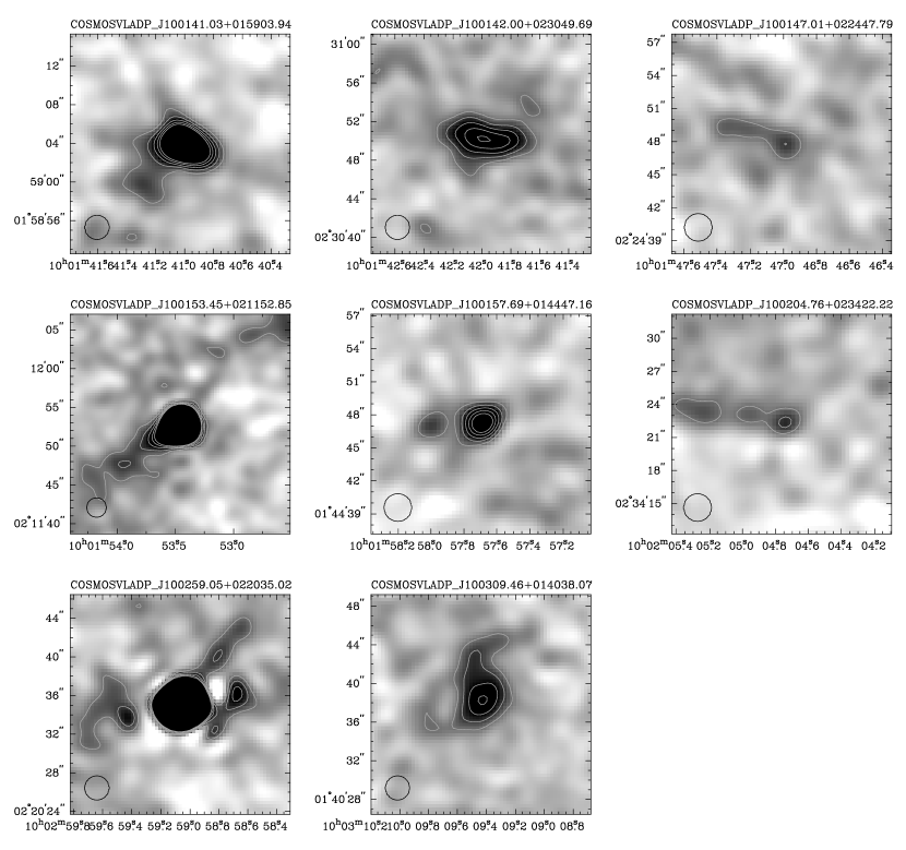
Figure 8.— cont. Radio sources newly fitted with multiple Gaussian components in the VLA-COSMOS Deep image (cf. Fig. 16 of Schinnerer et al. (2007) for images of all previously identified multi-component sources). The source name is specified at the top of the individual panels. The grey-scale ranges from -2$\sigma$ to 7$\sigma$ of the local rms (Tab. 3). The contours start at 3$\sigma$ and increase to a maximum of 11$\sigma$ in steps of 2$\sigma$. The circular beam with FWHM of 2.5^′′ is shown for reference in the lower left corner of each panel.

Figure 9.— Distribution of the ‘local’ $S/N$ measure, $S/N_{17.5^{\prime\prime}}$, for sources present only in the Large (top) or Deep (bottom) catalog. The highest measured $S/N_{17.5^{\prime\prime}}$ was adopted for each source (i.e. the larger of the two $S/N$ values determined at 1.5^′′ or 2.5^′′ resolution, $S/N_{17.5^{\prime\prime}}[1.5^{\prime\prime}]$ and $S/N_{17.5^{\prime\prime}}[2.5^{\prime\prime}]$, respectively). All sources with $S/N_{17.5^{\prime\prime}}\geq 5$ have been included in the Joint catalog. Grey histograms show the distribution of objects which are only detected at 2.5^′′ resolution and for which the detection threshold is only reached in the rms box of 17.5^′′ (flag ‘det’ equals 2 in the Joint catalog; see Table 3 and end of Section 5.2.1 for additional explanations), but not in the 105^′′ rms box used for the initial source extraction in the Deep mosaic.

Figure 10.— Spatial distribution of sources in the VLA-COSMOS Joint catalog that were either not listed in the Deep (light grey) or Large catalog (v1.0) (dark grey). The size of the sign scales with the significance of the detection (see scheme at right). Note that the newly identified bright sources along the eastern and western edge of the field did not figure in the VLA-COSMOS Large project catalog as the search area was previously restricted to the nominal size of the COSMOS field (see Fig. 4). This geometric restriction was dropped in the detection of sources in the mosaic of the Deep Project.

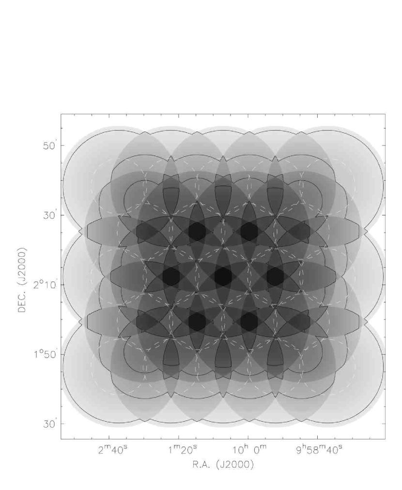
Figure 11.— Model map used for the correction of the bandwidth smearing effect. The model map is based on the sensitivity drop due to the shape of the primary beam response. The intensity scale is normalized to the sensitivity at the center of the field. The contour levels are at 0.1, 0.3, 0.5, 0.7 and 0.9. The area used to extract sources (r $\leq$ 8^′) in each individual pointing for the analysis of Section 6.1 is indicated with dashed white circles.

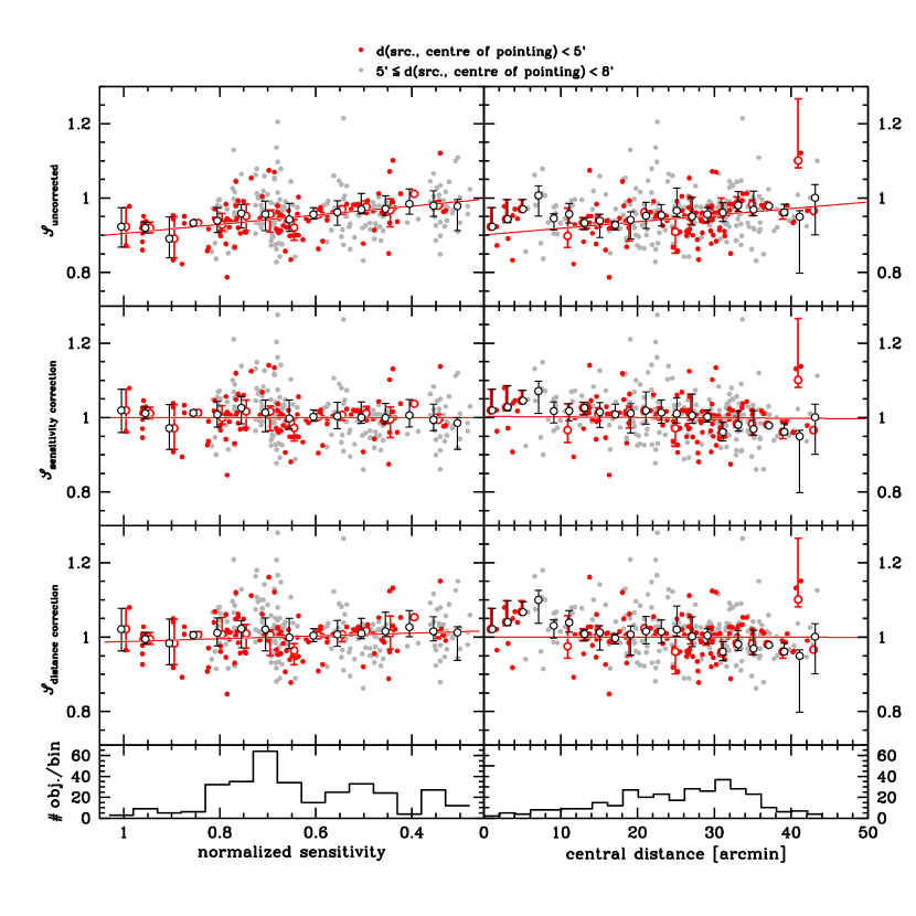
Figure 12.— Comparison of two different approaches to correct for the bandwidth smearing (BWS) effect. (See text for details)

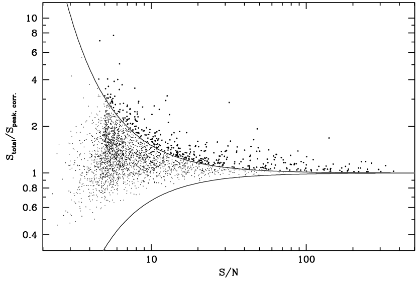
Figure 13.— Ratio of total $S_{\rm total}$ and peak flux density $S_{\rm peak,\,corr.}$ (BWS corrected) as a function of the detection $S/N$, defined as the ratio of the (uncorrected) peak flux density and the local (17.5^′′ box) rms. The solid lines show the upper and lower envelope of the region defined to contain unresolved sources (small dots), based on the simulations presented in the Appendix. Sources lying above the upper envelope are considered resolved (large dots).

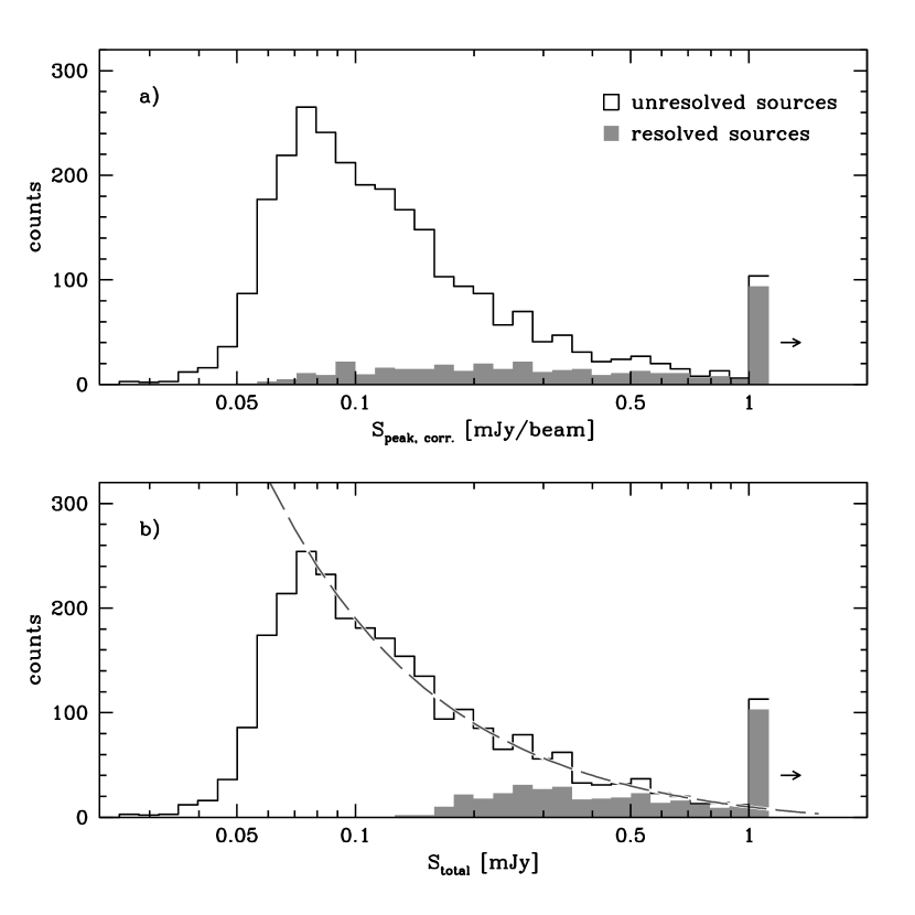
Figure 14.— Number distribution of unresolved and resolved sources in the VLA-COSMOS Joint catalog as a function of corrected peak (top) and integrated flux density (bottom). Sources with $S_{\rm peak,\,corr.}$ or $S_{\rm total}>$ 1 mJy are added to the right-most bin of the histograms. In panel (b) the dashed line (normalized to the counts at 0.1 mJy) illustrates the decline of the integral sources counts $\sim$$S_{\rm total}^{-1}$ which is expected from the flat part of the Euclidan source counts present at low flux levels (e.g. Bondi et al., 2008).

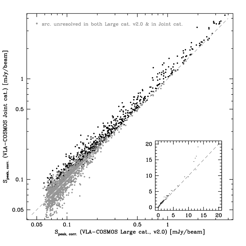
Figure 15.— Comparison of the peak flux densities $S_{\rm peak}$ (both BWS corrected) in the VLA-COSMOS Large (v2.0) and Joint catalog. The inset covers the entire range of peak flux densities while the main part of the figure is limited to peak flux densities less than 4 mJy/beam. The measured values of sources classified as unresolved in both the Large (v2.0) as well as the Joint catalog are in good agreement (grey dots). Sources classified as resolved in the Joint catalog tend to have larger values, as the Deep image has a higher sensitivity to extended emission.

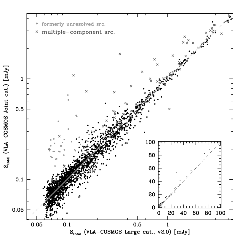
Figure 16.— Comparison of the integrated flux $S_{\rm total}$ in the VLA-COSMOS Large (v2.0) and Joint catalog (the layout of the figure matches that of 15). The majority of the multi-component sources (dark grey crosses) have larger measured integrated fluxes in the Joint catalog as the Deep mosaic is more sensitive to extended emission. Most other sources lie along the diagonal bisector of the plot (indicating a good correspondence between the catalogs), except for sources that were previously classified as unresolved in the Large catalog (v2.0) and are now classified as resolved in the VLA-COSMOS Joint catalog (light grey points).

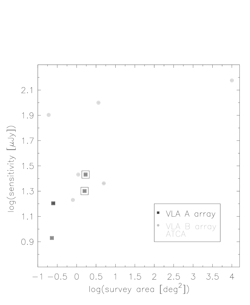
Figure 17.— Comparison of representative radio surveys conducted at 20 cm with the VLA and ATCA. Filled squares denote surveys that were conducted in the VLA A configuration reaching resolutions of $\approx$2^′′, while surveys having resolutions of 5-10^′′ (from the VLA B array and ATCA) are shown as filled circles. The VLA-COSMOS surveys are marked by open squares (Deep: top, Large: bottom), showing that they cover the largest area at their resolution and sensitivity. In order to reasonably compare the different surveys, we used the sensitivity that is achieved for at least 80% of the area covered. Thus in the case of surveys that have a non-uniform rms pattern the sensitivity value used here can be significantly higher than the best value present in the deepest part of the images (for detailed numbers see Tab. 4).

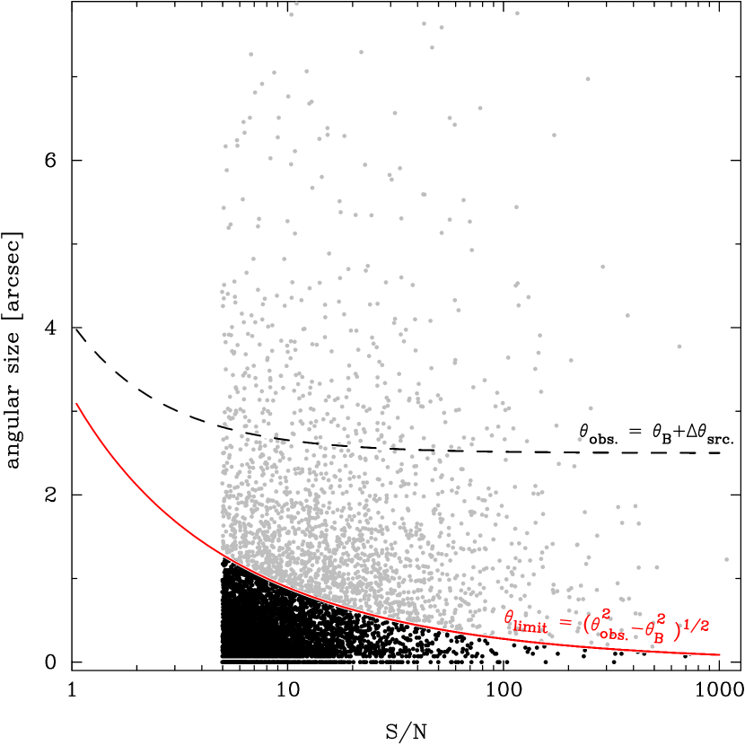
Figure 18.— Intrinsic source sizes of simulated Gaussian sources vs. their detection $S/N$. The dashed line marks the upper expectation value $\theta_{\rm obs.}$ of the observed size of a point source of varying $S/N$ in the Deep mosaic. At low $S/N$, point sources may be significantly larger than the beam size, $\theta_{\rm B}$. The intrinsic (deconvolved) source size, $\theta_{\rm limit}$, inferred from the dashed line is shown in red. It defines an upper limit to the intrinsic source size below which a conclusive classification as resolved or unresolved is no longer possible. Potentially resolvable simulated sources are plotted in grey for easier identification in Fig. 19.

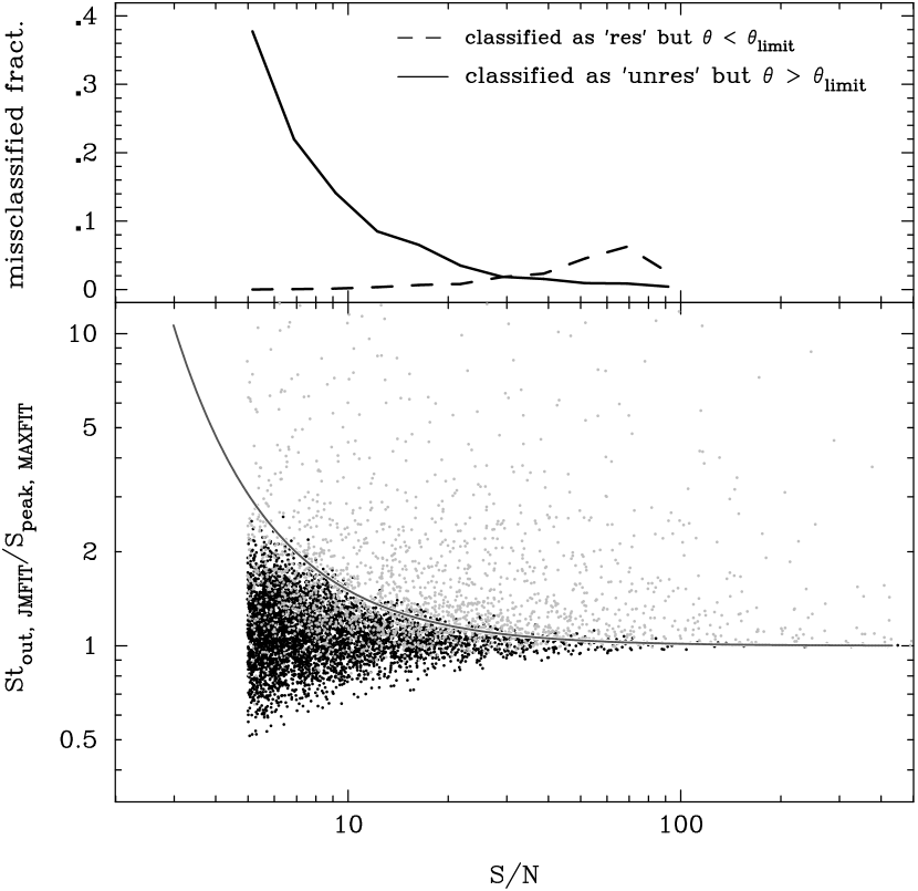
Figure 19.— Diagnostic diagrams for the separation of simulated Gaussian sources into resolved and unresolved objects based on their location in Fig. 18 (see text for details). The color of the dots matches that used in Fig. 18.
In the upper panel we show the fraction of sources in a given bin of $S/N$ that (1) have an intrinsic source size $\theta$ $<$ $\theta_{\rm limit}$ but which nevertheless come to lie above the curve – given by eq. (A2; see lower panel) – separating resolved (above curve) from unresolved (below curve) sources, or (2) have $\theta$ $>$ $\theta_{\rm limit}$ but are found in the area attributed to unresolved objects. (The curves are discontinued at $S/N$ $=$ 100 because small number fluctuations dominate beyond this value.)

Figure 20.— Comparison of the recovered total flux density $St_{\rm out}$ of simulated Gaussian sources with the input value, $St_{\rm in}$. Top row: distribution of relative errors (right) and plot of the relative errors as a function of signal-to-noise ratio (SNR; left) for all simulated sources after these have been classified as resolved or unresolved using eq. (A2). (See also Fig. 19.) Bottom row: close-up of the simulated sources in the bin with the smallest simulated $S/N$.
Total flux densities tend to be overestimated by an amount that increases towards lower $S/N$. The according average bias is listed in Tab. 5 for resolved sources as well as for the complete sample of resolved and unresolved simulated sources.

Table 1VLA Pointing Centers for VLA-COSMOS Deep Project

Pointing #	R.A. (J2000)	DEC (J2000)
F07	10:00:58.62	+02:25:20.42
F08	09:59:58.58	+02:25:20.42
F11	10:01:28.64	+02:12:21.00
F12	10:00:28.60	+02:12:21.00
F13	09:59:28.56	+02:12:21.00
F16	10:00:58.62	+01:59:21.58
F17	09:59:58.58	+01:59:21.58

Note. — The naming convention of the VLA-COSMOS Large project (Schinnerer et al., 2007) has been kept for the pointing centers of the VLA-COSMOS Deep project at 1.4 GHz.

Table 2Source Numbers in the VLA-COSMOS catalogs

Catalog	Type	# of objects	Remarks
Deep Project	components	3744	4$\sigma$ ($\sim$45 $\mu$Jy); total
Deep Project	sources	3441	4$\sigma$ ($\sim$45 $\mu$Jy); total
Large Project (v1.0)	sources	3643	4.5$\sigma$; total
		1226	$<5\sigma$
Large Project (v2.0)	sources	2417	5$\sigma$ ($\sim$60 $\mu$Jy); total
		1611	unresolved sources
		806	resolved sources
		78	multi-component sources
Joint	sources	2865	total; combined Large (v2.0) and Deep Project
		2159	detected in both Large (v1.0) and Deep image
		392	from Large Project (v2.0) catalog
		314	from Deep Project source catalog
		2329	unresolved sources
		405	resolved sources
		131	multi-component sources (incl. 43 new ones)

Note. — See text for details.

Table 31.4 GHz Joint Source Catalog of the VLA-COSMOS Project (abridged)

Name	former Name	R.A.	Dec.	R.A.	Dec.	$\rm\sigma_{R.A.}$	$\rm\sigma_{Dec.}$
	(in Large Project catalog, v2)	[deg], (J2000.0)	[deg], (J2000.0)	(J2000.0)	(J2000.0)	[′′]	[′′]
COSMOSVLADP_J095821.65+024628.1	COSMOSVLA_J095821.65+024628.1	149.5902208	2.7744972	09 58 21.653	+02 46 28.19	0.25	0.25
COSMOSVLADP_J095821.78+024820.6	COSMOSVLA_J095821.78+024820.6	149.5907833	2.8057333	09 58 21.788	+02 48 20.64	0.35	0.36
COSMOSVLADP_J095821.81+014550.7	COSMOSVLA_J095821.82+014550.8	149.5908875	1.7640944	09 58 21.813	+01 45 50.74	0.38	0.41
COSMOSVLADP_J095821.82+014724.1	COSMOSVLA_J095821.81+014724.2	149.5909333	1.7900389	09 58 21.824	+01 47 24.14	0.26	0.26
COSMOSVLADP_J095821.94+020707.7	COSMOSVLA_J095821.94+020707.7	149.5914333	2.1188167	09 58 21.944	+02 07 07.74	0.27	0.27
COSMOSVLADP_J095822.11+014058.9	COSMOSVLA_J095822.10+014058.7	149.5921333	1.6830278	09 58 22.112	+01 40 58.90	0.29	0.27
COSMOSVLADP_J095822.18+014524.3	COSMOSVLA_J095822.18+014524.3	149.5924333	1.7567500	09 58 22.184	+01 45 24.30	0.29	0.30
COSMOSVLADP_J095822.25+013512.3	COSMOSVLA_J999999.99+999999.9	149.5927083	1.5867500	09 58 22.250	+01 35 12.30	0.44	0.38
COSMOSVLADP_J095822.30+024721.3	COSMOSVLA_J095822.30+024721.3	149.5929250	2.7892583	09 58 22.302	+02 47 21.33	-99.00	-99.00
COSMOSVLADP_J095822.57+020239.1	COSMOSVLA_J095822.57+020239.1	149.5940667	2.0441972	09 58 22.576	+02 02 39.11	0.27	0.29
COSMOSVLADP_J095822.81+023604.3	COSMOSVLA_J095822.81+023604.5	149.5950583	2.6012000	09 58 22.814	+02 36 04.32	0.48	0.43
COSMOSVLADP_J095822.93+022619.8	COSMOSVLA_J095822.93+022619.8	149.5955667	2.4388333	09 58 22.936	+02 26 19.80	-99.00	-99.00
COSMOSVLADP_J095823.25+020859.4	COSMOSVLA_J095823.25+020859.4	149.5969083	2.1498417	09 58 23.258	+02 08 59.43	-99.00	-99.00
COSMOSVLADP_J095823.27+021455.9	COSMOSVLA_J095823.27+021455.5	149.5969917	2.2488639	09 58 23.278	+02 14 55.91	0.39	0.35
COSMOSVLADP_J095823.67+021201.4	COSMOSVLA_J095823.68+021201.4	149.5986333	2.2004000	09 58 23.672	+02 12 01.44	0.29	0.31
COSMOSVLADP_J095824.02+024916.0	COSMOSVLA_J095824.02+024916.0	149.6000833	2.8211167	09 58 24.020	+02 49 16.02	-99.00	-99.00
COSMOSVLADP_J095824.02+025029.5	COSMOSVLA_J095824.02+025029.3	149.6000875	2.8415333	09 58 24.021	+02 50 29.52	0.26	0.26
COSMOSVLADP_J095824.13+013836.6	COSMOSVLA_J095824.14+013836.6	149.6005542	1.6435250	09 58 24.133	+01 38 36.69	0.29	0.31

Note. — VLA-COSMOS Joint Catalog of radio sources at 1.4 GHz representing all reliable radio sources from the Large catalog and a search for sources in the Deep mosaic (see text for details). All measurements were made on the 2.5${}^{\prime\prime}\times$2^′′ Deep image. The complete table is available via the link to a machine-readable version above and/or at the COSMOS archive at IPAC/IRSA. A portion is shown here as an example of its form and content.

Table 3cont.

$\rm S_{peak}$	$\rm S_{peak,corr.}\tablenotemark{a}$	$\rm S_{total}$	rms	$\rm\theta_{M,\,dec}$	$\rm\theta_{m,\,dec}$	$\rm PA_{dec}$	Flags
[mJy/beam]	[mJy/beam]	[mJy]	[mJy/beam]	[′′]	[′′]	[∘]	res	mult	memb	det
5.218$\pm$0.029	5.218	5.218$\pm$0.029	0.029	0.00	0.00	0.00	-1	0	0	0
0.201$\pm$0.035	0.201	0.201$\pm$0.035	0.035	0.00	0.00	0.00	0	0	-1	0
0.079$\pm$0.018	0.081	0.081$\pm$0.018	0.018	0.00	0.00	0.00	0	0	0	-1
0.267$\pm$0.014	0.274	0.328$\pm$0.034	0.014	1.43	0.97	60.80	1	0	0	0
0.179$\pm$0.016	0.182	0.182$\pm$0.016	0.016	0.00	0.00	0.00	0	0	0	0
0.154$\pm$0.016	0.154	0.154$\pm$0.016	0.016	0.00	0.00	0.00	0	0	0	0
0.181$\pm$0.017	0.185	0.341$\pm$0.057	0.017	3.04	1.99	94.80	1	0	0	0
0.135$\pm$0.026	0.135	0.135$\pm$0.026	0.026	0.00	0.00	0.00	-2	0	1	1
-99.000	-99.000	30.120	0.083	35.97	9.90	-99.00	1	1	0	-99
0.153$\pm$0.017	0.157	0.157$\pm$0.017	0.017	0.00	0.00	0.00	0	0	0	0
0.093$\pm$0.019	0.096	0.096$\pm$0.019	0.019	0.00	0.00	0.00	0	0	0	-1
-99.000	-99.000	116.500	0.033	74.99	12.92	-99.00	1	1	0	-99
-99.000	-99.000	5.025	0.026	9.90	3.75	-99.00	1	1	0	-99
0.077$\pm$0.016	0.079	0.079$\pm$0.016	0.016	0.00	0.00	0.00	0	0	0	-1
0.162$\pm$0.021	0.169	0.162$\pm$0.021	0.021	0.00	0.00	0.00	-1	0	0	0
-99.000	-99.000	56.620	0.067	56.98	13.93	-99.00	1	1	0	-99
0.461$\pm$0.029	0.461	0.461$\pm$0.029	0.029	0.00	0.00	0.00	-1	0	0	0
0.141$\pm$0.018	0.141	0.141$\pm$0.018	0.018	0.00	0.00	0.00	0	0	0	0

Table 4Selected Radio Surveys at 1.4 GHz

Field	Area	rms	Instrument	Reference
	[deg2]	[$\mu$Jy/beam]
VLA-COSMOS (Deep)	1.7	27	VLA-A	this paper
VLA-COSMOS (Large)	1.6	20	VLA-A	Schinnerer et al. 2007
ECDF-S	0.23	8.5	VLA-A	Miller et al. 2008
SSA 13	0.25	16	VLA-A	Fomalont et al. 2006
FIRST	10,000	150	VLA-B	Becker et al. 1995
FLS	5	23	VLA-B	Condon et al. 2003
SXDF	1.1	27	VLA-A	Simpson et al. 2006
VVDS	0.8	17	VLA-B	Bondi et al. 2003
ATHDFS	0.19	80	ATCA	Norris et al. 2005, Huynh et al. 2005
PDS	3.65	100	ATCA	Hopkins et al. 2003

Note. — Radio surveys displayed in Fig. 17. The values listed were derived from figures similar to Fig. 3 presented in the corresponding references, except for The FIRST and FLS surveys where the full areas are used.

Table 5Median of relative error on recovered integrated flux densities for simulated Gaussian sources (see Appendix).

$S/N$ range	$(St_{\rm in}-St_{\rm out})/St_{\rm in}$ (all sources)	($St_{\rm in}-St_{\rm out})/St_{\rm in}$ (resolved sources)
5-6	-0.05$\pm$0.25	-0.17$\pm$0.42
6-7	-0.02$\pm$0.21	-0.28$\pm$0.39
7-8	0.01$\pm$0.17	-0.16$\pm$0.33
8-9	-0.01$\pm$0.17	-0.19$\pm$0.29
9-10	-0.01$\pm$0.15	-0.20$\pm$0.23
10-15	0.01$\pm$0.12	-0.10$\pm$0.18
15-20	0.01$\pm$0.10	-0.08$\pm$0.15

Note. — Errors span the range (+/-) containing 2/3 of the measurements.

References

- Bertoldi et al. (2007) Bertoldi, F., Carilli, C., Aravena, M., Schinnerer, E., Voss, H., Smolčić, V., Jahnke, K., Scoville, N., Blain, A., Menten, K. M., Lutz, D., Brusa, M., Taniguchi, Y., Capak, P., Mobasher, B., Lilly, S., Thompson, D., Aussel, H., Kreysa, E., Hasinger, G., Aguirre, J., Schlaerth, J., & Koekemoer, A. 2007, ApJS, 172, 132
- Bondi et al. (2008) Bondi, M., Ciliegi, P., Schinnerer, E., Smolčić, V., Jahnke, K., Carilli, C., & Zamorani, G. 2008, ApJ, 681, 1129
- Bondi et al. (2003) Bondi, M., Ciliegi, P., Zamorani, G., Gregorini, L., Vettolani, G., Parma, P., de Ruiter, H., Le Fevre, O., Arnaboldi, M., Guzzo, L., Maccagni, D., Scaramella, R., Adami, C., Bardelli, S., Bolzonella, M., Bottini, D., Cappi, A., Foucaud, S., Franzetti, P., Garilli, B., Gwyn, S., Ilbert, O., Iovino, A., Le Brun, V., Marano, B., Marinoni, C., McCracken, H. J., Meneux, B., Pollo, A., Pozzetti, L., Radovich, M., Ripepi, V., Rizzo, D., Scodeggio, M., Tresse, L., Zanichelli, A., & Zucca, E. 2003, A&A, 403, 857
- Bridle & Schwab (1999) Bridle, A. H., & Schwab, F. R. 1999, in Astronomical Society of the Pacific Conference Series, Vol. 180, Synthesis Imaging in Radio Astronomy II, ed. G. B. Taylor, C. L. Carilli, & R. A. Perley, 371–381
- Capak et al. (2007) Capak, P., Aussel, H., Ajiki, M., McCracken, H. J., Mobasher, B., Scoville, N., Shopbell, P., Taniguchi, Y., Thompson, D., Tribiano, S., Sasaki, S., Blain, A. W., Brusa, M., Carilli, C., Comastri, A., Carollo, C. M., Cassata, P., Colbert, J., Ellis, R. S., Elvis, M., Giavalisco, M., Green, W., Guzzo, L., Hasinger, G., Ilbert, O., Impey, C., Jahnke, K., Kartaltepe, J., Kneib, J.-P., Koda, J., Koekemoer, A., Komiyama, Y., Leauthaud, A., Lefevre, O., Lilly, S., Liu, C., Massey, R., Miyazaki, S., Murayama, T., Nagao, T., Peacock, J. A., Pickles, A., Porciani, C., Renzini, A., Rhodes, J., Rich, M., Salvato, M., Sanders, D. B., Scarlata, C., Schiminovich, D., Schinnerer, E., Scodeggio, M., Sheth, K., Shioya, Y., Tasca, L. A. M., Taylor, J. E., Yan, L., & Zamorani, G. 2007, ApJS, 172, 99
- Carilli et al. (2008) Carilli, C. L., Lee, N., Capak, P., Schinnerer, E., Lee, K.-S., McCraken, H., Yun, M. S., Scoville, N., Smolčić, V., Giavalisco, M., Datta, A., Taniguchi, Y., & Urry, C. M. 2008, ApJ, 689, 883
- Carilli et al. (2007) Carilli, C. L., Murayama, T., Wang, R., Schinnerer, E., Taniguchi, Y., Smolčić, V., Bertoldi, F., Ajiki, M., Nagao, T., Sasaki, S. S., Shioya, Y., Aguirre, J. E., Blain, A. W., Scoville, N., & Sanders, D. B. 2007, ApJS, 172, 518
- Condon (1997) Condon, J. J. 1997, PASP, 109, 166
- Condon et al. (2003) Condon, J. J., Cotton, W. D., Yin, Q. F., Shupe, D. L., Storrie-Lombardi, L. J., Helou, G., Soifer, B. T., & Werner, M. W. 2003, AJ, 125, 2411
- Elvis et al. (2009) Elvis, M., Civano, F., Vignali, C., Puccetti, S., Fiore, F., Cappelluti, N., Aldcroft, T. L., Fruscione, A., Zamorani, G., Comastri, A., Brusa, M., Gilli, R., Miyaji, T., Damiani Anton Koekemoer, F., Finoguenov, A., Brunner, H., Urry, C. M., Silverman, J., Mainieri, V., Hasinger, G., Griffiths, R., Carollo, M., Hao, H., Guzzo, L., Blain, A., Calzetti, D., Carilli, C., Capak, P., Ettori, S., Fabbiano, G., Impey, C., Lilly, S., Mobasher, B., Rich, M., Salvato, M., Sanders, D. B., Schinnerer, E., Scoville, N., Shopbell, P., Taylor, J. E., Taniguchi, Y., & Volonteri, M. 2009, ArXiv e-prints
- Fomalont et al. (2006) Fomalont, E. B., Kellermann, K. I., Cowie, L. L., Capak, P., Barger, A. J., Partridge, R. B., Windhorst, R. A., & Richards, E. A. 2006, ApJS, 167, 103
- Greisen (2003) Greisen, E. W. 2003, in Astrophysics and Space Science Library, Vol. 285, Astrophysics and Space Science Library, ed. A. Heck, 109–+
- Hasinger et al. (2007) Hasinger, G., Cappelluti, N., Brunner, H., Brusa, M., Comastri, A., Elvis, M., Finoguenov, A., Fiore, F., Franceschini, A., Gilli, R., Griffiths, R. E., Lehmann, I., Mainieri, V., Matt, G., Matute, I., Miyaji, T., Molendi, S., Paltani, S., Sanders, D. B., Scoville, N., Tresse, L., Urry, C. M., Vettolani, P., & Zamorani, G. 2007, ApJS, 172, 29
- Hopkins et al. (2003) Hopkins, A. M., Afonso, J., Chan, B., Cram, L. E., Georgakakis, A., & Mobasher, B. 2003, AJ, 125, 465
- Huynh et al. (2005) Huynh, M. T., Jackson, C. A., Norris, R. P., & Prandoni, I. 2005, AJ, 130, 1373
- Ivison et al. (2007) Ivison, R. J., Chapman, S. C., Faber, S. M., Smail, I., Biggs, A. D., Conselice, C. J., Wilson, G., Salim, S., Huang, J.-S., & Willner, S. P. 2007, ApJ, 660, L77
- Ko (1964) Ko, H. C. 1964, IEEE Transactions on Military Electronics, 8, 225
- Koekemoer et al. (2007) Koekemoer, A. M., Aussel, H., Calzetti, D., Capak, P., Giavalisco, M., Kneib, J.-P., Leauthaud, A., Le Fèvre, O., McCracken, H. J., Massey, R., Mobasher, B., Rhodes, J., Scoville, N., & Shopbell, P. L. 2007, ApJS, 172, 196
- Lilly et al. (2007) Lilly, S. J., Le Fèvre, O., Renzini, A., Zamorani, G., Scodeggio, M., Contini, T., Carollo, C. M., Hasinger, G., Kneib, J.-P., Iovino, A., Le Brun, V., Maier, C., Mainieri, V., Mignoli, M., Silverman, J., Tasca, L. A. M., Bolzonella, M., Bongiorno, A., Bottini, D., Capak, P., Caputi, K., Cimatti, A., Cucciati, O., Daddi, E., Feldmann, R., Franzetti, P., Garilli, B., Guzzo, L., Ilbert, O., Kampczyk, P., Kovac, K., Lamareille, F., Leauthaud, A., Borgne, J.-F. L., McCracken, H. J., Marinoni, C., Pello, R., Ricciardelli, E., Scarlata, C., Vergani, D., Sanders, D. B., Schinnerer, E., Scoville, N., Taniguchi, Y., Arnouts, S., Aussel, H., Bardelli, S., Brusa, M., Cappi, A., Ciliegi, P., Finoguenov, A., Foucaud, S., Franceschini, R., Halliday, C., Impey, C., Knobel, C., Koekemoer, A., Kurk, J., Maccagni, D., Maddox, S., Marano, B., Marconi, G., Meneux, B., Mobasher, B., Moreau, C., Peacock, J. A., Porciani, C., Pozzetti, L., Scaramella, R., Schiminovich, D., Shopbell, P., Smail, I., Thompson, D., Tresse, L., Vettolani, G., Zanichelli, A., & Zucca, E. 2007, ApJS, 172, 70
- Miller et al. (2008) Miller, N. A., Fomalont, E. B., Kellermann, K. I., Mainieri, V., Norman, C., Padovani, P., Rosati, P., & Tozzi, P. 2008, ApJS, 179, 114
- Muxlow et al. (2005) Muxlow, T. W. B., Richards, A. M. S., Garrington, S. T., Wilkinson, P. N., Anderson, B., Richards, E. A., Axon, D. J., Fomalont, E. B., Kellermann, K. I., Partridge, R. B., & Windhorst, R. A. 2005, MNRAS, 358, 1159
- Norris et al. (2005) Norris, R. P., Huynh, M. T., Jackson, C. A., Boyle, B. J., Ekers, R. D., Mitchell, D. A., Sault, R. J., Wieringa, M. H., Williams, R. E., Hopkins, A. M., & Higdon, J. 2005, AJ, 130, 1358
- Otoshi (1981) Otoshi, T. Y. 1981, Telecommunications and Data Acquisition Progress Report, 64, 168
- Owen & Morrison (2008) Owen, F. N., & Morrison, G. E. 2008, AJ, 136, 1889
- Prandoni et al. (2000) Prandoni, I., Gregorini, L., Parma, P., de Ruiter, H. R., Vettolani, G., Wieringa, M. H., & Ekers, R. D. 2000, A&AS, 146, 41
- Richards (2000) Richards, E. A. 2000, ApJ, 533, 611
- Sanders et al. (2007) Sanders, D. B., Salvato, M., Aussel, H., Ilbert, O., Scoville, N., Surace, J. A., Frayer, D. T., Sheth, K., Helou, G., Brooke, T., Bhattacharya, B., Yan, L., Kartaltepe, J. S., Barnes, J. E., Blain, A. W., Calzetti, D., Capak, P., Carilli, C., Carollo, C. M., Comastri, A., Daddi, E., Ellis, R. S., Elvis, M., Fall, S. M., Franceschini, A., Giavalisco, M., Hasinger, G., Impey, C., Koekemoer, A., Le Fèvre, O., Lilly, S., Liu, M. C., McCracken, H. J., Mobasher, B., Renzini, A., Rich, M., Schinnerer, E., Shopbell, P. L., Taniguchi, Y., Thompson, D. J., Urry, C. M., & Williams, J. P. 2007, ApJS, 172, 86
- Schinnerer et al. (2004) Schinnerer, E., Carilli, C. L., Scoville, N. Z., Bondi, M., Ciliegi, P., Vettolani, P., Le Fèvre, O., Koekemoer, A. M., Bertoldi, F., & Impey, C. D. 2004, AJ, 128, 1974
- Schinnerer et al. (2007) Schinnerer, E., Smolčić, V., Carilli, C. L., Bondi, M., Ciliegi, P., Jahnke, K., Scoville, N. Z., Aussel, H., Bertoldi, F., Blain, A. W., Impey, C. D., Koekemoer, A. M., Le Fevre, O., & Urry, C. M. 2007, ApJS, 172, 46
- Scott et al. (2008) Scott, K. S., Austermann, J. E., Perera, T. A., Wilson, G. W., Aretxaga, I., Bock, J. J., Hughes, D. H., Kang, Y., Kim, S., Mauskopf, P. D., Sanders, D. B., Scoville, N., & Yun, M. S. 2008, MNRAS, 385, 2225
- Scoville et al. (2007a) Scoville, N., Abraham, R. G., Aussel, H., Barnes, J. E., Benson, A., Blain, A. W., Calzetti, D., Comastri, A., Capak, P., Carilli, C., Carlstrom, J. E., Carollo, C. M., Colbert, J., Daddi, E., Ellis, R. S., Elvis, M., Ewald, S. P., Fall, M., Franceschini, A., Giavalisco, M., Green, W., Griffiths, R. E., Guzzo, L., Hasinger, G., Impey, C., Kneib, J.-P., Koda, J., Koekemoer, A., Lefevre, O., Lilly, S., Liu, C. T., McCracken, H. J., Massey, R., Mellier, Y., Miyazaki, S., Mobasher, B., Mould, J., Norman, C., Refregier, A., Renzini, A., Rhodes, J., Rich, M., Sanders, D. B., Schiminovich, D., Schinnerer, E., Scodeggio, M., Sheth, K., Shopbell, P. L., Taniguchi, Y., Tyson, N. D., Urry, C. M., Van Waerbeke, L., Vettolani, P., White, S. D. M., & Yan, L. 2007a, ApJS, 172, 38
- Scoville et al. (2007b) Scoville, N., Aussel, H., Brusa, M., Capak, P., Carollo, C. M., Elvis, M., Giavalisco, M., Guzzo, L., Hasinger, G., Impey, C., Kneib, J.-P., LeFevre, O., Lilly, S. J., Mobasher, B., Renzini, A., Rich, R. M., Sanders, D. B., Schinnerer, E., Schminovich, D., Shopbell, P., Taniguchi, Y., & Tyson, N. D. 2007b, ApJS, 172, 1
- Seymour et al. (2004) Seymour, N., McHardy, I. M., & Gunn, K. F. 2004, MNRAS, 352, 131
- Simpson et al. (2006) Simpson, C., Martínez-Sansigre, A., Rawlings, S., Ivison, R., Akiyama, M., Sekiguchi, K., Takata, T., Ueda, Y., & Watson, M. 2006, MNRAS, 372, 741
- Smolčić et al. (2008) Smolčić, V., Schinnerer, E., Scodeggio, M., Franzetti, P., Aussel, H., Bondi, M., Brusa, M., Carilli, C. L., Capak, P., Charlot, S., Ciliegi, P., Ilbert, O., Ivezić, Ž., Jahnke, K., McCracken, H. J., Obrić, M., Salvato, M., Sanders, D. B., Scoville, N., Trump, J. R., Tremonti, C., Tasca, L., Walcher, C. J., & Zamorani, G. 2008, ApJS, 177, 14
- Smolčić et al. (2009a) Smolčić, V., Schinnerer, E., Zamorani, G., Bell, E. F., Bondi, M., Carilli, C. L., Ciliegi, P., Mobasher, B., Paglione, T., Scodeggio, M., & Scoville, N. 2009a, ApJ, 690, 610
- Smolčić et al. (2009b) Smolčić, V., Zamorani, G., Schinnerer, E., Bardelli, S., Bondi, M., Birzan, L., Carilli, C. L., Ciliegi, P., Ilbert, O., Koekemoer, A. M., Merloni, A., Paglione, T., Salvato, M., Scodeggio, M., & Scoville, N. 2009b, ArXiv e-prints
- Taniguchi et al. (2007) Taniguchi, Y., Scoville, N., Murayama, T., Sanders, D. B., Mobasher, B., Aussel, H., Capak, P., Ajiki, M., Miyazaki, S., Komiyama, Y., Shioya, Y., Nagao, T., Sasaki, S. S., Koda, J., Carilli, C., Giavalisco, M., Guzzo, L., Hasinger, G., Impey, C., LeFevre, O., Lilly, S., Renzini, A., Rich, M., Schinnerer, E., Shopbell, P., Kaifu, N., Karoji, H., Arimoto, N., Okamura, S., & Ohta, K. 2007, ApJS, 172, 9
- Thompson (1999) Thompson, A. R. 1999, in Astronomical Society of the Pacific Conference Series, Vol. 180, Synthesis Imaging in Radio Astronomy II, ed. G. B. Taylor, C. L. Carilli, & R. A. Perley, 11–36
- Trump et al. (2007) Trump, J. R., Impey, C. D., McCarthy, P. J., Elvis, M., Huchra, J. P., Brusa, M., Hasinger, G., Schinnerer, E., Capak, P., Lilly, S. J., & Scoville, N. Z. 2007, ApJS, 172, 383
- Wells (1981) Wells, D. The Penguin Dictionary of Curious and Interesting Geometry, London: Penguin Books, pp. 30-31, 1991
- Windhorst et al. (1984) Windhorst, R. A., van Heerde, G. M., & Katgert, P. 1984, A&AS, 58, 1
- Zamojski et al. (2007) Zamojski, M. A., Schiminovich, D., Rich, R. M., Mobasher, B., Koekemoer, A. M., Capak, P., Taniguchi, Y., Sasaki, S. S., McCracken, H. J., Mellier, Y., Bertin, E., Aussel, H., Sanders, D. B., Le Fèvre, O., Ilbert, O., Salvato, M., Thompson, D. J., Kartaltepe, J. S., Scoville, N., Barlow, T. A., Forster, K., Friedman, P. G., Martin, D. C., Morrissey, P., Neff, S. G., Seibert, M., Small, T., Wyder, T. K., Bianchi, L., Donas, J., Heckman, T. M., Lee, Y.-W., Madore, B. F., Milliard, B., Szalay, A. S., Welsh, B. Y., & Yi, S. K. 2007, ApJS, 172, 468