Asymptotic profiles for a travelling front solution of a biological equation

Abstract

We are interested in the existence of depolarization waves in the human brain. These waves propagate in the grey matter and are absorbed in the white matter. We consider a two-dimensional model $u_{t}=\Delta u+f(u)\mathbbm{1}_{|y|\leq R}-\alpha u\mathbbm{1}_{|y|>R}$, with $f$ a bistable nonlinearity taking effect only on the domain $\mathbb{R}\times[-R,R]$, which represents the grey matter layer. We study the existence, the stability and the energy of non-trivial asymptotic profiles of possible travelling fronts. For this purpose, we present dynamical systems technics and graphic criteria based on Sturm-Liouville theory and apply them to the above equation. This yields three different behaviours of the solution $u$ after stimulation, depending of the thickness $R$ of the grey matter. This may partly explain the difficulties to observe depolarization waves in the human brain and the failure of several therapeutic trials.
Keywords: spreading depression, reaction-diffusion equation, travelling fronts, Sturm-Liouville theory.
AMS classification codes (2000): 34C10, 35B35, 35K57, 92C20.

1 Introduction

The propagation of depolarization waves, also called spreading depressions, may appear in a brain during strokes, migraines with aura or epilepsy. In rodent brains, the propagation of depolarization waves has been observed for more than fifty years [15]. During stroke in rodent brain, they cause important damages and are therefore a therapeutic target. Pharmacological agents blocking the appearance of those waves have been studied and reduce strongly after-effects of stroke in the rodent brain [18, 19]. However propagation of depolarization waves during stroke in the human brain is still uncertain [1, 16, 17, 23, 24] and the pharmalogical agents used in rodent have seemed to have no effect on human stroke. Mathematical models of these depolarization waves may help to understand these points.

In [2], the first author has build a mathematical model of these waves and has studied numerically how the morphology of the brain may influence their propagation. Simplifications of the mathematical model lead to the study of propagation phenomena for the following biological equation

$$\frac{\partial u}{\partial t}-\triangle u=f(u)\mathbbm{1}_{\Omega}-\alpha u\mathbbm{1}_{\mathbb{R}^{N}\setminus\Omega},\qquad t\in\mathbb{R},\,X\in\mathbb{R}^{N},$$ (1.1)

where $f(u)=\lambda\;u(u-a)(1-u)$ is the usual bistable nonlinearity with $a\in]0,1/2[$ and $\lambda>0$, and where $\alpha$ is a positive number. We denote by $\mathbbm{1}_{\Omega}$ the caracteristic function of the domain $\Omega$ that is $\mathbbm{1}_{\Omega}(X)=1$ if $X\in\Omega$ and $\mathbbm{1}_{\Omega}(X)=0$ elsewhere. The function $u$ represents the depolarization of the brain that is that if $u(X)=0$ the brain is normally polarized at the point $X$ whereas if $u(X)=1$ the brain is totally depolarized. The domain $\Omega$ represents the grey matter of a brain, where the reaction-diffusion process that triggers depolarization waves takes place, whereas $\mathbb{R}^{N}\setminus\Omega$ contains the white matter, where the waves are absorbed. The problem is to understand the influence of the geometry of $\Omega$ on the propagation of waves. In particular, the layer of grey matter in the human brain is thiner than in other species and admits more circumvolutions. The influence of the circumvolutions of the grey matter is partially studied in [4].

We will focus here on the influence of the thickness of the layer of grey matter. We may assume that $\Omega$ is a straight cylinder of radius $2R$. In [2], numerical studies have shown that small values of $R$ may prevent the spreading of the ionic waves. A partial theoretical study in any dimension $N$ has been led in [3], where the first author has proved the non-existence of the depolarization waves if the thickness $R$ is small enough and their existence if $R$ is large enough.

The results of [3] are not completely satisfactory. First, they only deal with $R$ small or large enough. Secondly, no complete description of the possible asymptotic profiles of the travelling waves, their stability, or their energy, has been pursued. As a consequence, even if the existence of waves is proved, nothing is known about their asymptotic profiles and their stability. The purpose of the present paper is to complete this study for any $R$, in dimension $N=2$. More precisely, we consider the equation

$$\frac{\partial u}{\partial t}=\triangle u+f(u)\mathbbm{1}_{|y|\leq R}-\alpha u\mathbbm{1}_{|y|>R},\qquad t\in\mathbb{R},\,(x,y)\in\mathbb{R}^{2}~{}.$$ (1.2)

We are looking to solutions travelling in the $x$ direction at speed $c$, that are solutions $u$ of (1.2) which can be written $u(x,y,t)=v(x-ct,y)$. Travelling fronts are solutions $u(x,y,t)=v(x-ct,y)$ such that there are two asymptotic profiles $V_{-}\neq V_{+}$ with $\lim_{\xi\rightarrow\pm\infty}\|v(\xi,.)-V_{\pm}\|_{H^{1}(\mathbb{R})}=0$. Using standard elliptic estimates, a profile $V$ is a solution in $H^{1}(\mathbb{R})$ of the equation

$$V^{\prime\prime}+f(V)\mathbbm{1}_{|y|\leq R}-\alpha V\mathbbm{1}_{|y|>R}=0,~{}~{}~{}y\in\mathbb{R}~{}.$$ (1.3)

Notice that a profile is trivially associated to an equilibrium point $E(x,y)=V(y)$ that is a stationnary solution of (1.2). The trivial equilibrium point $E\equiv 0$ corresponds to the normal state of the brain, whereas a non-trivial equilibrium point corresponds to a depolarized state, deleterious for the brain. We are more particularly interested in the existence of travelling fronts with positive speed $c$ connecting the profile $V_{+}\equiv 0$ with a non-trivial profile $V_{-}$. Such fronts correspond to the invasion of the equilibrium state $0$ by a deleterious state.

The purpose of this article is to achieve a complete study of the existence of the profiles, their stability and their energy (see the following sections for the definitions of stability and energy).

Main result 1.1.

There exist two critical thicknesses $R_{1}>R_{0}>0$ such that:
i) if $0<R<R_{0}$, there is no non-trivial profile, i.e. that $V\equiv 0$ is the only solution of (1.3) in $H^{1}(\mathbb{R})$.
ii) If $R_{0}<R$, there exist non-trivial profiles. One of them, denoted by $V_{M}$, is larger than every other one. The largest profile $V_{M}$ is stable, and every other non-trivial profiles are unstable.
iii) The energy of the unstable profiles is always larger than the energy of the stable profiles $0$ and $V_{M}$. If $R_{0}<R<R_{1}$, the energy of $V_{M}$ is larger than the energy of $0$, whereas it is smaller if $R>R_{1}$.

In this paper, we first adapt several graphic criteria for stability of profiles, based on Sturm-Liouville theory. Then, we present dynamical systems technics for studying energy of profiles. These criteria and technics are general ones and are valid for any nonlinearity $f$. We obtain the above results by applying these ideas to the particular nonlinearity $f(u)=\lambda\;u(u-a)(1-u)$. The check on the graphic criteria sometimes relies on a numerical study of the phase plane.

Once the profiles and their stability completely described by the Main Result 1.1, one is able to obtain the existence of travelling fronts.

Consequences 1.2.

 
i) If $0<R<R_{0}$ then there is no travelling front for Equation (1.2).
ii) If $R_{0}<R<R_{1}$ there exists a globally stable travelling front $u(x,y,t)=v(x-ct,y)$ with $\lim_{\xi\rightarrow+\infty}v(\xi,.)=0$ and $\lim_{\xi\rightarrow-\infty}v(\xi,.)=V_{M}$ with a negative speed $c<0$.
ii) If $R_{1}<R$ there exists a globally stable travelling front $u(x,y,t)=v(x-ct,y)$ with $\lim_{\xi\rightarrow+\infty}v(\xi,.)=0$ and $\lim_{\xi\rightarrow-\infty}v(\xi,.)=V_{M}$ with a positive speed $c>0$.

Assertion i) is a clear consequence of the Main Result 1.1. The proof that this Main Result also implies the other assertions is not the goal of this paper and will not be detailled. One way to prove it is to use a method recently introduced by Risler in [20]. The fundamental idea is to use the existence of an energy functional for (1.2) in any Galilean frame travelling at constant speed $s$ in the $x$ direction. Keeping this basic idea, the original proof has been revised in [10] and [9]. The adaptation of these technics to Equation (1.2) has been detailled in [3]. The original motivation of Risler’s technics was to develop a method of proof of existence and stability of fronts in equations where no comparison principle is available. As suggested by the work of the first author in [3], the method of Risler is also usefull to get the existence and stability of fronts in equations as (1.2) for which even if there is a comparison principle, no particular positive subsolution is known.

The results of this article yield a good insight into the different behaviours of the depolarization in the grey matter after it has been stimulated. If the stimulation takes place in a part of a brain where the grey matter is thin ($R<R_{0}$), the neurons of the grey matter quickly repolarize, i.e. the solution of (1.2) goes back to zero, uniformly and exponentially fast. If the grey matter is slightly thicker ($R_{0}<R<R_{1}$), the repolarization is slower and more progressive, the depolarized area disappearing by shrinking. Mathematically speaking, there exists a stable non-trivial profile but with an energy larger than zero. Thus, the equilibrium state zero invades the excited state by travelling fronts, reducing the excited area. Notice that it may take very long time to go back to rest if the initial excited area is large. Finally, if the grey matter is thick ($R_{1}<R$), a depolarization wave propagates. Indeed, the excited state has a lower energy than zero. These three behaviours are illustrated in Figure 1. The fact that the behaviour depends on the width of the grey matter may explain why the depolarization waves have been observed or not in the human brain depending on the experiments, see [1, 16, 17] or[24] and the discussion of Section 5.

Figure 1: The three typical behaviours of the depolarization in the grey matter after stimulation. From left to right: $R<R_{0}$, $R_{0}<R<R_{1}$ and $R_{1}<R$.

The paper is splitted as follows. In Section 2 we explicit a relation between the profiles and the equilibrium points of a parabolic equation in $(-R,R)$. In Section 3, we obtain graphic criteria of existence and stability of the profiles, mainly based on Sturm-Liouville theory. The energy of the different profiles is studied in Section 4, using technics coming from the infinite dimensional dynamical systems theory. Finally, in Section 5, we discuss the relations between our mathematical results and the biological phenomena of spreading waves in the brains.

2 Relations with a parabolic equation on $(-R,R)$

In this preliminary section, we enhance an obvious relation between the profiles and the equilibrium points of a parabolic equation on the segment $(-R,R)$. We also recall some basic properties of the dynamics of this parabolic equation. In fact, in this paper, we could perform all the arguments with the parabolic equation on the whole domain $\mathbb{R}$. However, this would bring useless technicalities.

2.1 Back to a bounded interval

The profiles $V$ are the solutions of Equation (1.3). In other word, they are the stationnary solutions of the evolution equation

$$\frac{\partial u}{\partial t}=\frac{\partial^{2}u}{\partial y^{2}}+g(y,u)$$ (2.1)

where $g(y,u)=f(u)\mathbbm{1}_{|y|\leq R}-\alpha u\mathbbm{1}_{|y|>R}$. The energy corresponding to this reaction-diffusion equation is the functional $E:H^{1}(\mathbb{R})\longrightarrow\mathbb{R}$ defined by

$$E(u)=\frac{1}{2}\int_{\mathbb{R}}\left|\frac{du}{dy}(y)\right|^{2}dy~{}-~{}\int_{\mathbb{R}}G(y,u(y))dy$$ (2.2)

where $G(y,u)=\int_{0}^{u}g(y,v)dv$ is a primitive of $g$.

We notice that any profile $V$ satisfies $V(y)=c_{+}e^{\sqrt{\alpha}y}+c_{-}e^{-\sqrt{\alpha}y}$ outside $(-R,R)$. Since $V$ belongs to $H^{2}(\mathbb{R})$, one has $c_{+}=0$ for $y>R$ and $c_{-}=0$ for $y<R$. Since $H^{2}(\mathbb{R})\subset\mathcal{C}^{1}(\mathbb{R})$, $V$ is continuous and solving (1.3) is equivalent to solving the following problem

$$\left\{\begin{array}[]{ll}V^{\prime\prime}(y)+f(V(y))=0&~{}~{}y\in(-R,R)\\ V^{\prime}(-R)=\sqrt{\alpha}\;V(-R)&\\ V^{\prime}(R)=-\sqrt{\alpha}\;V(R)~{}.&\end{array}\right.$$ (2.3)

Equation (2.3) caracterises the equilibrium points of a parabolic equation on $(-R,R)$ with Robin boundary conditions

$$\left\{\begin{array}[]{ll}\displaystyle\frac{\partial u}{\partial t}(y,t)=\frac{\partial^{2}u}{\partial y^{2}}(y,t)+f(u(y,t))&~{}~{}(y,t)\in(-R,R)\times\mathbb{R}_{+}\\ \displaystyle\frac{\partial u}{\partial y}(-R,t)=\sqrt{\alpha}\;u(-R,t)&~{}~{}t>0\\ \displaystyle\frac{\partial u}{\partial y}(R,t)=-\sqrt{\alpha}\;u(R,t)&~{}~{}t>0\end{array}\right.$$ (2.4)

The energy corresponding to Equation (2.4) is given by

$$\mathcal{E}(u)=\frac{1}{2}\int_{-R}^{R}\left|\frac{du}{dy}(y)\right|^{2}dy~{}-~{}\int_{-R}^{R}F(u(y))dy+\frac{\sqrt{\alpha}}{2}\left(|u(R)|^{2}+|u(-R)|^{2}\right)$$ (2.5)

where $F(u)=\int_{0}^{u}f(v)dv$ is a primitive of $f$.

It is straightforward to verify that if $V$ is a profile, then $E(V)=\mathcal{E}(V_{|(-R,R)})$. As a conclusion, the problems of the existence and the energy of the profiles are equivalent to the study of the equilibrium points of the parabolic equation (2.4) and their energy. We will often abusively denote $V_{|(R,R)}$ by simply $V$. However, notice that the dynamics of the equation (2.1) on the whole real line and the ones of (2.4) on $(-R,R)$ are different. Moreover, the spectrum of the linearization of (2.1) at a profile $V$ is different from the spectrum of the linearization of (2.4) at $V_{|(-R,R)}$, even if we prove in Section 3.2 that the number of positive eigenvalues is the same.

2.2 Basic facts about the parabolic equation on $(-R,R)$

The theory of the parabolic equation (2.4) with Robin boundary conditions is very well-known, see for example [14]. We recall here some basic dynamical properties, which will be used in this paper.

First, (2.4) admits a comparison principle.

Lemma 2.1.

Let $u(t)$ and $v(t)$ be two solutions of (2.4) with respective initial data $u_{0}$ and $v_{0}$ belonging to $H^{1}(-R,R)$. Assume that $u_{0}(y)\leq v_{0}(y)$ for all $y\in(-R,R)$. Then, for all $(y,t)\in(-R,R)\times\mathbb{R}_{+}$, $u(y,t)\leq v(y,t)$.

Secondly, the parabolic type of (2.4) and the fact that $f(u)u<0$ for large $u$ implies that any solution $u(t)$ with initial data $u_{0}\in H^{1}(-R,R)$ is bounded in $H^{k}(-R,R)$ uniformly for $t\in[t_{0},+\infty)$ for any $t_{0}>0$ and for any $k\in\mathbb{N}$. This yields a compacity result.

Lemma 2.2.

Let $(t_{n})_{n\in\mathbb{N}}$ be a sequence of times such that $\liminf t_{n}>0$, let $(u^{0}_{n})_{n\in\mathbb{N}}\subset H^{1}(-R,R)$ be a sequence of initial data and let $u_{n}(t)$ be the solutions of (2.4) with $u_{n}(0)=u_{n}^{0}$.
Then, there exist an extraction $\varphi$ and a function $u_{\infty}\in H^{1}(-R,R)$ such that $\|u_{\varphi(n)}(t_{\varphi(n)})-u_{\infty}\|_{H^{1}(-R,R)}\longrightarrow 0$ when $n$ goes to $+\infty$.

The energy $\mathcal{E}$ defined by (2.5) is a strict Lyapounov functional for the dynamics of (2.4): for each $u(t)\in H^{1}(-R,R)$ solution of (2.4), the function $\mathcal{E}(u(t))$ is decreasing in time, except if $u(t)$ is constant, that is except if $u$ is an equilibrium point, and thus a profile. Indeed, it is straightforward to get $\partial_{t}\mathcal{E}(u(t))=-\int_{-R}^{R}|\frac{\partial u}{\partial t}(y,t)|^{2}dt$. The existence of a strict Lyapounov function yields what is called gradient dynamics. In addition of the compacity property of Lemma 2.2, it is very classical to obtain Lasalle principle, see [13].

Lemma 2.3.

Let $u(t)$, $t\geq 0$, be a solution in $H^{1}(-R,R)$ of (2.4). Let $\omega(u)$ be the $\omega-$limit set of $u$, that is

$$\omega(u)=\left\{v\in H^{1}(-R,R)~{}/~{}\exists(t_{n})_{n\in\mathbb{N}},~{}t_{n}\xrightarrow[n\rightarrow+\infty]{}+\infty~{}\text{ and }~{}\|u(t_{n})-v\|_{H^{1}(-R,R)}\xrightarrow[n\rightarrow+\infty]{}0\right\}~{}.$$

Then, $\omega(u)$ is a non-empty connected compact set which only consists in equilibrium points, i.e. in profiles.
Similarly, if $u(t)$ is defined for all $t\in\mathbb{R}$ and uniformly bounded, the $\alpha-$limit set

$$\alpha(u)=\left\{v\in H^{1}(-R,R)~{}/~{}\exists(t_{n})_{n\in\mathbb{N}},~{}t_{n}\xrightarrow[n\rightarrow+\infty]{}-\infty~{}\text{ and }~{}\|u(t_{n})-v\|_{H^{1}(-R,R)}\xrightarrow[n\rightarrow+\infty]{}0\right\}~{}$$

is a non-empty connected compact set which only consists in profiles. Moreover, if $V_{-}\in\alpha(u)$ and $V_{+}\in\omega(u)$ then $\mathcal{E}(V_{-})>\mathcal{E}(V_{+})$ and in particular $V_{-}\not\equiv V_{+}$.

3 Existence and stability of profiles

We are interested in the asymptotic profiles of the possible travelling fronts of Equation (1.2). We recall that a profile $V\in H^{1}(\mathbb{R})$ is solution of (1.3). We wonder if there exist non-trivial profiles (i.e. profiles $V\not\equiv 0$) and if they are stable. A profile $V$ is stable if the linear operator $L_{V}:H^{2}(\mathbb{R})\longrightarrow L^{2}(\mathbb{R})$ defined by

$$L_{V}\varphi=\varphi^{\prime\prime}+\left(f^{\prime}(V)\mathbbm{1}_{|y|\leq R}-\alpha\mathbbm{1}_{|y|>R}\right)\varphi$$ (3.1)

has no spectrum in the half-plane $\{z\in\mathcal{C},Re(z)\geq 0\}$.

In this section, we give graphic criteria for existence and stability of profiles and we apply them to Equation (1.3) to obtain the following result.

Proposition 3.1.

For any given $\alpha$, $\lambda$ and $a$, there exists a positive number $R_{0}$ such that:
i) if $R<R_{0}$, then there does not exist any profile different from $0$.
ii) if $R\geq R_{0}$, then there exist non-trivial profiles. One of them, denoted by $V_{M}$ is strictly larger than every others, smaller than $1$ and is even. Moreover, if $R>R_{0}$ then $V_{M}$ and $0$ are stable profiles and are the only ones to be stable.
iii) if $\alpha\geq a\lambda$ then if $R>R_{0}$, there exist exactly two non-trivial profiles.

3.1 A graphic criterium for existence of profiles

We recall here the simple graphic arguments already mentionned in [3]. As already noticed, looking for profiles $V$ solutions of (1.3) is equivalent to looking for solutions $V$ of the equation (2.3). In the phase plane, the flow $\Phi_{y_{0}}:\mathbb{R}^{2}\longrightarrow\mathbb{R}^{2}$ associated to the differential equation $V^{\prime\prime}+f(V)=0$ between $-R$ and $y_{0}$ is given by

$$\Phi_{y_{0}}(V_{0},V_{1})=(V(y_{0}),V^{\prime}(y_{0}))~{}~{}\text{ where }V\text{ solves }~{}~{}\left\{\begin{array}[]{l}V^{\prime\prime}(y)+f(V(y))=0~{},~{}~{}y\in(-R,y_{0})\\ (V(-R),V^{\prime}(-R))=(V_{0},V_{1})\end{array}\right.$$

Let $\mathcal{D}$ and $\mathcal{D}^{\prime}\subset\mathbb{R}^{2}$ be the straight lines $\mathbb{R}.(1,\sqrt{\alpha})$ and $\mathbb{R}.(1,-\sqrt{\alpha})$. Notice that the conditions $V^{\prime}(-R)=\sqrt{\alpha}\;V(-R)$ and $V^{\prime}(R)=-\sqrt{\alpha}\;V(R)$ correspond to $(V,V^{\prime})(-R)\in\mathcal{D}$ and $(V,V^{\prime})(R)\in\mathcal{D}^{\prime}$ respectively. Hence, the graphic interpretation of (2.3) is the following.

Graphic criterium 3.2.

The profiles, i.e. the solutions of (2.3), correspond to the trajectories of the flow $\Phi_{y}$ that start on $\mathcal{D}$ when $y=-R$ and finish on $\mathcal{D}^{\prime}$ when $y=R$. Therefore, they correspond to the intersections of the curve $\Phi_{R}\mathcal{D}$ with the straight line $\mathcal{D}^{\prime}$.

The results of existence stated in Proposition 3.1 follow from Graphic Criterium 3.7. The critical radius $R_{0}$ is the first (positive) $R$ such that $\Phi_{R}\mathcal{D}$ intersects $\mathcal{D}^{\prime}$ elsewhere than at $(0,0)$. In Figures 2 and 3, we illustrate the phase plane, the flow $\Phi_{y}$ and the curve $\Phi_{R}\mathcal{D}$ for different cases. Figure 4 shows the graph of four profiles $V(y)$ in $[-R,R]$ and the corresponding intersections in the phase plane.

Figure 2: The phase plane for $\alpha\geq a\lambda$ and $\Phi_{R}\mathcal{D}$ for three increasing values of $R$: two cases with no non-trivial profiles and the last with two non-trivial profiles.

Figure 3: The phase plane for $\alpha<a\lambda$ and $\Phi_{R}\mathcal{D}$ for three increasing values of $R$: no non-trivial profiles, two ones and four ones.

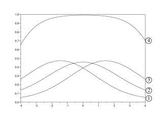
Figure 4: The intersections of $\Phi_{R}\mathcal{D}$ and $\mathcal{D}^{\prime}$ in the phase plane and the corresponding profiles in the $(y,V)$ plane

Figures 2 and 3 show that there are two cases. If $\mathcal{D}$ is always outside the domain delimited by the homoclinic orbit to zero, then there cannot exist more than two non-trivial profiles. If $\mathcal{D}$ intersects the homoclinic orbit to zero, then for $R$ large enough there exist as much non-trivial profiles as wanted. The critical value of $\alpha$ is obtained by computing the unstable direction of $0$ in the phase plane. This direction is given by the eigenvector $(1,\sqrt{a\lambda})$ related to the eigenvalue $\sqrt{a\lambda}$ of the matrix $\left(\begin{array}[]{cc}0&1\\ a\lambda&0\end{array}\right)$, which corresponds to the linearization of the flow at the equilibrium point $(0,0)$. This shows that $\mathcal{D}$ intersects the homoclinic orbit to zero if and only if $\alpha<a\lambda$.

The fact that there exists a profile $V_{M}$ larger than the other ones is classical, see for example [21]. It is a consequence of Lemmas 2.1 and 2.3: if $u(t)$ is a solution of (2.4) with $u(0)$ larger than any profile, then the $\omega-$limit set $\omega(u(0))$ consists in a profile $V_{M}$ larger than any profile. The fact that $V_{M}$ is even follows from the symmetry of the problem since $V_{M}(-.)$ is also a profile. Notice that this symmetry corresponds to the symmetry of the phase plane and to the fact that the trajectory $y\mapsto\Phi_{y}(V_{M}(-R),V^{\prime}_{M}(-R))$ intersect $\mathcal{D}^{\prime}$ for the first time at $y=R$.

3.2 A graphic criterium for stability of the profiles

Let $V$ be a profile solution of (1.3). We consider the linearization $L_{V}$ of the flow along the profile $V$. We recall that $L_{V}$ is given by (3.1). The operator $L_{V}$ is self-adjoint and is a relatively compact disturbance of $\Delta-\alpha$ and therefore has the same essential spectrum, see [14]. This yields the following characterisation of the stability of a profile $V$, see [22].

Proposition 3.3.

The spectrum of $L_{V}$ consists in $]-\infty,-\alpha]$ and a finite number of isolated real eigenvalues $\mu_{i}>-\alpha$ of finite multiplicity. As a consequence, the profile $V$ is asymptotically stable if and only if $L_{V}$ has no nonnegative eigenvalue.

We are looking to nonnegative eigenvalues of $L_{V}$ that is to $\lambda\geq 0$ such that there exists $\varphi\in H^{2}(\mathbb{R})$ such that $\varphi\not\equiv 0$ and

$$\varphi^{\prime\prime}(y)+\left(f^{\prime}(V(y))\mathbbm{1}_{|y|\leq R}-\alpha\mathbbm{1}_{|y|>R}\right)\varphi(y)=\mu\varphi(y)~{}.$$ (3.2)

By the same argument used for $V$ in Section 2, $\varphi$ is explicit outside $(-R,R)$ and it is equivalent to look to $\varphi$ satisfying

$$\left\{\begin{array}[]{ll}\varphi^{\prime\prime}(y)+f^{\prime}(V(y))\varphi(y)=\mu\varphi(y)&~{}~{}y\in(-R,R)\\ \varphi^{\prime}(-R)=\sqrt{\mu+\alpha}\varphi(-R)&\\ \varphi^{\prime}(R)=-\sqrt{\mu+\alpha}\varphi(R)&\end{array}\right.$$ (3.3)

In this section, we adapt the standard Sturm-Liouville theory to the eigenvalue problem (3.3). Keeping in mind the geometric interpretation of Sturm-Liouville arguments, we will obtain a graphic criterium to count the number of nonnegative eigenvalues of $L_{V}$. The idea of using such graphic arguments for studying the one-dimensional parabolic equation is not new, see [8]. In fact, one can understand the whole dynamics of a one-dimensional parabolic equation by similar arguments as shown in [6]. See for example [7] for a review on this subject.

For any $\mu\geq 0$ we define $\theta_{\mu}$ by

$$\left\{\begin{array}[]{l}\theta_{\mu}^{\prime}=-\sin^{2}\theta_{\mu}+\left(\mu-f^{\prime}(V(y))\right)\cos^{2}\theta_{\mu}~{}~{},~{}~{}~{}y\in(-R,R)\\ \theta_{\mu}(-R)=\arctan(\sqrt{\mu+\alpha})\end{array}\right.$$ (3.4)

and we set for $\mu>-\alpha$

$$h(\mu)=\theta_{\mu}(R)+\arctan(\sqrt{\mu+\alpha})~{}.$$ (3.5)

Lemma 3.4.

A nonnegative number $\mu$ is a nonnegative eigenvalue of $L_{V}$ if and only if $h(\mu)$ belongs to $\pi\mathbb{Z}$.

Proof: Let $\mu\geq 0$ and $\varphi\in\mathcal{C}^{2}([-R,R])$, $\varphi\not\equiv 0$, satisfying (3.3). We introduce two functions of class $\mathcal{C}^{2}$, $\rho>0$ and $\theta\in\mathbb{R}$, such that $(\varphi,\varphi^{\prime})(y)=\rho(y)(\cos\theta(y),\sin\theta(y))$. Notice that these functions exist and are regular since the vector $(\varphi,\varphi^{\prime})$ cannot vanish because $\varphi$ is a non-trivial solution of a linear second-order differential equation. Up to the change of the sign of $\varphi$ and to the addition of a constant in $\pi\mathbb{Z}$ to $\theta$, $\varphi^{\prime}(-R)=\sqrt{\mu+\alpha}\varphi(-R)$ implies $\theta(-R)=\arctan(\sqrt{\mu+\alpha})$. Moreover, it follows from (3.3) that, for $y\in(-R,R)$,

$$\theta^{\prime} =-\sin^{2}\theta+\left(\mu-f^{\prime}(V(y))\right)\cos^{2}\theta$$

$$\rho^{\prime} =\rho\sin\theta\cos\theta\left(1+\mu-f^{\prime}(V(y))\right)$$ (3.6)

Hence, $\theta=\theta_{\mu}$ and $\varphi^{\prime}(R)=-\sqrt{\mu+\alpha}\varphi(R)$ is equivalent to $\theta_{\mu}=-\arctan(\sqrt{\mu+\alpha})+k\pi$ with $k\in\mathbb{Z}$.
To show the other implication, it is sufficient to follow the previous arguments in the opposite way: we start with a function $\theta_{\mu}$, we construct $\rho$ by (3.6) and we check that $\varphi=\rho\cos\theta_{\mu}$ is a solution of (3.3). $\square$

Lemma 3.5.

Let $V$ be a profile solution of (1.3).
i) If $\mu>\|f^{\prime}(V)\|_{\infty}$ then, for all $y\in[-R,R]$, $\theta_{\mu}(y)\in(0,\frac{\pi}{2})$ and $h(\mu)\in(0,\pi)$.
ii) If $\mu_{1}>\mu_{2}$ then, for all $y\in[-R,R]$, $\theta_{\mu_{1}}(y)>\theta_{\mu_{2}}(y)$ and $h$ is an increasing function.

Proof: We prove assertion i) by contradiction. Let $y_{0}=\inf\{y\in[-R,R]/\theta_{\mu}(y)\not\in(0,\pi/2)\}$. Notice that $y_{0}>-R$ since $\theta_{\mu}(-R)\in(0,\pi/2)$. If $\theta_{\mu}(y_{0})=0$, then $\theta^{\prime}_{\mu}(y_{0})=\mu-f^{\prime}(V(y_{0}))>0$ which is absurd since $\theta_{\mu}(y)>0$ for $y<y_{0}$ by definition of $y_{0}$. The contradiction is similar if $\theta_{\mu}(y_{0})=\pi/2$.
The proof of ii) is very similar: let $y_{0}=\inf\{y\in[-R,R]/\theta_{\mu_{1}}(y)\leq\theta_{\mu_{2}}(y)\}$. We have $\theta_{\mu_{1}}(y_{0})=\theta_{\mu_{2}}(y_{0})$. If $\theta_{\mu_{1}}(y_{0})\not\in\pi/2+\pi\mathbb{Z}$, then $\theta^{\prime}_{\mu_{1}}(y_{0})-\theta^{\prime}_{\mu_{2}}(y_{0})=(\mu_{1}-\mu_{2})\cos^{2}\theta_{\mu_{1}}(y_{0})>0$ and it contradicts the definition of $y_{0}$. If $\theta_{\mu_{i}}(y_{0})\in\pi/2+\pi\mathbb{Z}$, then $\theta^{\prime}_{\mu_{1}}(y_{0})=\theta^{\prime}_{\mu_{2}}(y_{0})$, $\theta^{\prime\prime}_{\mu_{1}}(y_{0})=\theta^{\prime\prime}_{\mu_{2}}(y_{0})$ and $\theta^{\prime\prime\prime}_{\mu_{1}}(y_{0})=2+\mu_{1}-f^{\prime}(V(y_{0}))>\theta^{\prime\prime\prime}_{\mu_{2}}(y_{0})$. In both cases, we obtain the desired contradiction. $\square$

As a consequence of both preceding lemmas, we obtain the following Sturm-Liouville-type result.

Proposition 3.6.

Let $V$ be a profile solution of (1.3). Let $L_{V}$ be the operator defined by (3.1) and let $h$ be the function defined by (3.5).
i) $k\in\mathbb{N}$ is such that $h(0)\in(-k\pi,(1-k)\pi]$ if and only if the operator $L_{V}$ has $k$ nonnegative eigenvalues.
ii) if $L_{V}$ has a nonnegative eigenvalue, there exists a positive eigenfunction associated to the largest eigenvalue of $L_{V}$.
iii) the nonnegative eigenvalues of $L_{V}$ are simple.

Proof: By Lemma 3.4, the nonnegative eigenvalues correspond to the values $\mu$ for which $h(\mu)\in\mathbb{Z}$. Since, as shown in Lemma 3.5, $\mu\mapsto h(\mu)$ is increasing and belongs to $(0,\pi)$ for large $\mu$, then Assertion i) follows from the continuity of $h$. Moreover, if it exists, the largest eigenvalue $\mu$ is necessary such that $h(\mu)=0$. Thus $\theta_{\mu}(R)\in(-\pi/2,\pi/2)$. Since $\theta_{\mu}(-R)\in(-\pi/2,\pi/2)$ and since $\theta_{\mu}^{\prime}(y)<0$ as soon as $\theta_{\mu}(y)=\pm\pi/2$, we must have $\theta_{\mu}(y)\in(-\pi/2,\pi/2)$ for all $y\in[-R,R]$. Following the arguments in the proof of Lemma 3.4, we construct an associated eigenfunction $\varphi=\rho\cos\theta_{\mu}$ which is positive on $[-R,R]$. It is positive on $\mathbb{R}$ by the extension imposed by (3.2). Finally, the eigenspace of a nonnegative eigenvalue is one-dimensional since any eigenfunction must satisfy (3.3). Since $L_{V}$ is self-adjoint, any nonnegative eigenvalue is simple. $\square$

The interest of the first assertion of Proposition 3.6 is to have a graphic interpretation. Indeed, let $\varphi$ be the solution of $(\varphi,\varphi^{\prime})(-R)=(1,\sqrt{\alpha})$ and $\varphi^{\prime\prime}+f^{\prime}(V)\varphi=0$. In other words, $y\mapsto(\varphi,\varphi^{\prime})(y)$ is a trajectory of the linearization of the flow $D_{V}\Phi_{y}$ along the profile $V$ such that $(\varphi,\varphi^{\prime})(-R)$ is in the tangent space of $\mathcal{D}$ at $(V,V^{\prime})(-R)$. For each $y\in(-R,R)$, $(\varphi,\varphi^{\prime})(y)$ is therefore in the tangent space of $\Phi_{y}\mathcal{D}$ at $(V,V^{\prime})(y)$. By the same arguments as in the proof of Lemma 3.4, $\theta_{0}(y)$ defined by (3.4) is exactly the argument of the vector $(\varphi,\varphi^{\prime})(y)$. Therefore, one can observe the angle $\theta_{0}(y)$ by looking at the argument of the vector tangent to $\Phi_{y}\mathcal{D}$ at $(V,V^{\prime})(y)$. Thus, we can graphically interpret Assertion i) of Proposition 3.6 in the following way.

Graphic criterium 3.7.

Let $V$ be a profile, solution of (1.3) and let $L_{V}$ be the operator defined by (3.1). Let $y\in[-R,R]\longmapsto A_{V}(y)\in\mathbb{R}^{2}$ be a continuous function such that for all $y\in[-R,R]$, $A_{V}(y)$ is a unit vector tangent to $\Phi_{y}\mathcal{D}$ at $(V,V^{\prime})(y)$. Then, the number of times $A_{V}(y)$ crosses the direction of $\mathcal{D}^{\prime}$ when $y$ describes $[-R,R]$ is exactly the number of nonnegative eigenvalues of $L_{V}$. The crossings have to be counted in a algebraic way: positively in the clockwise sense and negatively otherwise.

The previous graphic criterium is illustrated in Figure 5. This criterium requires the knowledge of the curve $\Phi_{y}\mathcal{D}$ for each $y\in(-R,R)$. Therefore, it is difficult to apply as it stands. Fortunately, there is a way to count the number of times $A_{V}(y)$ crosses the direction of $\mathcal{D}^{\prime}$ with the knowledge of the curve $\Phi_{R}\mathcal{D}$ only. Indeed, in the particular case of this article, the phase plane associated to $f$ is such that the curve $\Phi_{R}\mathcal{D}$ is above $\mathcal{D}^{\prime}$ in $\{(u,v)\in\mathbb{R}^{2},~{}u\geq 1\}$ and below $\mathcal{D}^{\prime}$ in $\{(u,v)\in\mathbb{R}^{2},~{}u<0\}$. For this reason, using homotopy and topological arguments, the vectors $A_{0}(y)$ and $A_{V_{M}}(y)$ corresponding to the extremal profiles $0$ and $V_{M}$ must have a trivial number of crossings with the direction of $\mathcal{D}^{\prime}$. Moreover, for another profile $V$, we can compute the number of crossings of $A_{V}(y)$ with $\mathcal{D}^{\prime}$ as follows.

Figure 5: an example of application of the graphic criterium 3.7. One counts along a profile $V$ the number of crossings between the tangent vector to the curve $\Phi_{y}\mathcal{D}$ and the direction of $\mathcal{D}^{\prime}$. This gives the number of nonnegative eigenvalues of $L_{V}$. Left, the largest profile has no nonnegative eigenvalue. Right, the other non-trivial profile has one nonnegative eigenvalue.

Graphic criterium 3.8.

Let $V$ be a given profile. We follow the curve $\Phi_{R}\mathcal{D}$ from $0$ (or from $V_{M}$) to $V$. We count in a algebraic way the number of times the unit tangent vector to $\Phi_{R}\mathcal{D}$ crosses the direction of $\mathcal{D}^{\prime}$ during this course. The resulting number is exactly the number of nonnegative eigenvalues corresponding to the profile $V$.

The equivalence of the graphic criteria 3.7 and 3.8 can be easily “seen on the figure”. However, the rigourous proof uses homotopies and the topology of the plane, similarly to Jordan theorem. This proof is not the subject of this paper and will be omitted.

We can apply the above graphic criterium to the particular phase plane of this article. Because the flow of $V^{\prime\prime}+f(V)$ is turning around the equilibrium $(a,0)$, every profile $V$, which is not one of the extremal profiles $0$ or $V_{M}$, is unstable, see Figure 6.

Figure 6: examples of application of the graphic criterium 3.8. One follows the curve $\Phi_{R}\mathcal{D}$ from $0$ to a profile $V$ and counts in a algebraic way the number of crossings between the tangent vector to the curve and the direction of $\mathcal{D}^{\prime}$. One then obtains the number of nonnegative eigenvalues of $L_{V}$. At the left, the largest profile (2) has no nonnegative eigenvalue whereas the other non-trivial profile (1) has one nonnegative eigenvalue. At the right, the four non-trivial profiles have respectively one, two, one and zero nonnegative eigenvalues.

4 Energy of the profiles

We recall that the relevant energy for the profiles is the function $E$ defined by (2.2). We also recall that the energy $E(V)$ of a profile $V$ is equal to the energy $\mathcal{E}(V_{|(-R,R)})$ of the restriction of $V$ to $(-R,R)$, see Section 2. Let $R_{0}$ be the critical thickness introduced in Proposition 3.1. We know that for $R>R_{0}$ there exists a unique non-trivial profile $V_{M}$ which is stable and that $V_{M}$ is the largest profile. This section is devoted to the following result.

Proposition 4.1.

 
i) If $V$ is an unstable profile, then $E(V)$ is larger than $E(0)=0$ and $E(V_{M})$.
ii) There exists $R_{2}\geq R_{0}$ such that on $(R_{0},R_{2})$ (this set being possibly empty, for example if $\alpha\geq a\lambda$) the energy $E(V_{M})$ of the largest profile is an increasing function of the radius $R$ and on $(R_{2},+\infty)$, $E(V_{M})$ is a decreasing function of the radius $R$.
iii) $E(V_{M})$ is positive for $R>R_{0}$ close to $R_{0}$ and converges to $-\infty$ when $R$ goes to $+\infty$.
As a consequence, there exists a radius $R_{1}>R_{0}$ such that $E(V_{M})$ is positive for $R_{0}<R\leq R_{1}$ and negative for $R>R_{1}$.

The proof of Proposition 4.1 relies on technics which are more general than the framework of this paper. However, to obtain Proposition 4.1 we have to use properties of the phase plane corresponding to (2.3). These particular properties are observed on the phase plane and on the numerical simulations.

4.1 Energy of the unstable profiles

We prove here the first assertion of Proposition 4.1. The proof relies on the following lemma.

Lemma 4.2.

Let $V$ be an unstable profile. Let $\mu>0$ be the first eigenvalue of $L_{V}$ and let $\varphi$ be a positive associated eigenfunction, the existence of which is stated in Proposition 3.6. Then, there exist two globally bounded solutions $u_{-}(t)$ and $u_{+}(t)$ of (2.4) with the following prescribed asymptotic behaviour in $H^{1}(-R,R)$:

$$u_{\pm}(t)=V\pm e^{\mu t}\varphi+o\left(e^{\mu t}\right)~{}~{}~{}\text{when }t\longrightarrow-\infty~{}.$$ (4.1)

As a consequence, for all $(y,t)\in(-R,R)\times\mathbb{R}$, $u_{-}(y,t)\leq V(y)\leq u_{+}(y,t)$.

Proof: The lemma is a classical application of the theory of stable and unstable manifolds near an equilibrium point. We refer to [5] and [14]. Indeed, we can split the spectrum of the linearisation $L_{V}$ into $\{\mu\}$ and the spectrum contained in the half-plane $\{z\in\mathcal{C},~{}\mathrm{Re}(z)\leq\mu-\varepsilon\}$ with $\varepsilon>0$ small enough. As shown in Proposition 3.6, $\mu$ is simple and admits a positive eigenfunction $\varphi$. We defined the strongly unstable set by

$$W^{uu}(V)=\{ u_{0}\in H^{1}(-R,R),~{}\exists~{}u(t)\text{ global solution of \eqref{eq-evo-prof-2} such that}$$

$$\lim_{t\rightarrow-\infty}e^{(-\mu+\varepsilon/2)t}\|u(t)-V\|_{H^{1}(-R,R)}=0~{}\}~{}.$$

The theory of invariant manifolds near an equilibrium point shows that $W^{uu}(V)$ is an invariant one-dimensional manifold which is tangent at $V$ to the line $V+\mathbb{R}\varphi$. The manifold $W^{uu}(V)$ consists in $V$ and two globally defined trajectories $u_{+}$ and $u_{-}$ satisfying the asymptotic behaviour (4.1). Of course, the last assertion is a direct consequence of this asymptotic behaviour, of the positivity of $\varphi$ and of Lemma 2.1. $\square$

The first assertion of Proposition 4.1 is deduced from Lemma 4.2 as follows. Let $V$ be an unstable profile. We know from Section 3 that $V$ lies between $0$ and the largest profile $V_{M}$, both being stable. Let $u_{-}(t)$ be the solution given by Lemma 4.2 for the profile $V$. By Lemma 2.2, the $\omega-$limit set of $u_{-}$ is non-empty and consists in profiles. We wonder which profiles may belong to this $\omega-$limit set. Assume that there is an unstable profile $\tilde{V}$ in $\omega(u_{-})$. This profile must satisfy $\tilde{V}\leq V$ since $u_{-}(t)\leq V$ for all $t$. Moreover, by Lemma 2.3, $\tilde{V}\not\equiv V$ and thus, by uniqueness of ODE solutions, $\tilde{V}(y)<V(y)$ for all $y\in\mathbb{R}$. Let $\tilde{u}_{+}(t)$ be the solution given by Lemma 4.2 for the profile $\tilde{V}$. For $t$ close to $-\infty$, $\tilde{u}_{+}(t)<u_{-}(t)$. Using Lemma 2.1, $\tilde{V}\leq\tilde{u}_{+}(t)\leq u_{-}(t)\leq V$ for all times. Since Lemma 2.3 prevents $\tilde{u}_{+}(t)$ to go back to $\tilde{V}$, $u_{-}(t)$ cannot converge to $\tilde{V}$, which yields a contradiction. Therefore, since $\omega(u_{-})$ is non-empty, the only possibility is $\omega(u_{-})=\{0\}$. Lemma 2.3 then shows that $\mathcal{E}(V)>\mathcal{E}(0)=0$.

By using $u_{+}(t)$, we prove similarly that $\mathcal{E}(V)>\mathcal{E}(V_{M})$. Notice that the above arguments also prove that every unstable profile intersects the other unstable ones as illustrated in Figure 4.

4.2 Energy of the stable profile

The proof of the second and third assertions of Proposition 4.1 is splitted in several parts. We use in this section the notations of Section 3.1 with obvious changes to add the dependence of the different objects with respect to $R$.

$\bullet$ $R\mapsto V^{R}_{M}(0)$ is increasing.
To study the function $R\mapsto V^{R}_{M}$, we invoke the graphic interpretation of the profiles developped in Section 3.1. By symmetry of the largest profile, $V^{R}_{M}(0)$ is the intersection of the trajectory $y\mapsto\Phi_{y}(V^{R}_{M}(-R),\alpha V^{R}_{M}(-R))$ with the horizontal axis. Therefore, $R\mapsto V^{R}_{M}(0)$ is increasing if and only if $R\mapsto V^{R}_{M}(-R)$ is increasing. For $R$ given, $\Phi_{R}(V^{R}_{M}(-R),\alpha V^{R}_{M}(-R))$ belongs to $\mathcal{D}^{\prime}$ and at this point of the phase plane, the flow $\Phi_{y}$ crosses $\mathcal{D}^{\prime}$ transversally from the top to the bottom. Thus, for small $\varepsilon>0$, $\Phi_{R+\varepsilon}(V^{R}_{M}(-R),\alpha V^{R}_{M}(-R))$ is below $\mathcal{D}^{\prime}$ and by continuity, there exists an intersection of $\Phi_{R+\varepsilon}\mathcal{D}$ and $\mathcal{D}^{\prime}$ at the right of $\Phi_{R+\varepsilon}(V^{R}_{M}(-R),\alpha V^{R}_{M}(-R))$. This means that $V^{R+\varepsilon}_{M}(-R-\varepsilon)>V^{R}_{M}(-R)$ and thus $R\mapsto V^{R}_{M}(0)$ is increasing. See Figure 7.

Figure 7: when $R=R_{0}$, a saddle-node bifurcation creates a stable profile $V^{R}_{M}$ (the largest profile) and an unstable profile $V^{R}$. When $R>R_{0}$ increases, the largest profile $V^{R}_{M}$ is increasing. When $R\rightarrow+\infty$ the largest profile $V^{R}_{M}$ piles up to the singularity $(1,0)$ of the phase plane.

By a standard implicit functions argument, one shows that $R\mapsto V^{R}_{M}$ is continuous and differentiable as soon as $\Phi_{R}\mathcal{D}$ intersects $\mathcal{D}^{\prime}$ transversally at $(V^{R}_{M}(R),\alpha V^{R}_{M}(R))$. We admit that it is always the case when $R>R_{0}$.

$\bullet$ $E(V^{R}_{M})$ converges to $-\infty$ when $R$ goes to $+\infty$.
This fact has already been proved in [3] by the first author. We only give here brief arguments. When $R$ increases, the trajectory $y\in(-R,R)\mapsto\Phi_{y}(V^{R}_{M}(-R),\alpha V^{R}_{M}(-R))$ goes to the right and $V^{R}_{M}(0)$ converges to $1$. For large $R$, the trajectory $y\in(-R,R)\mapsto\Phi_{y}(V^{R}_{M}(-R),\alpha V^{R}_{M}(-R))$ spends a time $O(R)$ in a neighborhood of $(1,0)$, where $(u,v)\mapsto\frac{1}{2}|v|^{2}-F(u)$ is negative, and a bounded time outside. Therefore $E(V^{R}_{M})=\mathcal{E}(V^{R}_{M})$ goes to $-\infty$ when $R$ goes to $+\infty$.

$\bullet$ There exists $\beta\in(a,1)$ such that $R\mapsto E_{R}(V^{R}_{M})$ is increasing if $V^{R}_{M}(0)<\beta$ and decreasing if $V^{R}_{M}(0)>\beta$
We admit that for all $R>R_{0}$, $R\mapsto V^{R}_{M}(y)$ is differentiable. Let $E_{\rho}$ be the energy functional defined by (2.2) with $R=\rho$. Let $V$ be a given fixed profile. We consider the variation of $\rho\mapsto E_{\rho}(V)$ at $\rho=R$.

$$\partial_{\rho}E_{\rho}(V)_{|\rho=R}=\left(-F(V(R))-\frac{\alpha}{2}\left|V(R)\right|^{2}\right)+\left(-F(V(-R))-\frac{\alpha}{2}\left|V(-R)\right|^{2}\right)$$

Since $V(\pm R)=\pm\sqrt{\alpha}\;V^{\prime}(\pm R)$ and since $V^{\prime\prime}(y)+f(V(y))=0$, $y\mapsto\frac{1}{2}\left|\partial_{y}V(y)\right|^{2}+F(V(y))$ is constant and

$$\partial_{\rho}E_{\rho}(V)=-2F(V(0))~{}.$$

Since $V$ is an equilibrium of (2.1), it is a critical point for the energy $E_{R}$. In other words, for any $W\in H^{1}(\mathbb{R})$,

$$\partial_{h}E_{R}(V+hW)=0~{}.$$

Henceforth, if $R\mapsto V^{R}_{M}$ is differentiable, then combining both derivatives yields

$$\partial_{R}\left(E_{R}(V^{R}_{M})\right)=-2F(V^{R}_{M}(0))~{}.$$

It remains to notice that $R\mapsto V^{R}_{M}(0)$ is increasing and converges to $1$ when $R$ goes to $+\infty$. Moreover, there exists $\beta>0$ such that $F$ is negative on $(0,\beta)$ and positive on $(\beta,1]$. In fact, $(\beta,0)$ is the point of the phase plane where the homoclinic orbit to 0 intersects the horizontal axis, see Figure 7.

$\bullet$ $E_{R}(V^{R}_{M})$ is positive for $R$ close to $R_{0}$.
When $R$ passes the value $R_{0}$, the creation of both non trivial profiles occurs through a saddle-node bifurcation: two equilibrium states appear at the same point, one stable and one unstable. The stable profile is $V^{R}_{M}$, the largest one, and we denote by $V^{R}$ the unstable profile which lies between $0$ and $V^{R}_{M}$. From now on, we work in $(-R,R)$ by using the analogy presented in Section 2. We want to show that $\mathcal{E}(V^{R}_{M})$ is positive for $R$ close to $R_{0}$. When $R$ decreases to $R_{0}$: the profiles $V_{M}^{R}$ and $V^{R}$ collide. As $\mathcal{E}(V^{R})>0$ for $R>R_{0}$ as shown in Section 4.1, we must have at the limit $\mathcal{E}(V^{R_{0}})=\mathcal{E}(V^{R_{0}}_{M})\geq 0$. Assume that $\mathcal{E}(V^{R_{0}}_{M})=0$. Let $R_{n}>R_{0}$ be a sequence of thickness decreasing to $R_{0}$ and let $V^{R_{n}}$ be the associated unstable profiles. Let $u^{n}_{-}(t)$ be the sequence of solutions of (2.4) given by Lemma 4.2 applied to $V^{R_{n}}$. We know by Section 4.1 that $u^{n}_{-}(t)$ converges to $0$ when $t$ goes to $+\infty$. Let $K=\lim_{n\rightarrow+\infty}\|V^{R_{n}}\|_{H^{1}(-R,R)}$. Notice that $K$ is positive since for each $n$ there exists $y\in(-R,R)$ such that $V^{R_{n}}(y)>a$. We set $t_{n}$ to be a time such that $\|u^{n}_{-}(t_{n})\|_{H^{1}(-R,R)}=K/2$. By a compacity argument similar to Lemma 2.2 ($R$ is moving, but nothing singular happens), one can extract a subsequence such that $u^{\varphi(n)}_{-}(t_{\varphi(n)})$ converges in $H^{1}(-R,R)$ to a function $u^{\infty}$. Notice that by construction, $u^{\infty}$ is neither $0$ nor $V^{R_{0}}$. The gradient structure of (2.4) shows that, for all $n$ and $t$, $0<\mathcal{E}(u^{n}_{-}(t))<\mathcal{E}(V^{R_{n}})$ and thus $\mathcal{E}(u^{\infty})=0$. Let $u^{\infty}(t)$ be the solution of (2.4) for $R=R_{0}$, with initial data $u^{\infty}$. This solution is not a profile, and so its energy $\mathcal{E}(u(t))$ decreases and is negative for $t>0$. However, $u^{\infty}(t)$ must converge to a profile when $t$ goes to $+\infty$ due to Lemma 2.3. Since all the profiles at $R=R_{0}$ have an energy equal to $0$ by assumption, this is impossible and we get a contradiction. Therefore, $\mathcal{E}(V^{R_{0}})=\mathcal{E}(V^{R_{0}}_{M})=E(V^{R_{0}}_{M})$ must be positive.

5 Discussion

In this paper, we have proved that there exist two critical thicknesses $R_{1}>R_{0}>0$ such that if $0<R<R_{0}$, there is no non-trivial profile solution of (1.3). If $R_{0}<R$, there exist non-trivial profiles. One of them is larger than every other one and is stable, whereas every other non-trivial profiles are unstable. Finally, the energy of the unstable profiles is always larger than the energy of the stable profiles. If $R_{0}<R<R_{1}$, the energy of the largest profile is larger than the energy of $0$, whereas it is smaller if $R>R_{1}$. These results give us informations on the propagation of travelling fronts solution of equation (1.1) as stated in Consequence 1.2.

We recall that in equation (1.1), $u$ represents the depolarization of the brain so if $u(X)=0$ the brain is normally polarized at the point $X$, and if $u(X)=1$ the brain is totally depolarized. A depolarization wave in the brain corresponds to a travelling front solution of (1.1) where a non-trivial stable profile invades the zero state. Thus, the above mathematical analysis of the stability and energy of the asymptotic profiles of equation (1.3) yields informations on the propagation of depolarization waves in the human brain during stroke. If the width of the grey matter is smaller than $R_{1}$ no depolarization wave can propagate through the brain whereas if the width of the grey matter is larger than $R_{1}$, there exist depolarization waves. This may explain why attempts to observe depolarization waves in the human brain have received opposite conclusions in different studies [1, 16, 17, 23, 24]. In the human brain, the grey matter is particularly thin and its thickness may vary a lot. The difficulties to observe depolarization waves in the human brain could thus be explained simply by the morphology of the brain. If the initial depolarization takes place in a part of the brain where the grey matter is large enough, then the depolarization can spread through a part of the grey matter. But if the initial depolarization takes place in a part of the brain where the grey matter is very thin then no propagation will occur. Hence it is possible to observe depolarization waves in the human brain [1, 16, 17], but they will not appear in all the cases [23, 24]. Moreover the depolarizations would not travel over large distances because they will stop as soon as the grey matter becomes too thin. For example, they will stop at the bottom of the large sulkus, where the grey matter becomes thiner. This has already be observed in the case of the migraine with aura. The aura may be due to a depolarization wave [11, 12] and for most of the patients the aura stops at the bottom of the Rolando sulkus.

This paper also gives informations on how the initial depolarization is erased as illustrated in Figure 1. If the grey matter is very thin, then the depolarization is quickly absorbed uniformly in the excited area. If the grey matter is a little bit larger, the depolarization occurs in a different way. The depolarized area shrinks progressively while the cells stay totally depolarized as long as they are in the middle of the excited area. In this case, the repolarization is due to a travelling front where the normally polarized state invades the depolarized state. The neurons in the center of the excited area may stay depolarized a very long time, which may cause local damages even if no spreading wave is observed. To our knowledge this behaviour has never been observed in experiments.

In order to verify biologically these results and to validate the model, it would be interesting to estimate numerically the values of the thresholds $R_{0}$ and $R_{1}$. They depend on the values of the parameters of equation (1.1) that are hard to compute due to the few possibilities of quantitative mesures in the brain. Moreover these parameter values may vary a lot from one person to another and from a species to another. Estimations of this parameter values for the rodent and for the human may give us more informations on the difficulties to observe depolarization waves in the human brain. Indeed even if the mecanisms are the same in the rodent brain and in the human brain, the densities of cells are totally different and this must influence the values of the parameters of this model and thus of the thresholds. For the moment we are just trying to understand numerically the influence of each parameters on these thresholds.

Acknowledgements: the authors would like to thank Thierry Gallay for several fruitful discussions.

References

- [1] P.G. Aitken, J. Jing, J. Young, A. Friedman, G.G. Somjen, Spreading depression in human hippocampal tissue in vitro, Third IBRO Congr. Montreal Abstr. (1991), p. 329-338.
- [2] G. Chapuisat, Discussion of a simple model of spreading depression, ESAIM: Proceedings n18 (2007), p. 87-98.
- [3] G. Chapuisat, Existence and non-existence of curved front solution of a biological equation, Journal of Differential Equations n236 (2007), p. 237-279.
- [4] G. Chapuisat and E. Grenier, Existence and nonexistence of traveling wave solutions for a bistable reaction-diffusion equation in an infinite cylinder whose diameter is suddenly increased, Communications in Partial Differential Equations n30 (2005), p. 1805-1816.
- [5] X.Y. Chen, J.K. Hale and B. Tan, Invariant foliations for semigroups in Banach spaces, Journal of Differential Equations n139 (1997), p. 283-318.
- [6] B. Fiedler and C. Rocha, Heteroclinic orbits of semilinear parabolic equations, Journal of Differential Equations n125 (1996), p. 239-281.
- [7] B. Fiedler and A. Scheel, Spatio-temporal dynamics of reaction-diffusion patterns, Trends in nonlinear analysis, p. 23-152, Springer, Berlin, 2003.
- [8] G. Fusco and C. Rocha, A permutation related to the dynamics of a scalar parabolic PDE, Journal of Differential Equations n91 (1991), p. 111-137.
- [9] Th. Gallay and R. Joly, Global stability of travelling fronts for a damped wave equation with bistable nonlinearity, Annales Scientifiques de l’Ecole Normale Supérieure n42 (2009), p. 103-140.
- [10] Th. Gallay and E. Risler, A variational proof of global stability for bistable travelling waves, Differential and Integral Equations n20 (2007), p. 901-926.
- [11] A. Gorji, Spreading depression: a review of the clinical relevance, Brain Research Reviews n38 (2001), p. 33-60.
- [12] M. James et al Cortical spreading depression and migraine: new insights from imaging? Trends in neurosciences, volume 24, n5.
- [13] J.K. Hale, Asymptotic behavior of dissipative systems, Mathematical Survey no25, American Mathematical Society, 1988.
- [14] D. Henry, Geometric theory of semilinear parabolic equations, Lecture Notes in Mathematics n840, Springer, Berlin, 1981.
- [15] A.A.P. Leão, Spreading depression of activity in the cerebral cortex, J Neurophysiol. n10 (1944), p. 359-390.
- [16] A. Mayevsky, A. Doron, T. Manor, S. Meilin, N. Zarchin, G.E. Ouaknine, Cortical spreading depression recorded from the human brain using a multiparametric monitoring system, Brain Res. n740 (1996), p. 268-274.
- [17] R.S. MacLachlan, J.P. Girvin, Spreading depression of Leao in rodent and human cortex, Brein Res. n666 (1994), p 133-136.
- [18] G. Mies, T. Iijima, K.A. Hossman, Correlation between peri-infarct DC shifts and ischaemic neuronal damage in rat. Neuroreport n4 (1993), p. 709-711.
- [19] A.S. Obeidat, C.R. Jarvis, R.D. Andrew. Glutamate does not mediate acute neuronal damage after spreading depression induced by O2/glucose deprivation in the hippocampal slice. J Cereb Blood Flow Metab n20 (2000), p. 412-422.
- [20] E. Risler, Global convergence towards travelling fronts in nonlinear parabolic systems with a gradient structure, Annales de l’Institut Henri Poincaré n25 (2008), p. 381-424.
- [21] A. Rodríguez-Bernal and A. Vidal-López, Extremal equilibria for reaction-diffusion equations in bounded domains and applications, Journal of Differential Equations n244 (2008), p. 2983-3030.
- [22] J. Smoller, Shock waves and reaction-diffusion equations, 2nd Edition. Grundlehren der Mathematischen Wissenschaften, Springer-Verlag:New-York, 1994.
- [23] G. Somjen, Ions in the brain: Normal Function, Seizures, and Stroke. Oxford University Press: New-York, 2004.
- [24] M. Sramka, G. Brozek, J. Buress, P. Nadvornik, Functional ablation by spreading depression: possible use in human stereptactic surgery, Appl. Neurophysiol. n40 (1977), p. 48-61.