Ultrarelativistic sneutrinos at the LHC and sneutrino-antisneutrino oscillation

Abstract

Sneutrino-antisneutrino oscillation can be a very useful probe to look for signatures of lepton number violation ($\Delta L$ = 2) at the LHC. Here, we discuss the effect of the Lorentz factor $\gamma$ and the travelling distance $L$ on the probability of the oscillation. We demonstrate that these two parameters can significantly alter the probability of the oscillation when the sneutrinos are ultrarelativistic and have a very small total decay width. We propose a scenario where these requirements are fulfilled and which produces interesting signals at the LHC even for a mass splitting $\Delta m$ as small as $10^{-14}$ GeV between the sneutrino mass eigenstates.

Oscillation in neutral systems, like $K^{0}$, $B^{0}_{d}$, $B^{0}_{s}$, $D^{0}$, and $\nu$, has been measured and has provided important understanding of weak interactions and, in the case of neutrinos, revealed their nonzero masses. If the neutrino mass is of the Majorana type, it is expected that the supersymmetric partners of neutrinos, i.e., sneutrinos, oscillate analogously to the neutral meson system. A major difference between neutral meson and neutrino oscillations is that, in the meson oscillations, similarly to the sneutrino oscillations, the decay of the oscillating particle has to be taken into account. In most applications so far, the neutral meson can be considered a nonrelativistic particle, e.g., this is true in $B$-factories. The oscillation of neutrinos is obviously between relativistic particles, but the system is qualitatively different otherwise, since the neutrinos do not decay.

Sneutrino-antisneutrino oscillation probes the lepton number violation ($\Delta L=2$) and can be present when the neutrinos have nonzero Majorana masses hirschetal ; grossman-haber ; choietal ; chun ; tuomas-egamma ; dedes-haber-rosiek ; tuomas-lhc . It can also provide information on the neutrino sector parameters at the collider environment choietal ; tuomas-egamma . However, in the derivation of the sneutrino-antisneutrino oscillation probability, one usually assumes that the sneutrinos are produced at rest, as in the case of $K^{0}$–${\bar{K}^{0}}$ oscillation or $B^{0}$–${\bar{B}^{0}}$ oscillation. The situation is different when we produce sneutrinos at the LHC energy, and it is not correct to assume that they are produced at rest.

In this paper, we outline the calculation of a formula for the sneutrino-antisneutrino oscillation probability that is applicable when the sneutrino is produced with a very high energy and momentum, as is the case, e.g., at the LHC. In the studies of sneutrino-antisneutrino oscillation so far, only the nonrelativistic case has been considered. We also stress the importance of using the correct formula in the context of a very interesting supersymmetric scenario which can produce spectacular signals at the LHC.

Let us first write down the sneutrino (${\tilde{\nu}}$) and antisneutrino (${\tilde{\nu}}^{*}$) states in terms of the mass eigenstates,

$$|{\tilde{\nu}}\rangle=\frac{1}{\sqrt{2}}(|{\tilde{\nu}}_{1}\rangle+i|{\tilde{\nu}}_{2}\rangle),~{}|{\tilde{\nu}}^{*}\rangle=\frac{1}{\sqrt{2}}(|{\tilde{\nu}}_{1}\rangle-i|{\tilde{\nu}}_{2}\rangle).$$

(1)

The state $|\tilde{\nu}\rangle$ at $(x,t)$ becomes

$$|\psi(x,t)\rangle=\frac{1}{\sqrt{2}}\left[e^{-i(Et-{p_{1}}{x})}|{\tilde{\nu}}_{1}\rangle+ie^{-i(Et-{p_{2}}{x})}|{\tilde{\nu}}_{2}\rangle\right].$$

(2)

The mass eigenstates are $|{\tilde{\nu}}_{1}\rangle$ and $|{\tilde{\nu}}_{2}\rangle$ with three-momenta $p_{1}$ and $p_{2}$, respectively. Here, we assume that the mass eigenstates move with the same energy $E$ but different three-momenta $p_{1}$ and $p_{2}$.

The probability of a $|{\tilde{\nu}}\rangle$ oscillating into an $|{\tilde{\nu}}^{*}\rangle$ is then given by

$$P_{{\tilde{\nu}}\to{\tilde{\nu}}^{*}}=|\langle{\tilde{\nu}}^{*}|\psi(x,t)\rangle|^{2}.$$ (3)

Using Eqs. (1) and (2), we can expand the probability as

$$P_{{\tilde{\nu}}\to{\tilde{\nu}}^{*}} = \frac{1}{4}\Big{[}e^{-2\operatorname{Im}(p_{1})x}+e^{-2\operatorname{Im}(p_{2})x}$$ (4)

$$-e^{i(p_{2}-p_{1}^{*})x}-e^{i(p_{1}-p_{2}^{*})x}\Big{]}.$$

Including the effect of the total decay widths of the sneutrino mass eigenstates, one can write down the three-momenta $p_{i}$, with $i=1,2$, as $p_{i}=\sqrt{E^{2}-m^{2}_{i}+i\Gamma m_{i}}$. Here, we assume that the total decay widths are the same for the sneutrino and the antisneutrino, and the width is denoted by $\Gamma$. In addition, $m_{1}$ and $m_{2}$ are the mass eigenvalues of the sneutrino mass eigenstates $|{\tilde{\nu}}_{1}\rangle$ and $|{\tilde{\nu}}_{2}\rangle$, respectively. Assuming a very small $\Gamma$ and $E\gg\Gamma,m_{1},m_{2}$, we can approximate $p_{i}$, with $i=1,2$, as

$$p_{i} \simeq \sqrt{E^{2}-m^{2}_{i}}\left[1+\frac{i\Gamma m_{i}}{2(E^{2}-m^{2}_{i})}\right].$$ (5)

The last two terms of Eq. (4) can be expanded using standard trigonometric and hyperbolic formulae with $\operatorname{Im}(p_{i})\simeq\frac{\Gamma m_{i}}{2E}$ and $\operatorname{Re}(p_{i})\simeq E-\frac{m^{2}_{i}}{2E}$. Hence, we can calculate the probability of a $|{\tilde{\nu}}\rangle$ oscillating into an $|{\tilde{\nu}}^{*}\rangle$ as

$$P_{{\tilde{\nu}}\to{\tilde{\nu}}^{*}} = |\langle{\tilde{\nu}}^{*}|\psi(x,t)\rangle|^{2}=\frac{1}{4}\bigg{[}e^{-{\frac{\Gamma m_{1}}{E}}x}+e^{-{\frac{\Gamma m_{2}}{E}}x}$$ (6)

$$-2\cos\left(\frac{\Delta m^{2}}{2E}x\right)e^{-{\frac{\Gamma}{2E}}(m_{1}+m_{2})x}\bigg{]}.$$

Here, $\Delta m^{2}\equiv m^{2}_{1}-m^{2}_{2}$. In the appropriate limit, this formula agrees with the formula for neutral meson mixing with very large momenta Burgess:2007zi .

Since the sneutrinos (antisneutrinos) decay, we need to look at the integrated probability. Assuming $m_{1}\approx m_{2}=m$, we get $\langle\psi(x,t)|\psi(x,t)\rangle\simeq e^{-{\frac{\Gamma m}{E}}x}$ and $\int_{0}^{\infty}dx\langle\psi(x,t)|\psi(x,t)\rangle=\frac{E}{\Gamma m}$. The integrated probability, at a distance $L$, of a $|\tilde{\nu}\rangle$ oscillating into an $|{\tilde{\nu}}^{*}\rangle$ is given by

$$P(L) = \frac{\int_{0}^{L}dx|\langle{\tilde{\nu}}^{*}|\psi(x,t)\rangle|^{2}}{\int_{0}^{\infty}dx\langle\psi(x,t)|\psi(x,t)\rangle}$$ (7)

$$= \frac{e^{-L\alpha}}{2(\alpha^{2}+\beta^{2})}\Big{[}-\alpha^{2}+(-1+e^{L\alpha})\beta^{2}$$

$$+\alpha^{2}\cos(L\beta)-\alpha\beta\sin(L\beta)\Big{]},$$

where $\alpha\equiv\frac{\Gamma m}{E}$ and $\beta\equiv\frac{\Delta m^{2}}{2E}$. For a very large $L$, i.e., when $L\alpha\gg$ 1, from Eq. (7), we get

$$P(L)=\frac{\beta^{2}}{2(\alpha^{2}+\beta^{2})}=\frac{x^{2}_{\tilde{\nu}}}{2(1+x^{2}_{\tilde{\nu}})},$$ (8)

which is independent of $L$ and where we use the relation $\Delta m^{2}=2m\Delta m$ and $x_{\tilde{\nu}}$ is defined as $x_{\tilde{\nu}}\equiv\frac{\Delta m}{\Gamma}$ grossman-haber . Equation (8) is the same result as in the case when the sneutrinos are produced at rest. Note from Eq. (8) that, with $L\alpha\gg$ 1, when $x_{\tilde{\nu}}$ = 1, the oscillation probability $P({\tilde{\nu}}\rightarrow{\tilde{\nu}}^{*})$ is 0.25. On the other hand, when $x_{\tilde{\nu}}\gg$ 1, $P({\tilde{\nu}}\rightarrow{\tilde{\nu}}^{*})$ is 0.5. We can see from Eq. (6) that the oscillation probability has an exponential suppression factor.

Next, let us investigate what the effect of the Lorentz factor $\gamma=\frac{E}{m}$ on the sneutrino oscillation probability is. In order to do this, we must keep the length dependence of the oscillation probability formula (see Eq. (7)). Hence, we consider $L\alpha\lower 2.15277pt\hbox{$\>\buildrel<\over{\sim}\>$}\mathcal{O}(1)$. Note that the quantity $\alpha\equiv\frac{\Gamma m}{E}=\frac{\Gamma}{\gamma}$ is the sneutrino (antisneutrino) decay width modified by the Lorentz factor. In Fig. 1, we plot the integrated sneutrino oscillation probability $P({\tilde{\nu}}\rightarrow{\tilde{\nu}}^{*})$ as a function of the travelling distance $L$.

Figure 1: Dependence of the integrated sneutrino oscillation probability on the Lorentz factor $\gamma$ when $\frac{\Delta m}{\Gamma}=1$ and $\Gamma=10^{-14}$ GeV. Note that the case of $\gamma=1$ is actually calculated with $\gamma=1.0001$.

The four different lines on this plot correspond to four different values of the Lorentz factor $\gamma$ of the produced sneutrino. We assume that the total decay width ($\Gamma$) of a 100 GeV mass sneutrino is $10^{-14}$ GeV and $x_{\tilde{\nu}}=1$. It is seen from this plot that the oscillation probability has a strong dependence on $\gamma$ up to a certain value of $L$, and, after that, it saturates and reaches the value 0.25, independent of $\gamma$ and $L$. As long as the $L$-dependence is there, for a particular value of $L$, $P({\tilde{\nu}}\rightarrow{\tilde{\nu}}^{*})$ is smaller for a larger value of $\gamma$. This can be understood as follows. Looking at Eq. (6), we see that there is a length-dependent exponential suppression factor that also depends on $\gamma=E/m$. For smaller values of $\gamma$, this produces a sharper variation of the oscillation probability; whereas, for larger values of $\gamma$, the variation is relatively slow. This is also reflected in the variation of the integrated oscillation probability with distance, see Fig. 1.

It is, however, interesting to note that, for a much higher value of $\Gamma(\sim 10^{-7}{\rm GeV})$ (with $x_{\tilde{\nu}}\gtrsim 1$), the value of $L$ is very small ($\approx 5\times 10^{-5}$ cm) for which the oscillation probability saturates (even for $\gamma$ = 50). Hence, for such a large value of $\Gamma$, we can ignore the effect of $\gamma$ or $L$ in the sneutrino oscillation probability.

On the other hand, if the sneutrino (antisneutrino) decay width $\Gamma$ is much smaller (i.e., $\sim 10^{-14}$ GeV or so), the $L$- and $\gamma$-dependences are much more pronounced. In such a situation, one should use the probability formula given in Eq. (7). Such small values of the sneutrino decay width are possible, for example, in a scenario where the left-handed sneutrino NLSP is nearly degenerate to the lighter stau LSP and the dominant decay channel for ${\tilde{\nu}}_{\tau}$ is

$${\tilde{\nu}}_{\tau}\rightarrow{\tilde{\tau}}_{1}^{-}+\pi^{+},$$ (9)

with a total decay width $\Gamma\sim 10^{-14}$ GeV. In some models with an extra $U(1)_{B-L}$, the oscillation of a right-chiral sneutrino (${\tilde{\nu}}_{R}$) can be important khalil_B-L_RHSNU_osc . In such cases, the total decay width of ${\tilde{\nu}}_{R}$ can be as small as $\sim 10^{-14}$ GeV. The left-chiral sneutrino decay width can also be reduced if it has a significant mixing with the right-chiral counterpart.

When the dominant sneutrino decay is ${\tilde{\nu}}_{\tau}\rightarrow{\tilde{\tau}}_{1}^{-}+\pi^{+}$, one can see a signal $pp\rightarrow{\tilde{\nu}}_{\tau}{\tilde{\tau}}_{1}^{+}\rightarrow{\tilde{\tau}}_{1}^{-}{\tilde{\tau}}_{1}^{+}+\pi^{+}$. This produces two heavily ionized charged tracks with opposite curvatures when there is no oscillation and with same curvatures when there is sneutrino oscillation. We assume that these stau tracks can be distinguished from the muon tracks, due to the slower velocity of staus. Similarly, one should also look at the signal $pp\rightarrow{\tilde{\nu}}^{*}_{\tau}{\tilde{\tau}}_{1}^{-}\rightarrow{\tilde{\tau}}_{1}^{+}{\tilde{\tau}}_{1}^{-}+\pi^{-}$. In this case, when the sneutrino oscillates, one can see two same-sign heavily ionized charged tracks due to a pair of ${\tilde{\tau}}_{1}^{-}$s. Note that the sneutrino is long-lived (decay length approximately a few centimeters), and, hence, one of the staus produced from the decay of the sneutrino shows a secondary vertex which is well separated from the primary vertex. This is a very spectacular signal and free from any standard model (SM) or supersymmetric (SUSY) backgrounds. This parameter region provides distinct phenomenology, and one might consider taking a point in the region as a benchmark point for a general minimal supersymmetric standard model (MSSM).

In order to get an idea about the cross section and the branching ratio of the processes discussed, we consider a mass spectrum with a ${\tilde{\nu}}_{\tau}$ as the next-to-lightest supersymmetric particle (NLSP) and a ${\tilde{\tau}}_{1}$ as the lightest supersymmetric particle (LSP). We include a tiny $R$-parity violating ($RPV$) coupling such that the ${\tilde{\tau}}_{1}$ decays outside the detector, leaving a heavily ionized charged track. We assume that this small $RPV$ coupling does not change the total decay width of the sneutrino.

Nevertheless, below, we list different regions of interest for the strength of the $RPV$ coupling and the width $\Gamma$. In all cases, we assume $x_{\tilde{\nu}}=\Delta m/\Gamma\lower 2.15277pt\hbox{$\>\buildrel>\over{\sim}\>$}1$ (for $x_{\tilde{\nu}}=0.2$, the maximum oscillation probability drops to 2%).

1. The $RPV$ coupling is very small ($\lower 2.15277pt\hbox{$\>\buildrel<\over{\sim}\>$}10^{-8}$) and $\Gamma\lower 2.15277pt\hbox{$\>\buildrel<\over{\sim}\>$}10^{-13}$ GeV, as considered in this analysis. In this case, the effect of our Eq. (7) is prominent.

2. The $RPV$ coupling is larger than what we consider but does not increase the sneutrino total decay width significantly ($10^{-14}$ GeV $<\Gamma<$ $10^{-13}$ GeV), and the $RPV$ coupling is $\sim 10^{-7}$. For such a value of the $RPV$ coupling, the stau may decay inside the detector, leaving a heavily ionizing charged track with a kink. In this case, the displaced vertex ($\>\buildrel>\over{\sim}\>$ a few mm) from the sneutrino will be present.

3. The sneutrino total decay width is larger (but $\Gamma\lower 2.15277pt\hbox{$\>\buildrel<\over{\sim}\>$}10^{-7}$ GeV) and the $RPV$ coupling is small, $\lower 2.15277pt\hbox{$\>\buildrel<\over{\sim}\>$}10^{-8}$. In this case, the sneutrino oscillation signals remain with charged tracks from the long-lived stau. However, in this case, the effect of the boost and the displaced vertex from the sneutrino will be absent tuomas-lhc .

4. $\Gamma\lower 2.15277pt\hbox{$\>\buildrel<\over{\sim}\>$}10^{-7}$ GeV but the $RPV$ coupling is larger, $\lower 2.15277pt\hbox{$\>\buildrel>\over{\sim}\>$}10^{-7}$. Both the displaced vertex and the stau track will be absent, and one has to worry about the SM/SUSY backgrounds.

The mass of the sneutrino is considered to be $m_{{\tilde{\nu}}_{\tau}}=100$ GeV and the mass of ${\tilde{\tau}}_{1}$ is $m_{{\tilde{\tau}}_{1}}=99.7$ GeV. The stau mixing angle is taken to be $\pi/4$. The other relevant parameter choices are $M_{1}=120$ GeV, $M_{2}=240$ GeV, $\mu=-250$ GeV, $\tan\beta=6$, $m_{A^{0}}=600$ GeV and $A_{\tau}=250$ GeV. Here, $M_{1}$ and $M_{2}$ are the $U(1)$ and $SU(2)$ gaugino mass parameters, respectively, $\mu$ is the superpotential $\mu$-parameter, $m_{A^{0}}$ is the pseudoscalar Higgs boson mass and $A_{\tau}$ is the trilinear scalar coupling of the staus. With these values of parameters, the total decay width of the sneutrino is $\Gamma\approx 1\times 10^{-14}$ GeV, while the branching ratio of the decay ${\tilde{\nu}}_{\tau}\rightarrow{\tilde{\tau}}_{1}^{-}+\pi^{+}$ is 93$\%$. In fact, the branching ratio is greater than 90$\%$ when the mass splitting between the ${\tilde{\nu}}_{\tau}$ and the ${\tilde{\tau}}_{1}$ is in the range 200–350 MeV. Let us then consider the production cross sections at the LHC. We get the opposite-sign (OS) stau signal $pp\rightarrow{\tilde{\tau}}_{1}^{+}{\tilde{\tau}}_{1}^{-}$ from both ${\tilde{\nu}}_{\tau}{\tilde{\tau}}_{1}^{+}$ and ${\tilde{\nu}}^{*}_{\tau}{\tilde{\tau}}_{1}^{-}$ productions with an effective survival probability $(1-P_{\mathrm{eff}})$. The same-sign (SS) stau signal $pp\rightarrow{\tilde{\tau}}_{1}^{+}{\tilde{\tau}}_{1}^{+}$ or ${\tilde{\tau}}_{1}^{-}{\tilde{\tau}}_{1}^{-}$ we get from either ${\tilde{\nu}}_{\tau}{\tilde{\tau}}_{1}^{+}$ or ${\tilde{\nu}}^{*}_{\tau}{\tilde{\tau}}_{1}^{-}$ productions with the effective oscillation probability $(P_{\mathrm{eff}})$.

We select the signal events with the following criteria: 1) the pseudorapidities of the staus must be $|\eta^{{\tilde{\tau}}_{1}}|<2.5$, 2) the isolation variable $\Delta R\equiv\sqrt{(\Delta\eta)^{2}+(\Delta\phi)^{2}}$ should satisfy $\Delta R>0.7$ for the two staus, 3) the transverse momentum of both staus must satisfy $p^{{\tilde{\tau}}_{1}}_{T}>20$ GeV and 4) the $\beta\gamma$ should be $0.3<\beta\gamma<2.0$. The upper limit of $\beta\gamma$ reduces the muon background considerably. Applying these cuts, the cross sections with different center of mass energies and different $\Delta m$ are presented in Table 1 for $L=0.10$ m. From Table 1, it is clear that, for $\Delta m\gtrsim 10^{-13}$ GeV, the cross sections almost saturate. Even putting $\Delta m$ to its maximum value, $10^{-7}$ GeV (see Eq. (8) of Ref. grossman-haber ), does not change the cross sections from $\Delta m=10^{-10}$ GeV values. On the other hand, we can probe down to $\Delta m=10^{-14}$ GeV and measure several SS events even with 10 fb^-1 luminosity.

$\Delta m$ [GeV]	$10^{-14}$		$10^{-13}$		$10^{-10}$
	Cross section in fb
Signal	OS	SS	OS	SS	OS	SS
$\sqrt{s}=7$ TeV	31.0	8.1	20.6	18.6	20.3	18.8
$\sqrt{s}=12$ TeV	52.0	13.6	34.4	31.2	34.1	31.6
$\sqrt{s}=14$ TeV	60.2	15.8	39.9	36.1	39.4	36.5

Table 1: Cross sections for the OS and SS stau signals with several center of mass energies and $\Delta m$. Here, $L=0.10$ m. The cuts used are mentioned in the text.

Using the SS and OS cross sections, we define the asymmetry $A=\frac{\sigma({\rm SS})-\sigma({\rm OS})}{\sigma({\rm SS})+\sigma({\rm OS})}$. For the purpose of illustration, we show one value of this asymmetry, $A=-0.038\pm 0.011$, obtained by using $\sigma_{\rm SS}$ and $\sigma_{\rm OS}$ for $\sqrt{s}=14$ TeV with $\Delta m=10^{-10}$ GeV from Table 1 and assuming an integrated luminosity of $100~{}{\rm fb}^{-1}$. This asymmetry $A$ gives direct information about the oscillation probability and is independent of initial state parton densities and other uncertainities arising from higher order corrections. It is easy to check that $P_{\rm eff}=(1+A)/2$. By measuring the value of $A$, one can calculate the effective oscillation probability. For our example, we get $P_{\rm eff}=0.48$.

In Table 2, there are the cross sections with different center of mass energies and different $\Delta m$ for $L=0.30$ m. These $L=0.30$ m values already correspond to the nonrelativistic oscillation probability (i.e., we have Eq. (8) at hand). This means that, for example, the SS values for $\sqrt{s}=14$ TeV in Table 1 become $\sim 4-14$% higher if the nonrelativistic formula is used.

$\Delta m$ [GeV]	$10^{-14}$		$10^{-13}$		$10^{-10}$
	Cross section in fb
Signal	OS	SS	OS	SS	OS	SS
$\sqrt{s}=7$ TeV	29.9	9.3	19.8	19.3	19.6	19.6
$\sqrt{s}=12$ TeV	50.1	15.6	33.2	32.5	32.8	32.8
$\sqrt{s}=14$ TeV	57.9	18.0	38.4	37.6	38.0	38.0

Table 2: Cross sections for the OS and SS stau signals with several center of mass energies and $\Delta m$. Here, $L=0.30$ m. The cuts used are mentioned in the text.

If one can measure the three-momentum ($|\vec{p}|$) of the stau track and the corresponding $\beta\gamma$ at the LHC, then one can get an estimate of the stau mass $m_{{\tilde{\tau}}_{1}}=\frac{|\vec{p}|}{\beta\gamma}$ ellis-raklev-oye ; ibe-kitano . The plot of the measured stau mass coming from the SS with $\sqrt{s}=14$ TeV, $\Delta m=10^{-14}$ GeV, and $L=0.10$ m is shown in Fig. 2. All the cuts mentioned in an earlier paragraph are used here. The stau momentum and the velocities are smeared according to the formulae given in Ref. ibe-kitano . The mass of the decaying sneutrino can be measured from the transverse mass distribution of the sneutrino.

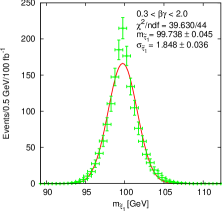
Figure 2: The measured stau mass from the SS with $\sqrt{s}=14$ TeV, $\Delta m=10^{-14}$ GeV, and $L=0.10$ m. The cuts used are mentioned in the text.

In conclusion, sneutrino oscillation is a very important tool to look for lepton number violation at the LHC. However, at the LHC, the sneutrino can be ultrarelativistic, and one should appropriately take into account the Lorentz factor $\gamma\equiv\frac{E}{m}$ and the $L$-dependence while calculating the probability of oscillation. We have seen that the effect is more pronounced when the total decay width of the sneutrino is very small ($\sim 10^{-14}$ GeV), and this can be realized in many different SUSY scenarios. A very interesting signal at the LHC could be two same-sign heavily ionized charged tracks and a soft pion, which can probe a mass splitting all the way down to $\sim 10^{-14}$ GeV with an integrated luminosity as low as 10 ${\rm fb}^{-1}$ for $\sqrt{s}$ = 14 TeV. In fact, for the same mass splitting, it is very evident from Tables I and II that, even for $\sqrt{s}$ = 7 TeV with an integrated luminosity as low as 0.5–1 ${\rm fb}^{-1}$, one would expect to see 4–8 sneutrino oscillation events.

We thank P. Eerola, P. Ghosh, M. Maity, P. Majumdar and B. Mukhopadhyaya for discussions. This work is supported in part by the Academy of Finland (Project No. 115032). D.K.G. acknowledges partial support from the Department of Science and Technology, India, under the grant SR/S2/HEP-12/2006. T.H. thanks the Väisälä Foundation for support.

References

- (1) M. Hirsch, H.V. Klapdor-Kleingrothaus and S.G. Kovalenko, Phys. Lett. B398, 311 (1997).
- (2) Y. Grossman and H.E. Haber, Phys. Rev. Lett. 78, 3438 (1997).
- (3) K. Choi, K. Hwang, and W.Y. Song, Phys. Rev. Lett. 88, 141801 (2002).
- (4) E.J. Chun, Phys. Lett. B525, 114 (2002).
- (5) T. Honkavaara, K. Huitu, and S. Roy, Phys. Rev. D73, 055011 (2006).
- (6) A. Dedes, H.E. Haber, and J. Rosiek, J. High Energy Phys. 11, (2007) 059.
- (7) D.K. Ghosh, T. Honkavaara, K. Huitu, and S. Roy, Phys. Rev. D79, 055005 (2009).
- (8) C.P. Burgess and G.D. Moore, The standard model: A primer (Cambridge University Press, Cambridge, England, 2007), p. 542
- (9) S. Khalil, Phys. Rev. D81, 035002 (2010).
- (10) J.R. Ellis, A.R. Raklev, O.K. Øye, J. High Energy Phys. 10, (2006) 061.
- (11) M. Ibe and R. Kitano, J. High Energy Phys. 08, (2007) 016.