Absolute shifts of Fe I and Fe II lines
in solar active regions (disk center)

Abstract

We estimated absolute shifts of Fe I and Fe II lines from Fourier-transform spectra observed in solar active regions. Weak Fe I lines and all Fe II lines tend to be red-shifted as compared to their positions in quiet areas, while strong Fe I lines, whose cores are formed above the level $\log\tau_{5}\approx-3$ (about 425 km), are relatively blue-shifted, the shift growing with decreasing lower excitation potential. We interpret the results through two-dimensional MHD models, which adequately reproduce red shifts of the lines formed deep in the photosphere. Blue shifts of the lines formed in higher layer do not gain substance from the models.

1 Introduction

We continue the study initiated by us in the papers [5, 6] concerned with the effect of small-scale magnetic fields on solar granulation. The study is based on the observations made by P. Brandt with a Fourier-transform spectrometer (FTS) at the McMath telescope (Kitt Peak National Observatory, USA). The advantages of FTS observations are their high quality and a possibility to observe almost concurrently a large number of lines. Areas close to the solar disk center were observed.

Here we investigate in great depth absolute shifts of Fe I and Fe II lines in low-activity areas (plages) with different integral magnetic fluxes. This is the first time that such an investigation covers a large number of lines formed at various levels in the solar photosphere so that effects of small-scale magnetic fields on height distribution of photospheric velocity field may be studied in detail.

The present state of the investigations on small-scale solar magnetic fields is elucidated in review [22] by Solanki. Determinations of absolute shifts of absorption lines in active areas are not numerous, they are overviewed in [1].

Paper [7] by Brandt and Solanki, similar to [5, 6] and the present paper, is also based on the FTS observations, but only 32 lines were used there to study line parameter variations and 19 lines to determine absolute shifts. Those 19 lines were strong Fe I lines only. The conclusion was made that the lines in active areas had red shifts with respect to their positions in the quiet photosphere. The shifts depend on magnetic field strength (filling factor) and are, on the average, 0.22 pm (about 120 m/s) for lower bisector sections. This result agrees qualitatively with the findings of the studies by Cavallini et al. [8], Livingston [18], Immerschitt and Schroter [16].

At the same time Cavallini et al. [9] dealing with absolute shifts of four lines formed at different photospheric levels obtained a quite different result — shifts of line cores with respect to their positions in the quiet photosphere depend on the region of line core formation: the weak Fe I line at $\lambda$ 614.92 nm displays a red shift, while the strong Ca I line at $\lambda$ 616.22 nm is blue-shifted. A similar result was obtained by Keil et al. [17] for the strong Fe I $\lambda$ 543.45 nm line with a small lower excitation potential (1.01 eV), the core of this line is formed in the upper photospheric layers. Absolute shifts of the line were found to depend on magnetic field polarity, but when the shifts are averaged without regard for local field signs, the line core has a blue shift of about 150 m/s.

Evidence of different behavior of velocity fields with height in the photosphere in active and quiet areas is found also in the analysis of spectral observations with high spatial resolution made by Hanslmeier et al. [14, 15]. If this is the case, lines formed at different levels in the atmosphere should display different absolute shifts.

Thus, the problem needs to be thoroughly investigated on the basis of an extended sample of spectral lines. This is the prime objective of the present study.

2 Observations

The observations used in this study were made in June 1984. The spectral region adequate for reduction extended from $\lambda$ 505 nm to $\lambda$ 665 nm. The theoretical resolution $\lambda$/$\Delta\lambda$ was about 200 000. To assure a sufficient stability of results, the signal integration time during observations was no less than 13.7 min (lifetime of one granule) and the entrance slit was $5^{\prime\prime}\times 25^{\prime\prime}$ (it covered approximately 50 granules). The observations and their comparison to the Liege Atlas data [10] were described in [5, 7]. In all, 23 spectrograms acquired for areas close to the disk center were used in the study.

The magnetic field strength in the areas was estimated by the filling factor $\alpha$ — the relative solar surface area occupied by small-scale magnetic features. The filling factor for the observations used by us was calculated by Solanki [7] from 182 Fe I lines. A simple two-component model was adopted for active areas, it consisted of a “nonmagnetic” quiet photosphere area of size $1-\alpha$ and an area of size $\alpha$ occupied by magnetic elements with a strength of 0.15 T, relative contrast in the continuum was 1.4, and average line weakening was 0.7. The method was described in detail in [7].

Line selection. Lines for the study were selected from two lists. The first list was compiled in [5, 6] especially for studying Fe I and Fe II line asymmetries from the same FTS observations. It comprised 281 lines of Fe I and 30 lines of Fe II between 505 nm and 665 nm. The second list was compiled by Dravins et al. [11, 12] for studying the fine structure of Fe I and Fe II lines in the spectra of the quiet Sun. We used the laboratory wavelengths given in this list. As a result of critical selection we got 189 lines of Fe I and 30 lines of Fe II from the lists [5, 6, 11, 12].

Determination of absolute line shifts involves two problems. First, we have to reduce the FTS wavelengths of solar lines to the absolute scale. Second, we have to choose a way of determining FTS wavelengths from FTS observations.

The first problem was solved by referring to the absolute wavelength scale of photographic solar spectrum derived by Pierce and Breckinridge [20] as well as by using the assumption of Livingston [19] that the absolute shifts of the strong Mg I $\lambda$ 517.27 nm line in active regions coincide with the shifts in quiet regions. The assumption is based on the fact that the Mg I line core is formed high in the atmosphere and its granulation shift is virtually zero, that is, it is virtually independent of small velocity field variations in the lower and middle photosphere. In this case the procedure of reducing FTS wavelengths to the absolute solar wavelength scale [20] is quite simple. First, we found a correction to the absolute scale [20] using the line Mg I $\lambda$ 517.27 nm:

$$\Delta_{abs}=\lambda_{FTS}^{MgI}-\lambda_{P\&B}^{MgI},$$

where $\lambda_{FTS}^{MgI}$ is the FTS wavelength of the Mg I line, $\lambda_{P\&B}^{MgI}$ is the wavelength of the same line in the absolute scale of Pierce and Breckinridge [20]. Then we reduced line wavelengths measured from the FTS spectra ($\lambda_{FTS}$) to the absolute scale:

$$\lambda_{abs}^{FTS}=\lambda_{FTS}-\Delta_{abs}.$$

Thus the correction of the FTS wavelengths was made for tne effects of the relative motion of the Sun and the Earth as well as for possible systematic scale shifts.

Now we turn to the second problem — the determination of line wavelengths from FTS observations, $\lambda_{FTS}$. Since the wavelengths $\lambda_{FTS}$ are referred to the absolute scale of tables [20], they must be determined in the same way as in [20]. The wavelengths in [20] were measured on photographic plates by an operator with a special measuring machine. After a series of numerical experiments and taking into consideration the results of Dravins et al. [12], we concluded that the most stable results could be obtained when $\lambda_{FTS}$ was found as a weighted mean wavelength of line core (or center of gravity of line core). The line core was defined as one-tenth of the line profile measured from the minimum profile point. To upgrade the estimate accuracy, we interpolated the original observations by a weighted parabola with a 0.2 pm step.

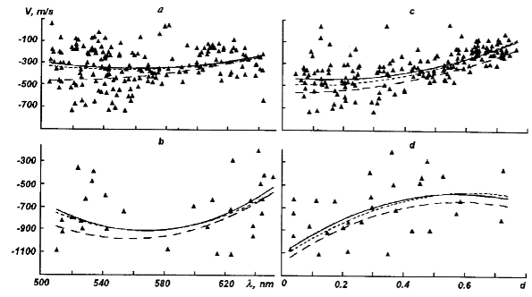
Figure 1: Absolute line shifts derived from nine FTS spectra for the quiet photosphere in this study and from tables [11, 12]. Shown is only our sample of Fe I and Fe II lines. Solid lines and triangles) results from [11, 12]. Long dashes) shifts with respect to the Mg I $\lambda$ 517.27 nm line derived in this study, average over all lines; short dashes) shifts with respect to 12 reference Fe I lines, a and b) shifts of Fe I and Fe II lines depending on wavelength, c and d) shifts depending on central line depth.

Radial velocities were determined by the well-known expression which relates line shifts to velocities:

$$V_{R}=c\cdot(\lambda_{abs}-\lambda_{lab})/\lambda_{lab}-2.12\cdot 10^{-6}\cdot c,$$

$\lambda_{lab}$ being laboratory wavelengths [11, 12]. To assess variations in the FTS dispersion, we compared the average radial velocities derived from nine FTS spectra of quiet areas with the data from [11, 12]. Recall that solar line wavelengths in [11, 12] were also taken from tables [20]. The wavelength dependence of radial velocities (Fig. 1) suggests that the FTS observations require a correction for dispersion variations. The correction was made with the use of lines with small granulation shifts between their positions in the active and quiet photosphere. After preliminary calculations we selected such lines distributed over the whole wavelength range observed. An analysis revealed that the smallest differences in absolute shifts between quiet and active regions occurred in two groups of moderately strong Fe I lines. One group included lines with lower excitation potentials $EPL$ from 2 to 3.5 eV, equivalent widths $W$ from 7.7 to 10 pm, and central depths $d$ from 0.65 to 0.79; the lines in the other group have $EPL>3.5$ eV, $W=10.0$–12.0 pm, $d=0.70$–0.79. Using specially calculated [21] sensitivity indicators (coefficients that characterize line sensitivity to variations in particular parameters of the medium), we excluded the temperature-sensitive lines from the list of selected lines (28 out of 189). The final list of 12 reference Fe I lines is given in Table 1.

Table 1: Spectral lines selected for referring the FTS wavelength scale to the absolute scale of solar wavelengths by Pierce and Breckinridge [20]

$\lambda$, nm (laboratory) [11, 12]	$\lambda$, nm (solar) [20]	$EPL$, eV	$d_{obs}$	$W_{obs}$, pm	$\log\tau_{5D}$
509.07750	509.07807	4.26	0.752	10.04	-2.41
514.17387	514.17460	2.42	0.768	9.80	-2.76
519.87114	519.87171	2.22	0.792	9.96	-3.05
525.06447	525.06527	2.20	0.793	10.35	-3.09
536.48717	536.48801	4.44	0.785	13.18	-2.99
538.94786	538.94866	4.41	0.719	9.57	-2.36
546.29601	546.29672	4.47	0.735	9.70	-2.70
548.77433	548.77512	4.14	0.722	12.02	-3.00
557.60874	557.60970	3.43	0.772	12.30	-3.06
566.25153	566.25233	4.18	0.719	11.16	-3.10
624.63172	624.63271	3.60	0.716	12.37	-3.02
641.16468	641.16586	3.65	0.717	14.32	-3.13

These lines are of low sensitivity to temperature (it is the same for all lines — $(\delta d/d)/(\delta T/T)=-1.5$), their central depths range from 0.72 to 0.79, and equivalent widths range from 10 to 14 pm. The lines were used to find dispersion corrections for every spectrum:

$$\Delta_{dis}(\lambda)=\lambda_{abs}^{FeI}-\lambda_{P\&B}^{FeI}.$$

Then the dispersion curve coefficients $a$ and $b$ were found by linear approximation:

$$\Delta_{dis}(\lambda)=a+b\lambda,$$

and dispersion corrections were introduced to every FTS wavelength of the other lines:

$$\lambda_{abs}=\lambda_{abs}^{FTS}-(a+b\lambda).$$

The radial velocities calculated with respect to 12 reference Fe I lines showed a much better agreement with the data by Dravins et al. [11, 12] (Fig. 1). When 12 reference Fe I lines are used, the Mg I line can be eliminated from the calculations. However, we determined the radial velocities relative to the magnesium line as well, since the change in dispersion is not very large in our case and reference lines are not ideal for correcting it.

3 Results

The absolute shifts obtained by us and averaged over nine spectra are compared in Fig. 1 with the shifts derived in [11, 12]. The average cosine of the angle of radiation direction with the external normal to the area surface, $\mu$, is 0.988 for all nine areas observed. Our results are obviously different from those of [11, 12]. The discordance is different for moderate, strong, and weak lines. We believe that the discordance is due mainly to the procedures used for determining line wavelengths and to the fact that the spectral resolution was different in our observations and those in [11, 12]. Nevertheless, for the radial velocities derived with respect to the reference Fe I lines the discordance (about 50 m/s on the average) may be reckoned as small compared to the scatter in the data. Qualitatively the discordance is independent of the excitation potential and ionization stage, except for strong lines with $EPL>3.5$ eV, most reference lines falling in this category. The lines in this group show, of course, better agreements with [11, 12].

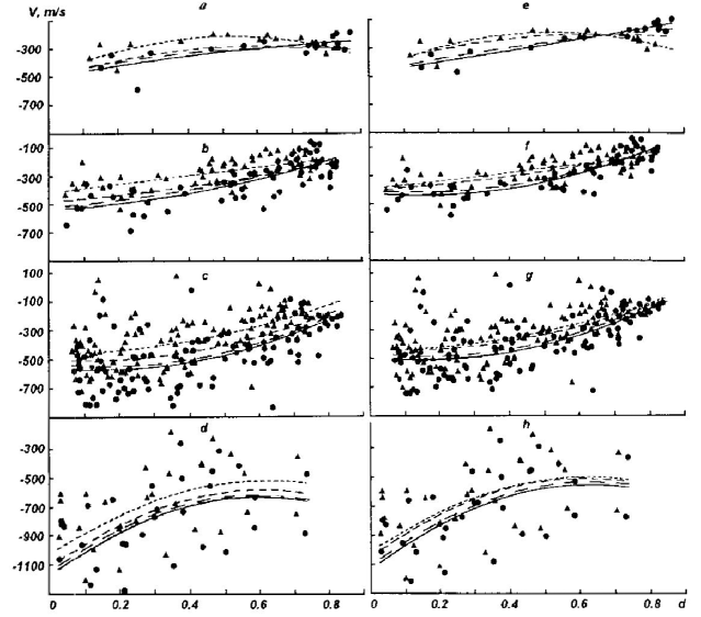
Figure 2: Average absolute line shifts with respect to the Mg I $\lambda$ 517.27 nm line (a–d) and 12 Fe I lines (e–h) as functions of central line depth. Central depths were determined relative to the local continuum for each spectrum. a,e) Fe I lines with $EPL<2$ eV; b,f) $EPL=2$–3.5 eV; c,g) $EPL>3.5$ eV; d,h) Fe II lines. Solid lines and dots) data from nine spectra with $\alpha\approx 0$%, long dashes) from six spectra with $\alpha\approx 3$ %, short dashes) from six spectra with $\alpha\approx 8$%, triangles and dotted line) from two spectra with $\alpha\approx 11$%.

Figures 2 a–d display the shifts relative to the magnesium line, and Figs 2 e–h show the shifts relative to 12 reference Fe I lines. We divided 23 FTS spectra into four groups depending on filling factor $\alpha$: group 1 — nine spectra, $\overline{\alpha}=0.3$% $\approx$ 0%, $\overline{\mu}=0.988$; group 2 – six spectra, $\overline{\alpha}=$2.5% $\approx$ 3%, $\overline{\mu}=0.962$; group 3 – six spectra, $\overline{\alpha}=7.5$% $\approx$ 8%, $\overline{\mu}=0.953$; group 4 – two spectra, $\overline{\alpha}=11.4$% $\approx$ 11%, $\overline{\mu}=0.955$. The Fe I lines were divided into three groups in accordance with their $EPL$: less than 2 eV, 2–3.5 eV, and more than 3.5 eV. The dependence of absolute shifts on $\alpha$, $EPL$, line strength, and ionization stage is apparent. First of all we note that all Fe II lines in active areas are red-shifted as compared to quiet areas, the shift growing with $\alpha$. This inference is unaffected by the choice of reference lines. The largest relative red shifts are observed in the spectra with $\alpha\approx 11$ per cent, they are about 100 m/s when the dispersion is corrected and about 160 m/s when determined relative to the magnesium line only without dispersion correction.

As to the Fe I lines, the results heavily depend on $EPL$ and line strength. The lines with $EPL>3.5$ eV behave similarly to the Fe II lines: the shifts of most lines are more red in active areas as compared to the quiet photosphere. This inference is also unaffected by the choice of reference lines. At the same time strong lines in active areas demonstrate absolute shifts close to those observed in the quiet photosphere, this result being the same when calculations are made with the magnesium line or with 12 reference Fe I lines. The tendency is stronger for lines with smaller excitation potentials: the strong lines either display shifts close to those in the quiet photosphere or have more violet shifts in magnetic areas. When the change in dispersion is allowed for, the largest violet shifts are observed in the areas with $\alpha$ = 11 per cent, they are about 180 m/s for strong Fe I lines with $EPL<2$ eV and about 80 m/s for lines with $EPL=2$–3.5 eV. The largest red shift is virtually the same (120 m/s) for all groups of weak and moderate Fe I lines.

It should be stressed that the variations of absolute shifts in active areas with respect to their positions in quiet photosphere areas are small and lie within confidence limits for the corresponding mean values, and so we may speak about tendencies only. Nevertheless, it is of interest that our results point to the change of sign in absolute shifts of Fe I lines in active areas with respect to the quiet photosphere if the line cores are formed above the level $\log\tau_{5}~{}\approx~{}-3$, i.e., above 425 km. It is pertinent to note that the absolute shifts calculated relative to the magnesium line or strong iron lines demonstrate the same trends. This fact substantiates the reality of the results obtained.

We have already noted that in the early study [7] based on the same FTS observations Brandt and Solanki inferred that 19 strong Fe I lines had, on the average, larger red shifts in active areas. The list of those lines included seven lines with $EPL>3.5$ eV, nine lines with $EPL=2$–3.5 eV, and three lines with $EPL<2$ eV. To find out why the data from [7] disagreed with our results, we repeated the calculations made in [7], allowing for the absolute line shifts derived in this study. Recall that absolute shifts of bisectors of individual lines were dealt with in [7], and then their averaging was done. When treated in such a manner, the average bisectors were found to have red shifts in their wings and at the intermediate level in active areas with respect to the quiet photosphere. At the same time, the positions of individual bisectors of the lines studied had a strong scatter near line cores at an intensity level of about 0.2, this scatter being due to the wide range of $EPL$ in this line group. That is why the authors of [7] left the lower bisector part out of consideration, as seen from Fig. 13 in [7], and formulated their conclusion which did not characterize the behavior of line cores. We believe, therefore, that our results are not in variance with the results of [7], since they describe the behavior of absolute line shifts at various levels of residual line intensities: the shifts investigated in [7] refer to the levels from line wings to a residual intensity of 0.4, while the shifts of line cores only are dealt with in this study.

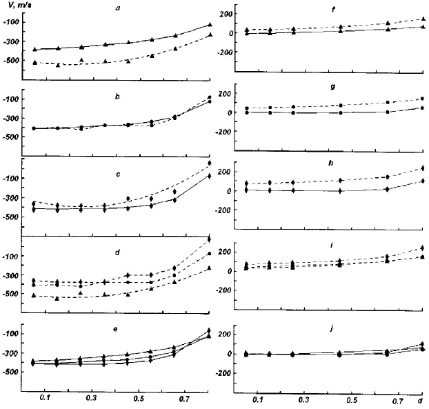
Figure 3: Absolute shifts of the artificial Fe I lines $\lambda$ 500 nm calculated with 2-D MHD models [6] (a-e) and [2, 3] (f-j) as functions of central line depth. Central depths of lines from nonmagnetic HD models are given. Solid lines) 2-D nonmagnetic HD model calculations, dashed lines) 2-D MHD model synthesis; triangles, a,f) lines with $EPL=0$ eV; dots, b,g), lines with $EPL=2.5$ eV; diamonds, c,h) lines with $EPL=5$ eV; d,i) lines calculated with MHD models only; e,j) lines calculated with nonmagnetic HD models only.

As $\overline{\mu}$ can be somewhat different for the groups of spectra, the limb effect might show up in our results [4]. To examine this problem, we selected three spectra for areas lying at the same distance from the disk center $\mu=0.97$ but having various $\alpha$ – 0.006, 0.026, and 0.114. The spectra were acquired on the same day in the course of 34 min. The results obtained from these spectra were found to be in qualitative agreement with those obtained from 23 spectra. Thus, a possible limb effect does not change noticeably our final results derived from the spectra used.

4 Interpretation of the results

Earlier, Cavallini et al. [9] proposed their interpretation of the line shifts in solar spectra. They suggested that the penetrating photos pheric convection becomes less efficient in the presence of small-scale magnetic fields. In this case horizontal magnetic lines of force prevent ascending flows from penetrating in the middle and upper photosphere while the velocities grow in descending flows around magnetic tubes. Thus, for the lines formed deep in the photosphere the violet convective shift decreases above granules and the red shift increases above intergranular lanes — the line as a whole acquires a redder absolute shift as compared to the quiet photosphere. In the lines that form in the upper layers the contribution to the red shift from the regions above descending flows is smaller, since the penetrating convection is somewhat “submerged” in active areas.

Hanslmeier et al. [14] found from spectra with high spatial resolution that a strong line formed in a magnetic region in the upper layers may have a redder shift above a granule than above intergranular lanes. In other words, inversion may occur in the motions in the upper photosphere. At the same time, a line formed in deeper layers in the same area displays the usual pattern: its shift is violet above granules and red above porules.

Our quantitative interpretation is based on two sets of theoretical self-consistent two-dimensional MHD models. The models and some results of their application to spectral observations are described in [2, 3, 6]. Three sets of models with mean magnetic fluxes of 10, 20, and 30 mT were presented in papers [2, 3].

Table 2: Basic parameters of the 2-D MHD models used

Model parameter	Atroshchenko & Sheminova [6]	Brandt & Gadun [2]
Area size ($x,~{}z$), km	2520$\times$2030	3840$\times$1920
Grid dimension, Step on $x,~{}z$	72$\times$58, 35 km	$256\times 128$, 15 km
Model atmosphere layers (above $\tau$=1)	900 km	600 km
Radiation transfer	2D momentum method,	2D momentum method,
	variable Eddington factors	variable Eddington factors
Absorption coefficient	monochromatic, 97 frequencies,	Rosseland coefficient,
in photospheric layers	absorption taken into	selective absorption corrected
	account directly (ODF)	in four frequency intervals
Side boundary conditions	symmetric impenetrability	periodic
Upper boundary conditions	free	free
Lower boundary conditions	free	closed
Mean magnetic field strength in the model	45 mT	30 mT
Magnetic field strength maximum	300 mT	200 mT
at the level $\tau$ = 1 in a magnetic tube
Largest Wilson depression in a tube	$\approx$300 km	$\approx$200 km
Magnetic tube width at $\tau$ = 1	$\approx$300 km	$\approx$250 km

We used the model with the largest flux. Table 2 gives the most important model parameters.

We calculated the sets of artificial Fe I and Fe II lines with the wavelength $\lambda$ 500 nm and excitation potentials of 0, 2.5, 5 eV (Fe I) and 2, 3.5, 6 eV (Fe II). The LTE line profiles of these lines were calculated with the SPANSAT code [13]. First we took the corresponding two-dimensional inhomogeneous hydrodynamic models calculated with the same approximations as in MHD models but without magnetic fields and found such values of $Agf$ (the product of abundance by oscillator strength) that fixed central line depths might be obtained: 0.05, 0.15, …, 0.65, 0.8 for Fe I and 0.05, 0.15, …, 0.65 for Fe II. Then these values of $Agf$ were used to calculate lines with 2-D MHD models in the LTE approximation without broadening by magnetic fields. Figures 3 and 4 show the absolute shifts thus obtained for Fe I and Fe II lines, respectively.

First of all we call attention to the fact that models [2, 3] have overheated atmospheres because the absorption by spectral lines was overestimated in them, and this results in a smaller vertical velocity gradient. That is why the lines calculated with 2-D HD models [2, 3] have underestimated violet shifts.

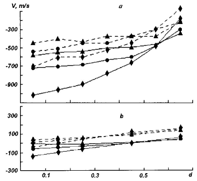
Figure 4: Absolute shifts of the artificial Fe II lines $\lambda$ 500 nm calculated with 2-D MHD models [6] (a) and [2, 3] (b). Solid lines) calculations with 2-D nonmagnetic HD models, dashed lines) 2-D MHD model synthesis, triangles) lines with $EPL=2$ eV, dots) $EPL=3.5$ eV, diamonds) $EPL=6$ eV.

The absolute line shifts are qualitatively the same in both sets of nonmagnetic HD models (Figs 3e and 3j). The shifts of moderate-strong lines depend on $EPL$ – the violet shift is larger the higher the excitation potential (i.e., the relative contribution from ascending flows is greater for deep-formed lines). The models for strong Fe I lines reproduce the well-known effect — lines with high $EPL$ display redder shifts due to an inverse distribution of temperature variations in the middle and upper photosphere. These patterns are in good qualitative agreement with observations [12].

The 2-D MHD models demonstrate the reverse dependence of line shifts on $EPL$ (Figs 3d and 3i: the shifts become redder with growing $EPL$, reflecting the growing role of descending flows in the lower layers. However, the shifts of Fe I lines from MHD models relative to the corresponding nonmagnetic HD models (this corresponds to an observational comparison between active areas and quiet photosphere areas) are represented in different ways by two sets of MHD models. Models [2, 3] show a slightly growing relative red shift (up to 100 m/s) between HD and MHD models when $EPL$ increases. The other set of MHD models [6] show a more intricate pattern: the lines with $EPL=0$ are violet-shifted, the shift is almost the same for all lines; the shifts of the Fe I lines with $EPL=2.5$ eV found from MHD models equal the shifts from nonmagnetic HD models; and the lines with high excitation potentials (5 eV) have red shifts.

There are no substantial discrepancies between the models for Fe II lines (Fig. 4). In both model sets the MHD model lines are red-shifted with respect to nonmagnetic HD models.

So, we may state that two-dimensional MHD models [2, 3, 6] reproduce qualitatively alike the red shifts of the lines formed deep in the photosphere. The shifts are due to growing areas of descending flows, where bundles of magnetic lines of force are located, and to growing velocities of descending flows. However, there is essential discordance between the models when lines formed in the middle and upper photosphere are considered. The discordance owes its existence to some drawbacks of both model sets. Models [6] have a very rough spatial step – 35 km, and this could distort the temperature distribution in the middle and upper photosphere when a developed magnetic configuration was calculated. Models [2, 3] overestimate the heating of atmospheric layers due to an overestimated absorption in line frequencies, and this also may distort the velocity field. Thus, the violet shifts found by Cavallini et al. [9] and in our study for the lines that form in the upper layers are not confirmed within the scope of the 2-D MHD models used by us, although these models need serious improvements.

5 Conclusion

FTS observations were used to estimate possible absolute shifts of Fe I and Fe II lines in active regions. We conclude that weak Fe I lines and all Fe II lines are likely to be red-shifted with respect to their positions in the quiet photosphere, while strong Fe I lines with low $EPL$s, their cores being formed above the level $\log\tau_{5}\approx-3$ ($\approx$425 km), have more violet shifts.

The results were interpreted on the basis of 2-D MHD models that reproduce quite adequately the red shifts of the lines formed deep in the photosphere, but violet shifts of the lines formed in the upper photospheric layers are not confirmed within the scope of these models.

Acknowledgements. We wish to thank the National Optical Astronomical Observatory/National Solar Observatory (Tucson, Arizona, USA) and especially J. Brault and B. Graves for support in the FTS observations; S. Solanki for filling factor calculations; R. Rutten for assistance in the organization of this investigation. The study was partially financed by the Joint Foundation of the Government of Ukraine and International Science Foundation (Grant No. K11100).

References

- [1] I. N. Atroshchenko, A. S. Gadun, and R. I. Kostyk, ”Fine structure of Fraunhofer lines: Observation results and interpretation,” Kinematika i Fizika Nebes. Tel [Kinematics and Physics of Celestial Bodies], vol. 6, no. 6,pp. 3-20, 1990.
- [2] I. N. Atroshchenko and V. A. Sheminova, ”Numerical simulation of the interaction between solar granules and small-scale magnetic fields,” Kinematika i Fizika Nebes. Tel [Kinematics and Physics of Celestial Bodies], vol. 12, no. 4, pp. 32-45, 1996.
- [3] I. N. Atroshchenko and V. A. Sheminova, ”Simulation of spectral effects with the use of 2-D MHD models of the solar photosphere,” Kinematika i Fizika Nebes. Tel [Kinematics and Physics of Celestial Bodies], vol. 12, no. 5, pp. 32-47, 1996.
- [4] H. Balthasar, ”Asymmetries and wavelengths of solar spectral lines and the solar rotation determined from Fourier-transform spectra,” Solar Phys., vol. 93, no. 2, pp. 219-241, 1984.
- [5] P. N. Brandt and A. S. Gadun, ”Changes in the parameters of Fe I spectral lines as a function of the magnetic flux (solar disk center),” Kinematika i Fizika Nebes. Tel [Kinematics and Physics of Celestial Bodies], vol. 9, no. 3, pp. 8-22, 1993.
- [6] P. N. Brandt and A. S. Gadun, ”Changes in the Fe II line parameters depending on magnetic flux (solar disk center),” Kinematika i Fizika Nebes. Tel [Kinematics and Physics of Celestial Bodies], vol. 11, no. 4, pp. 44-59, 1995.
- [7] P. N. Brandt and S. K. Solanki, ”Solar line asymmetries and the magnetic filling factor,” Astron. and Astrophys., vol. 231, no. 1, pp. 221-234, 1990.
- [8] F. Cavallini, G. Ceppatelli, and A. Righini, ”Asymmetry and shift of three Fe I photospheric lines in solar active regions,” Astron. and Astrophys., vol. 143, no. 1, pp. 116-121, 1985.
- [9] F. Cavallini, G. Ceppatelli, and A. Righini, ”Profile variations of some photospheric lines as observed in active regions across the solar disk,” Astron. and Astrophys., vol. 205, no. 1/2, pp. 278-288, 1988.
- [10] L. Delbouille, L. Neven, and G. Roland, Photometric Atlas of the Solar Spectrum from 3000 to 10000, Institut d’Astrophysique, Liege, 1973.
- [11] D. Dravins, B. Larsson, and A. Nordlund, ”Solar Fe II line asymmetries and wavelength shifts,” Astron. and Astrophys., vol. 158, no. 1/2, pp. 83-88, 1986.
- [12] D. Dravins, L. Lindegren, and A. Nordlund, ”Solar granulation: influence of convection on spectral line asymmetries and wavelength shifts,” Astron. and Astrophys., vol. 96, no. 1/2, pp. 345-364, 1981.
- [13] A. S. Gadun, V. A. Sheminova. SPANSAT: Program for Calculating the LTE Absorption Line Profiles in Stellar Atmospheres, Kyiv, 1988, Inst. Theor. Phys., Academy of Sciences of UkrSSR, Preprint No. ITF-88-87P.
- [14] A. Hanslmeier, W. Mattig, and A. Nesis, ”High spatial resolution solar photospheric line observations in Ca+ active regions,” Astron. and Astrophys., vol. 244, no. 2, pp. 521-532, 1991.
- [15] A. Hanslmeier, A. Nesis, and W. Mattig, ”The variation of the solar granulation structure in active and non-active regions,” Astron. and Astrophys., vol. 251, no. 1, pp. 307-311, 1991.
- [16] S. Immerschitt and E. H. Schroter, ”The behaviour of asymmetry and other profile parameters of the Fe I 5576.1 Åline in solar regions of varying magnetic activity,” Astron. and Astrophys., vol. 208, no. 1/2, pp. 307-313, 1989.
- [17] S. L. Keil, Th. Roudier, E. Cambell, et al., ”Observation and interpretation of photospheric line asymmetry changes near active regions,” in: Solar and Stellar Granulation, R. J. Rutten and G. Severino (Editors), pp. 273-281, Kluwer, Dordrecht, 1989.
- [18] W. C. Livingston, ”Magnetic fields, convection and solar luminosity variability,” Nature, vol. 297, no. 5863, pp. 208-209, 1982.
- [19] W. C. Livingston, ”Magnetic fields and convection: new observations,” in: Solar and Stellar Magnetic Fields: Origin and Coronal Effects, IAU Symp. No. 102, pp. 149-153, Reidel, Dordrecht, 1983.
- [20] A. K. Pierce and J. B. Breckinridge, The Kitt Peak Table of Photographic Solar Spectrum Wavelengths, Kitt Peak Nat. Obs., Tucson, 1973 (Contribution No. 559).
- [21] V. A. Sheminova, ”The parameters of sensitivity of Fraunhofer lines to the temperature gas pressure and microturbulent velocity,” Kinematika i Fizika Nebes. Tel [Kinematics and Physics of Celestial Bodies], vol.9, no. 5, pp. 27-43, 1993.
- [22] S. K. Solanki, ”Small-scale solar magnetic fields: an overview,” Space Sci Rev., vol. 63, pp. 1-188, 1993.