Coherent excitation-energy transfer and quantum entanglement in a dimer

Abstract

We study coherent energy transfer of a single excitation and quantum entanglement in a dimer, which consists of a donor and an acceptor modeled by two two-level systems. Between the donor and the acceptor, there exists a dipole-dipole interaction, which provides the physical mechanism for coherent energy transfer and entanglement generation. The donor and the acceptor couple to two independent heat baths with diagonal couplings that do not dissipate the energy of the non-coupling dimer. Special attention is paid to the effect on single-excitation energy transfer and entanglement generation of the energy detuning between the donor and the acceptor and the temperatures of the two heat baths. It is found that, the probability for single-excitation energy transfer largely depends on the energy detuning in the low temperature limit. Concretely, the positive and negative energy detunings can increase and decrease the probability at steady state, respectively. In the high temperature limit, however, the effect of the energy detuning on the probability is negligibly small. We also find that the probability is negligibly dependent on the bath temperature difference of the two heat baths. In addition, it is found that quantum entanglement can be generated in the process of coherent energy transfer. As the bath temperature increases, the generated steady-state entanglement decreases. For a given bath temperature, the steady-state entanglement decreases with the increase of the absolute value of the energy detuning.

I Introduction

Coherent excitation energy transfer is an important step of photosynthesis Blankenship , in which photosynthetic pigments capture the solar light to create electronic excitations and then transfer the excitation energy to a reaction center May-Kuhn ; Fleming1994 ; Fleming2009 ; Renger2009 ; Fleming2007 ; Flemingnature . Usually, the transfer of a single excitation from the pigment where the electronic excitation is created to the reaction center is a very complicated physical process, since the practical transfer process takes place on a complicated network of pigments. However, the basic physical mechanism can be revealed in such a light-harvesting complex by studying a basic part: a dimer system which consists of a donor and an acceptor modeled by two two-level systems.

On a complicated network of pigments, there generally exist two kinds of interactions. On one hand, between any two pigments there exists a dipole-dipole interaction, which results in excitation energy transfer. On the other hand, the pigments interact inevitably with their surrounding environments such as the nuclear degrees of freedom and the proteins. Corresponding to different cases for the scale of the two kind of interactions, different approaches have been proposed to study the single-excitation energy transfer. Concretely, when the dipole-dipole interactions between any two pigments are much weaker than the interactions of the pigments with their environments, the energy transfer process can be well characterized by the Förster theory Forster1948 , in which the evolution of the network is calculated perturbatively up to the second order in the dipole-dipole interactions between the pigments; When the interactions of the pigments with their environments are much weaker than the dipole-dipole interactions between any two pigments, various approaches based on the quantum master equation have been proposed (e.g., Refs. Ishizaki2009 ; Jang2008 ; Palmieri2009 ; Aspuru-Guzik2008 ; Aspuru-Guzik20091 ; Aspuru-Guzik20092 ; Aspuru-Guzik20093 ; Plenio2008 ; Plenio20091 ; Castro2008 ; Castro2009 ; Nazir2009 ; Nori2009 ; Liang2010 ; Yang2010 ), in which the evolution of the network is calculated perturbatively up to the second order in the interactions between the pigments and their environments.

With the above considerations, in this article we study single-excitation energy transfer in a dimer, which consists of a donor and an acceptor modeled by two two-level systems. Obviously, when the donor and the acceptor are decoupled, it is impossible to realize energy transfer between them. Therefore, the simplest way to realize energy transfer is to turn on a non-trivial interaction (for example, the dipole-dipole interaction) between the donor and the acceptor. Then a single excitation can coherently oscillate between the donor and the acceptor. However, in this case, there is no steady-state energy transfer, namely the transferred energy can not approach to a stationary value. In the presence of environments, the donor and the acceptor will inevitably couple with environments. In general, the coupling form between the donor (acceptor) and its environment is diagonal in the representation of the free Hamiltonian of the donor (acceptor). Physically, due to this type of coupling, although the excitation energy will not decay into the environments, it will induce a steady-state energy transfer between the donor and the acceptor. Since in practical cases both the characteristic frequency and the heat bath temperatures of the donor and the acceptor may be different due to different chemical structures, we study in detail how the characteristic frequencies and the heat bath temperatures of the donor and acceptor affect the efficiency of the excitation energy transfer. This is one point of the motivations of our present work.

In the presence of the interactions between the pigments for transferring energy, a naturally arising question is how about the quantum entanglement among the pigments which are involved in the energy transfer process. Because quantum entanglement is at the heart of the foundation of quantum mechanics Bell1987 ; Einstein1935 and quantum information science (e.g., Refs. Nielsen2000 ; Qian2005 ), it is interesting to know how is the dynamics of the created quantum entanglement in the dimer system during the process of single-excitation energy transfer. This is the other point of the motivations of our present investigations. In fact, recently people have become aware of quantum entanglement in some chemical and biologic systems (e.g., Refs. Briegel2008 ; Briegel2009 ; Plenio20091 ; Thorwart2009 ; Sarovar2009 ; Caruso2009 ) such as photosynthetic light-harvesting complexes Plenio20091 ; Sarovar2009 ; Caruso2009 .

This article is organized as follows: In Sec. II, we present the physical model and the Hamiltonian for studying the single-excitation energy transfer. A dimer consists of a donor and an acceptor, which are immersed in two independent heat baths. Between the donor and the acceptor, there exists a dipole-dipole interaction, which provides the physical mechanism for coherent excitation energy transfer and entanglement generation. In Sec. III, we derive a quantum master equation to describe the evolution of the dimer. Based on the quantum master equation we obtain optical Bloch equations and their solutions. In Sec. IV, we study single-excitation energy transfer from the donor to the acceptor. The effect on the transfer probability of the energy detuning and the bath temperatures are studied carefully. In Sec. V, we study the quantum entanglement between the donor and the acceptor by calculating the concurrence. We conclude this work with some remarks in Sec. VI. Finally, we give an appendix for derivation of quantum master equation (7).

II Physical model and Hamiltonian

As illustrated in Fig. 1(a), the physical system under our consideration is a dimer, which consists of a donor and an acceptor modeled by two two-level systems (TLSs), TLS$1$ (donor) and TLS$2$ (acceptor), with respective energy separations $\omega_{1}$ and $\omega_{2}$. The donor and the acceptor are immersed in two independent heat baths of temperatures $T_{1}$ and $T_{2}$, respectively. Between the donor and the acceptor there exists a dipole-dipole interaction of strength $\xi$.

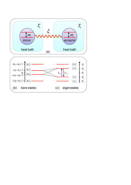
Figure 1: (Color online) (a) Schematic of the physical system. A donor and an acceptor are immersed in two independent heat baths of temperatures $T_{1}$ and $T_{2}$, respectively. A dipole-dipole interaction of strength $\xi$ exists between the donor and the acceptor, which are described by two two-level systems with resonant frequencies $\omega_{1}$ and $\omega_{2}$, respectively. (b) The energy levels of the bare states $|\eta_{n}\rangle$ ($n=1,2,3,4$) of the donor and the acceptor when they are decoupling. (c) The energy levels of the eigenstates $|\lambda_{n}\rangle$ ($n=1,2,3,4$) of the coupled donor and acceptor. The corresponding eigen-energies are denoted by $E_{n}$. The parameters $\Gamma_{23}$ and $\Gamma_{32}$ are, respectively, the bath induced transition rates from states $|\lambda_{2}\rangle$ to $|\lambda_{3}\rangle$ and from states $|\lambda_{3}\rangle$ to $|\lambda_{2}\rangle$.

The Hamiltonian of the total system, including the two coupled TLSs and their heat baths, is composed of three parts,

$$H=H_{\textrm{TLSs}}+H_{B}+H_{I},$$ (1)

where $H_{\textrm{TLSs}}$ is the Hamiltonian (with $\hbar=1$) of the two coupled TLSs,

$$H_{\textrm{TLSs}}=\frac{\omega_{1}}{2}\sigma_{1}^{z}+\frac{\omega_{2}}{2}\sigma_{2}^{z}+\xi\left(\sigma_{1}^{+}\sigma_{2}^{-}+\sigma_{1}^{-}\sigma_{2}^{+}\right).$$ (2)

Concretely, the first two terms in Eq. (2) are free Hamiltonians of the two TLSs, which are described by the usual Pauli operators $\sigma_{l}^{+}=(\sigma_{l}^{-})^{{\dagger}}=(\sigma_{x}+i\sigma_{y})/2=\left|e\right\rangle_{ll}\left\langle g\right|$ and $\sigma_{l}^{z}=\left|e\right\rangle_{ll}\left\langle e\right|-\left|g\right\rangle_{ll}\left\langle g\right|$, where $|g\rangle_{l}$ and $|e\rangle_{l}$ are, respectively, the ground and excited states of the $l$th ($l=1,2$) TLS, namely TLS$l$. The last term in Eq. (2) depicts the dipole-dipole interaction of strength $\xi$ between the two TLSs. This dipole-dipole interaction provides the physical mechanism for excitation energy transfer and entanglement generation between the two TLSs.

The Hilbert space of the donor and the acceptor is of four dimension with the four basis states $|\eta_{1}\rangle=|ee\rangle$, $|\eta_{2}\rangle=|eg\rangle$, $|\eta_{3}\rangle=|ge\rangle$, and $|\eta_{4}\rangle=|gg\rangle$, as shown in Fig. 1(b). In the presence of the dipole-dipole interaction, a stationary single-excitation state should be delocalized and composed of a combination of the single-excitation in the two TLSs. According to Hamiltonian (2), we can obtain the following four eigenstates

$$\left|\lambda_{1}\right\rangle = \left|ee\right\rangle,$$

$$\left|\lambda_{2}\right\rangle = \cos\left(\theta/2\right)\left|eg\right\rangle+\sin\left(\theta/2\right)\left|ge\right\rangle,$$

$$\left|\lambda_{3}\right\rangle = -\sin\left(\theta/2\right)\left|eg\right\rangle+\cos\left(\theta/2\right)\left|ge\right\rangle,$$

$$\left|\lambda_{4}\right\rangle = \left|gg\right\rangle,$$ (3)

and the corresponding eigenenergies $E_{1}=-E_{4}=(\omega_{1}+\omega_{2})/2$ and $E_{2}=-E_{3}=\sqrt{\Delta\omega^{2}/4+\xi^{2}}$, as shown in Fig. 1(c), by solving the eigen-equation $H_{\textrm{TLSs}}\left|\lambda_{n}\right\rangle=E_{n}\left|\lambda_{n}\right\rangle$ ($n=1,2,3,4$). Here we introduce the energy detuning $\Delta\omega=\omega_{1}-\omega_{2}$ and the mixing angle $\theta$ defined by $\tan\theta=2\xi/\Delta\omega$. Note that here the mixing angle $0<\theta<\pi$. Therefore, when $\Delta\omega>0$, namely $\omega_{1}>\omega_{2}$, we have $\theta=\arctan(2\xi/\Delta\omega)$; however, when $\Delta\omega<0$, that is $\omega_{1}<\omega_{2}$, we have $\theta=\arctan(2\xi/\Delta\omega)+\pi$.

As pointed out by Caldeira and Leggett Leggettnp , when the couplings of a system with its environment are weak, it is universal to model the environment of the system as a harmonic oscillator heat bath. In this work, we suppose that the couplings of the TLSs with their environments are weak, then it is reasonable to model the environments as two harmonic oscillator heat baths with the Hamiltonian

$$H_{B} = H^{(a)}_{B}+H^{(b)}_{B}.$$ (4)

Here $H^{(a)}_{B}$ and $H^{(b)}_{B}$ are respectively the Hamiltonians of the heat baths for the TLS$1$ and TLS$2$,

$$H^{(a)}_{B} = \sum_{j}\omega_{aj}a_{j}^{\dagger}a_{j},\hskip 14.22636ptH^{(b)}_{B}=\sum_{k}\omega_{bk}b_{k}^{\dagger}b_{k},$$ (5)

where $a^{{\dagger}}_{j}$ ($b^{{\dagger}}_{k}$) and $a_{j}$ ($b_{k}$) are, respectively, the creation and annihilation operators of the $j$th ($k$th) harmonic oscillator with frequency $\omega_{aj}$ ($\omega_{bk}$) of the heat bath for TLS$1$ (TLS$2$). In practical systems of excitation energy transfer, the environment is composed of the nuclear degrees of freedom of the molecules.

The interaction Hamiltonian of the TLSs with their heat baths reads (e.g., Refs. Ishizaki2009 ; Jang2008 ; Palmieri2009 ; Aspuru-Guzik2008 ; Aspuru-Guzik20091 ; Aspuru-Guzik20092 ; Aspuru-Guzik20093 ; Plenio2008 ; Plenio20091 )

$$H_{I}=\sigma_{1}^{+}\sigma_{1}^{-}\sum_{j}g_{1j}(a_{j}^{\dagger}+a_{j})+\sigma_{2}^{+}\sigma_{2}^{-}\sum_{k}g_{2k}(b_{k}^{\dagger}+b_{k}).$$ (6)

In this case, there is no energy exchange between the TLSs and their heat baths. This type of diagonal coupling has been used to describe the dephasing of quantum systems Gao2007 . For simplicity, but without loss of generality, in the following we assume the coupling strengthes $g_{1j}$ and $g_{2k}$ are real numbers.

III Quantum master equation and optical Bloch equations

Generally speaking, there are two kinds of different approaches to study photonsynthetic excitation energy transfer. One is based on the Förster theory Forster1948 , which is valid when the electronic couplings between pigments are smaller than the couplings between electrons and environments. The other is usually based on quantum master equations Ishizaki2009 ; Jang2008 ; Palmieri2009 ; Aspuru-Guzik2008 ; Aspuru-Guzik20091 ; Aspuru-Guzik20092 ; Aspuru-Guzik20093 ; Plenio2008 ; Plenio20091 ; Castro2008 ; Castro2009 ; Nazir2009 ; Nori2009 ; Liang2010 ; Yang2010 in various forms, which are valid when the electron-environment couplings are weaker than electronic couplings between pigments. In this work, we shall consider the latter case where the coupling (with strength $\xi$) between the two TLSs is stronger than the couplings (relating to $\gamma$) between the TLSs and their local environments (in our following considerations we take $\xi/\gamma=5$). We will derive a quantum master equation by truncating the evolution up to the second order in the TLS-environment couplings. On the other hand, we derive the master equation in the eiegen-representation of the two coupled TLSs so we may safely make the secular approximation Breuer by neglecting the high-frequency oscillating terms. This approximation is also equivalent to rotating wave approximation in quantum optical systems. The detailed derivation of the quantum master equation will be presented in the appendix.

In the eigen-representation of Hamiltonian (2) of the two coupled TLSs, the quantum master equation in Schrödinger picture reads,

$$\dot{\rho}_{S} = i[\rho_{S},H_{\textrm{TLSs}}]$$ (7)

$$+\sum_{n=1,2,3}\Pi_{n}(2\sigma_{nn}\rho_{S}\sigma_{nn}-\sigma_{nn}\rho_{S}-\rho_{S}\sigma_{nn})$$

$$+\Gamma_{32}(2\sigma_{23}\rho_{S}\sigma_{32}-\sigma_{33}\rho_{S}-\rho_{S}\sigma_{33})$$

$$+\Gamma_{23}(2\sigma_{32}\rho_{S}\sigma_{23}-\sigma_{22}\rho_{S}-\rho_{S}\sigma_{22})$$

$$+2X_{12}(\sigma_{11}\rho_{S}\sigma_{22}+\sigma_{22}\rho_{S}\sigma_{11})$$

$$+2X_{13}(\sigma_{11}\rho_{S}\sigma_{33}+\sigma_{33}\rho_{S}\sigma_{11})$$

$$+2X_{23}(\sigma_{33}\rho_{S}\sigma_{22}+\sigma_{22}\rho_{S}\sigma_{33}).$$

In Eq. (7), $\rho_{S}$ is the reduced density matrix of the two TLSs. The transition operators $\sigma_{nm}$ ($n,m=1$, $2$, $3$, and $4$) are defined as $\sigma_{nm}\equiv|\lambda_{n}\rangle\langle\lambda_{m}|$, where the states $|\lambda_{n}\rangle$ have been defined in Eq. (3). Meanwhile, we introduce the effective rates as follows:

$$\Pi_{1} = \chi_{1}+\chi_{2},$$

$$\Pi_{2} = \cos^{4}(\theta/2)\chi_{1}+\sin^{4}(\theta/2)\chi_{2},$$

$$\Pi_{3} = \sin^{4}(\theta/2)\chi_{1}+\cos^{4}(\theta/2)\chi_{2},$$

$$\Gamma_{32} = \frac{1}{4}\sin^{2}\theta[\gamma_{1}\bar{n}_{1}(\varepsilon)+\gamma_{2}\bar{n}_{2}(\varepsilon)],$$

$$\Gamma_{23} = \frac{1}{4}\sin^{2}\theta[\gamma_{1}(\bar{n}_{1}(\varepsilon)+1)+\gamma_{2}(\bar{n}_{2}(\varepsilon)+1)],$$

$$X_{12} = \cos^{2}(\theta/2)\chi_{1}+\sin^{2}(\theta/2)\chi_{2},$$

$$X_{13} = \sin^{2}(\theta/2)\chi_{1}+\cos^{2}(\theta/2)\chi_{2},$$

$$X_{23} = \frac{1}{4}\sin^{2}\theta(\chi_{1}+\chi_{2}),$$ (8)

where $\chi_{l}=\lim_{\omega\rightarrow 0}S_{l}(\omega)[2\bar{n}_{l}(\omega)+1]$, with $S_{l}(\omega)=\pi\varrho_{l}(\omega)g_{l}^{2}(\omega)$ and $\gamma_{l}=\pi\varrho_{l}(\varepsilon)g_{l}^{2}(\varepsilon)$ for $l=1,2$. Here $\varrho_{1}(\omega)$ and $\varrho_{2}(\omega)$ are respectively the densities of state for the two independent heat baths surrounding the donor and the acceptor. The parameter $\varepsilon\equiv E_{2}-E_{3}$ is the energy separation between the two eigenstates $|\lambda_{2}\rangle$ and $|\lambda_{3}\rangle$. And

$$\bar{n}_{l}(\omega)=\frac{1}{\exp(\omega/T_{l})-1}$$ (9)

is the thermal average excitation numbers of the heat baths of TLS$l$. Hereafter we set the Boltzmann constant $k_{B}=1$. We consider a special case of the ohmic spectrum densities $S_{1}(\omega)=\eta_{1}\omega$ and $S_{2}(\omega)=\eta_{2}\omega$, and then we obtain $\chi_{1}=2\eta_{1}T_{1}$ and $\chi_{2}=2\eta_{2}T_{2}$.

From quantum master equation (7), we can see that there exist both dissipation and dephasing processes in the eigen-representation of the Hamiltonian (2). The first line in Eq. (7) describes the unitary evolution of the system under the Hamiltonian  (2). The second line in Eq. (7) describes the dephasing of the states $|\lambda_{1}\rangle$, $|\lambda_{2}\rangle$, and $|\lambda_{3}\rangle$. The third and fourth lines describe, respectively, the exciting process from $|\lambda_{3}\rangle$ to $|\lambda_{2}\rangle$ and the decay process from $|\lambda_{2}\rangle$ to $|\lambda_{3}\rangle$, as illustrated in Fig. 1(b). Moreover, there exist three cross dephasing processes in the last three lines in Eq. (7), these terms can decrease the coherence between two levels, which can be seen from the following optical Bloch equations (III).

According to quantum master equation (7), we can derive optical Bloch equations for the elements $\langle\sigma_{mn}(t)\rangle=\textrm{Tr}_{S}[\rho_{s}(t)\sigma_{mn}]$,

$$\left\langle\dot{\sigma}_{11}\left(t\right)\right\rangle = \left\langle\dot{\sigma}_{44}\left(t\right)\right\rangle=0,$$

$$\left\langle\dot{\sigma}_{22}\left(t\right)\right\rangle = -\left\langle\dot{\sigma}_{33}\left(t\right)\right\rangle=2\Gamma_{32}\left\langle\sigma_{33}\left(t\right)\right\rangle-2\Gamma_{23}\left\langle\sigma_{22}\left(t\right)\right\rangle,$$

$$\left\langle\dot{\sigma}_{32}\left(t\right)\right\rangle = [-i\varepsilon-\left(\Pi_{2}+\Pi_{3}+\Gamma_{23}+\Gamma_{32}-2X_{23}\right)]\left\langle\sigma_{32}\left(t\right)\right\rangle.$$

Here we present only the equations of motion for the elements which will be used below. In fact, the equations of motion for all of the elements in the density matrix $\rho_{S}$ can be obtained according to quantum master equation (7). Clearly, from optical Bloch equations (III) we can see that the diagonal elements decouple with the off-diagonal elements. It is straightforward to get the transient solutions of optical Bloch equations (III),

$$\left\langle\sigma_{11}\left(t\right)\right\rangle = \left\langle\sigma_{11}\left(0\right)\right\rangle,\hskip 14.22636pt\left\langle\sigma_{44}\left(t\right)\right\rangle=\left\langle\sigma_{44}\left(0\right)\right\rangle,$$

$$\left\langle\sigma_{22}\left(t\right)\right\rangle = \frac{\left(\left\langle\sigma_{22}\left(0\right)\right\rangle+\left\langle\sigma_{33}\left(0\right)\right\rangle\right)\Gamma_{32}}{\Gamma_{23}+\Gamma_{32}}$$

$$+\frac{\left(\left\langle\sigma_{22}\left(0\right)\right\rangle\Gamma_{23}-\left\langle\sigma_{33}\left(0\right)\right\rangle\Gamma_{32}\right)}{\Gamma_{23}+\Gamma_{32}}e^{-2\left(\Gamma_{23}+\Gamma_{32}\right)t},$$

$$\left\langle\sigma_{33}\left(t\right)\right\rangle = \frac{\left(\left\langle\sigma_{22}\left(0\right)\right\rangle+\left\langle\sigma_{33}\left(0\right)\right\rangle\right)\Gamma_{23}}{\Gamma_{23}+\Gamma_{32}}$$

$$+\frac{\left(\left\langle\sigma_{33}\left(0\right)\right\rangle\Gamma_{32}-\left\langle\sigma_{22}\left(0\right)\right\rangle\Gamma_{23}\right)}{\Gamma_{23}+\Gamma_{32}}e^{-2\left(\Gamma_{23}+\Gamma_{32}\right)t},$$

$$\left\langle\sigma_{32}\left(t\right)\right\rangle = \left\langle\sigma_{32}\left(0\right)\right\rangle e^{-\left(\Gamma_{23}+\Gamma_{32}+\cos^{2}\theta\Pi_{1}\right)t}e^{-i\varepsilon t}.$$ (11)

Here we have used the relation $\Pi_{2}+\Pi_{3}-2X_{23}=\cos^{2}\theta\Pi_{1}$. The steady-state solutions of Eq. (III) read

$$\left\langle\sigma_{11}\left(\infty\right)\right\rangle = \left\langle\sigma_{11}\left(0\right)\right\rangle,\hskip 14.22636pt\left\langle\sigma_{44}\left(\infty\right)\right\rangle=\left\langle\sigma_{44}\left(0\right)\right\rangle,$$

$$\left\langle\sigma_{22}\left(\infty\right)\right\rangle = \frac{\left(\left\langle\sigma_{22}\left(0\right)\right\rangle+\left\langle\sigma_{33}\left(0\right)\right\rangle\right)\Gamma_{32}}{\Gamma_{23}+\Gamma_{32}},$$

$$\left\langle\sigma_{33}\left(\infty\right)\right\rangle = \frac{\left(\left\langle\sigma_{22}\left(0\right)\right\rangle+\left\langle\sigma_{33}\left(0\right)\right\rangle\right)\Gamma_{23}}{\Gamma_{23}+\Gamma_{32}},$$

$$\left\langle\sigma_{32}\left(\infty\right)\right\rangle = 0.$$ (12)

The steady-state solutions for other off-diagonal elements of the density matrix are zero. Therefore, we can see that the steady state of the two TLSs is a completely mixed one.

IV Probability for single-excitation energy transfer

In order to study the probability for single-excitation energy transfer from the TLS$1$ (donor) to the TLS$2$ (acceptor), we assume that the TLS$1$ initially possesses a single excitation and the TLS$2$ is in its ground state, which means the initial state of the two TLSs is

$$\left|\varphi\left(0\right)\right\rangle_{S} = \left|eg\right\rangle=\cos\left(\theta/2\right)\left|\lambda_{2}\right\rangle-\sin\left(\theta/2\right)\left|\lambda_{3}\right\rangle.$$ (13)

Since the couplings between the TLSs and their heat baths are diagonal, there is no energy exchange between the TLSs and their heat baths, and the probability for finding the TLS$2$ in its excited state is right that of the single excitation energy transfer,

$$P(t) \equiv \textrm{Tr}_{2}[\rho_{2}\sigma^{+}_{2}\sigma^{-}_{2}]$$ (14)

$$= \langle\sigma_{11}(t)\rangle+\sin^{2}(\theta/2)\langle\sigma_{22}(t)\rangle+\cos^{2}(\theta/2)\langle\sigma_{33}(t)\rangle$$

$$+\sin\theta\textrm{Re}[\langle\sigma_{23}(t)\rangle],$$

where $\rho_{2}=\textrm{Tr}_{1}[\rho_{S}]$ is the reduced density matrix of the TLS$2$.

IV.1 Transient state case

According to Eq. (III), the probability given in Eq. (14) can be expressed as follows:

$$P\left(t\right) = \frac{\Gamma_{32}\sin^{2}(\theta/2)+\Gamma_{23}\cos^{2}(\theta/2)}{\Gamma_{23}+\Gamma_{32}}$$ (15)

$$+\cos\theta\frac{\Gamma_{32}\sin^{2}(\theta/2)-\Gamma_{23}\cos^{2}(\theta/2)}{\Gamma_{23}+\Gamma_{32}}e^{-2\left(\Gamma_{23}+\Gamma_{32}\right)t}$$

$$-\frac{1}{2}\sin^{2}\theta\cos(\varepsilon t)e^{-\left(\Gamma_{23}+\Gamma_{32}+\cos^{2}\theta\Pi_{1}\right)t}.$$

Now, we obtain the probability for single-excitation energy transfer from the TLS$1$ to TLS$2$. This probability (15) is a complicated function of the variables of the two TLSs and their heat baths, such as the energy separations $\omega_{1}$ and $\omega_{2}$, the strength $\xi$ of the dipole-dipole interaction, and the temperatures $T_{1}$ and $T_{2}$ of the heat baths. To see clearly the effect on probability (15) of the bath temperatures and the energy separations of the TLSs, we introduce the following variables: mean temperature $T_{m}=(T_{1}+T_{2})/2$, mean energy separation $\omega_{m}=(\omega_{1}+\omega_{2})/2$, temperature difference $\Delta T=T_{1}-T_{2}$, and energy detuning $\Delta\omega=\omega_{1}-\omega_{2}$. And $\Delta\omega>0$ and $\Delta\omega<0$ mean the positive and negative detunings, respectively. For simplicity, in the following considerations we assume $\gamma_{1}=\gamma_{1}=\gamma$.

In the following we consider three special cases: (1) The resonant case, in which the two TLSs have the same energy separations, i.e., $\omega_{1}=\omega_{2}=\omega_{m}$, that is $\Delta\omega=0$. Now the mixing angle $\theta=\pi/2$ and the energy separation $\varepsilon=2\xi$. From Eq. (15) we obtain

$$P_{\textrm{res}}\left(t\right)=\frac{1}{2}-\frac{1}{2}\cos(2\xi t)e^{-\frac{1}{2}N(2\xi)\gamma t},$$ (16)

where we introduce the parameter

$$N(2\xi)=\bar{n}_{1}(2\xi)+\bar{n}_{2}(2\xi)+1.$$ (17)

The subscript “res” stands for resonant case. Equation (16) means that the probability $P_{\textrm{res}}$ increases from an initial value $0$ to a steady-state value $1/2$ as the time $t$ increases. However, the increase of the probability is exponential modulated by a cosine function rather than monotone. In the short time limit it may experience small oscillation.

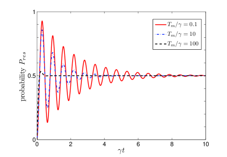
Figure 2: (Color online) The probability $P_{\textrm{res}}$ given in Eq. (2) is plotted vs the scaled time $\gamma t$ for different bath temperatures $T_{m}/\gamma=0.1$ (solid red line), $10$ (dash dotted blue line), and $100$ (dashed black line) in the resonant case $\Delta\omega/\gamma=0$. Other parameters are set as $\gamma=1$, $\xi/\gamma=5$, and $\Delta T/\gamma=0$.

The exponential rate $N(2\xi)\gamma/2$ is a function of the parameters $\xi$, $\gamma$, $T_{1}$, and $T_{2}$. Obviously, the parameter $N(2\xi)$ increases with the increase of the temperatures of the heat baths. In the low temperature limit, i.e., $T_{1}/(2\xi)\approx 0$ and $T_{2}/(2\xi)\approx 0$, we have $\bar{n}_{1}(2\xi)\approx 0$ and $\bar{n}_{2}(2\xi)\approx 0$, then $N(2\xi)\approx 1$. On the contrary, in the high temperature limit, i.e., $T_{1}/(2\xi)\gg 1$ and $T_{2}/(2\xi)\gg 1$, we have $\bar{n}_{1}(2\xi)\approx T_{1}/(2\xi)$ and $\bar{n}_{2}(2\xi)\approx T_{2}/(2\xi)$, then

$$N(2\xi)\approx\frac{T_{1}+T_{2}}{2\xi}+1\approx\frac{T_{m}}{\xi}.$$ (18)

The above equation means that in the high temperature limit, the rate $N(2\xi)$ is proportional to the mean temperature $T_{m}$ and does not depend on the temperature difference $\Delta T$. In Fig. 2, we plot the probability $P_{\textrm{res}}$ vs the scaled time $\gamma t$ for different bath temperatures $T_{m}$, here we assume that $T_{1}=T_{2}=T_{m}$. From Fig. 2, we can see that in the low temperature limit the probability increases with an initial oscillation. With the increase of the bath temperatures, the oscillation disappears gradually.

(2) The high temperature limit case, i.e., $T_{1},T_{2}\gg\varepsilon$. In this case, $\bar{n}_{1}(\varepsilon),\bar{n}_{2}(\varepsilon)\gg 1$, then we can make the approximations $\bar{n}_{1}(\varepsilon)\approx\bar{n}_{1}(\varepsilon)+1$ and $\bar{n}_{2}(\varepsilon)\approx\bar{n}_{2}(\varepsilon)+1$, which lead to $\Gamma_{23}\approx\Gamma_{32}$. Therefore from Eq. (15) we can obtain the time dependent probability

$$P_{\textrm{htl}}\left(t\right) \approx \frac{1}{2}-\frac{1}{2}\cos^{2}\theta e^{-\sin^{2}\theta N(\varepsilon)\gamma t}$$ (19)

$$-\frac{1}{2}\sin^{2}\theta\cos(\varepsilon t)e^{-\left(2\cos^{2}\theta\chi+\frac{1}{2}\sin^{2}\theta N(\varepsilon)\gamma\right)t},$$

where we introduce the parameter $N(\varepsilon)=\bar{n}_{1}(\varepsilon)+\bar{n}_{2}(\varepsilon)+1$ and the subscript “htl” stands for the high temperature limit. Obviously, the above probability $P_{\textrm{htl}}$ increases from an initial value $0$ to a steady-state value $1/2$. And the increase of $P_{\textrm{htl}}$ is not simply exponential. In Fig. 3, we plot the probability $P_{\textrm{htl}}$ vs the scaled time $\gamma t$ and the mixing angle $\theta$ in the high temperature limit. Since the probability (19) is a function of $\sin^{2}\theta$ and $\cos^{2}\theta$, therefore in Fig. 3 we only need to plot the probability in Eq. (19) for the negative detuning cases. Figure 3 shows that in the long time limit the probability reaches $1/2$ irrespective of the $\theta$. Note that here the mixing angle $0<\theta<\pi$. The cases of $0<\theta<\pi/2$ and $\pi/2<\theta<\pi$ mean the energy detuning $\Delta\omega>0$ and $\Delta\omega<0$, respectively. And the angle $\theta=\pi/2$ corresponds to the resonant case. Here we choose $0.1\pi<\theta<0.9\pi$, which corresponds to $6.2>\Delta\omega/\xi>-6.2$.

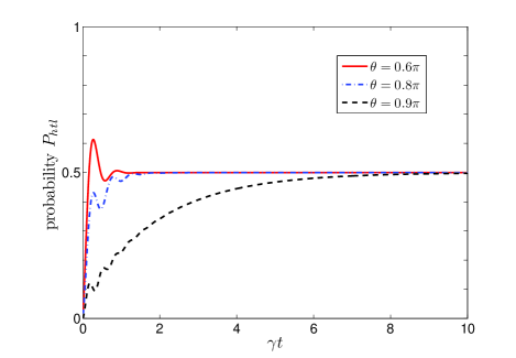
Figure 3: (Color online) The probability $P_{\textrm{htl}}$ given in Eq. (19) vs the scaled time $\gamma t$ for different mixing angle $\theta=0.6\pi$ (solid red line), $0.8\pi$ (dash dotted blue line), and $0.9\pi$ (dashed black line) at the high temperature limit $T_{m}/\gamma=100$. Other parameters are set as $\gamma=1$, $\xi/\gamma=5$, $\chi_{1}/\gamma=\chi_{2}/\gamma=0.01T_{m}$, and $\Delta T/\gamma=0$.

(3) The low temperature limit case, i.e., $T_{1},T_{2}\approx 0$. Now we can make the approximations $\bar{n}_{1}(\varepsilon)\approx 0$ and $\bar{n}_{2}(\varepsilon)\approx 0$, which lead to $\Gamma_{32}\approx 0$ and $\Gamma_{23}\approx\sin^{2}\theta~{}\gamma/2$. Then we obtain the probability

$$P_{\textrm{ltl}}(t) \approx \cos^{2}(\theta/2)\left(1-\cos\theta e^{-\sin^{2}\theta\gamma t}\right)$$ (20)

$$-\frac{1}{2}\sin^{2}\theta\cos(\varepsilon t)e^{-\frac{1}{2}\sin^{2}\theta\gamma t},$$

where the subscript “ltl” means the low temperature limit. In this case, the probability increases for an initial value $0$ to a steady-state value $\cos^{2}(\theta/2)$. In Fig. 4, we plot the probability $P_{\textrm{ltl}}$ vs the time $t$ for different mixing angles $\theta$ in the low temperature limit. Figure 4 shows that the probability $P_{\textrm{ltl}}$ increases from $0$ to a steady state value with the increase of the time $t$. In the short time, the probability experiences small oscillation. The steady state value decreases with the increase of the $\theta$. Actually, the obtained results are very reasonable from the viewpoint of energy conservation. For the case of $\theta<\pi/2$, the energy detuning $\Delta\omega>0$, we have $\omega_{1}>\omega_{2}$, then the energy emitted by TLS$1$ can excite more than one TLS$2$ into their excited state; For the case of $\theta>\pi/2$, we have $\Delta\omega<0$, we have $\omega_{1}<\omega_{2}$, then the energy emitted by TLS$1$ can only excite less than one TLS$2$ into the excited state. Therefore, it is understandable that the steady-state value of probability in low temperature increases as the parameter $\theta$ decreases.

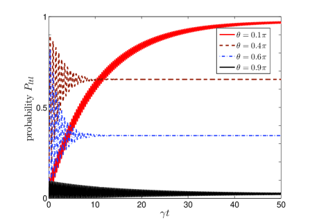
Figure 4: (Color online) The probability $P_{\textrm{ltl}}(t)$ given in Eq. (20) vs the scaled time $\gamma t$ for different mixing angle $\theta=0.1\pi$ (solid red line), $0.4\pi$ (dashed brown line), $0.6\pi$ (dash dotted blue line), and $0.9\pi$ (solid black line) at the low temperature limit $T_{m}/\gamma=1$. Other parameters are set as $\gamma=1$, $\xi/\gamma=5$, and $\Delta T/\gamma=0$.

IV.2 Steady state case

At steady state, the probability (15) becomes

$$P_{ss}=\frac{1}{2}\left(1+\frac{\cos\theta}{N(\varepsilon)}\right),$$ (21)

where the subscript “ss” stands for steady state and $N(\varepsilon)=\bar{n}_{1}(\varepsilon)+\bar{n}_{2}(\varepsilon)+1$. This steady-state probability is a very interesting result since it depends on the mixing angle $\theta$ and the bath temperatures $T_{1}$ and $T_{2}$ independently. It depends on the mixing angle $\theta$ and the bath temperatures $T_{1}$ and $T_{2}$ by $\cos\theta$ and $1/N(\varepsilon)$, respectively.

We first consider several special cases at steady state: (1) The resonant case, i.e., $\Delta\omega=0$. In this case, $\cos\theta=0$, then $P_{ss}=1/2$. In the resonant case, the steady-state probability $P_{ss}$ for single-excitation energy transfer is independence of the temperatures of the two heat baths. This result can also be understood from the following viewpoints: When $\sin(\theta/2)=\cos(\theta/2)=1/\sqrt{2}$, the eigenstates $|\lambda_{2}\rangle$ and $|\lambda_{3}\rangle$ become $|\lambda_{2}\rangle=(|eg\rangle+|ge\rangle)/\sqrt{2}$ and $|\lambda_{3}\rangle=(-|eg\rangle+|ge\rangle)/\sqrt{2}$. Therefore for any statistical mixture $\rho_{ss}=p_{2}\sigma_{22}+p_{3}\sigma_{33}$ of the two eigenstates $|\lambda_{2}\rangle$ and $|\lambda_{3}\rangle$, the probability for finding the two TLSs in state $|ge\rangle$ is $1/2$, where $p_{2}+p_{3}=1$ is the normalization condition. (2) The high temperature limit, i.e., $T_{1},T_{2}\gg\varepsilon$. In this case, $\bar{n}_{1}(\varepsilon)\gg 1$ and $\bar{n}_{2}(\varepsilon)\gg 1$, therefore $N(\varepsilon)\gg 1$, which leads to $P_{ss}\approx 1/2$. In fact, in the high temperature limit, the steady state of the TLSs should be $\rho_{s}\approx(\sigma_{22}+\sigma_{33})/2$, therefore according to Eq. (3) we know that the probability for finding the two TLSs in state $|ge\rangle$ is $1/2$. (3) The low temperature limit, i.e., $T_{1},T_{2}\ll\varepsilon$. In this case, $\bar{n}_{1}(\varepsilon)\approx 0$ and $\bar{n}_{2}(\varepsilon)\approx 0$, then $N(\varepsilon)\approx 1$, which means $P_{ss}=\cos^{2}(\theta/2)$. In Fig. 5, we plot the steady-state probability $P_{ss}$ in Eq. (21) vs the bath temperatures $T_{m}$.

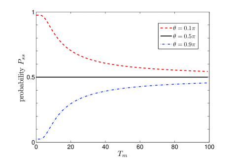
Figure 5: (Color online) The steady state probability $P_{ss}$ vs the bath temperature $T_{m}$ for different mixing angle $\theta=0.1\pi$ (dashed red line), $0.5$ (solid black line), and $0.9\pi$ (dash dotted blue line). Other parameters are set as $\gamma=1$, $\xi/\gamma=5$, and $\Delta T/\gamma=0$.

Figure 5 shows that, for the positive detuning case, i.e., $0<\theta<\pi/2$, the steady state probability $P_{ss}$ decreases from $1$ to $1/2$, but for the negative detuning case, i.e., $\pi/2<\theta<\pi$, the $P_{ss}$ increases from $0$ to $1/2$. For the resonant case, the $P_{ss}$ is $1/2$ irrespectively of the bath temperature $T_{1}=T_{2}=T_{m}$. In Fig. 6, we plot the steady-state probability $P_{ss}$ in Eq. (21) vs the mixing angle $\theta$.

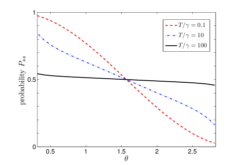
Figure 6: (Color online) The steady state probability $P_{ss}$ vs the mixing angle $\theta$ for different bath temperature $T_{m}/\gamma=0.1$ (dashed red line), $10$ (dash dotted blue line), and $100$ (solid black line). Other parameters are set as $\gamma=1$, $\xi/\gamma=5$, and $\Delta T/\gamma=0$.

Figure 6 shows that, in the high temperature case, the $P_{ss}$ becomes approximately a fixed value $1/2$ irrespective of the $\theta$. But in the low temperature case, the steady state probability $P_{ss}$ decreases with the increase of $\theta$. These results are consistent with the above analysis. Therefore, in the low temperature limit, we can improve the steady-state probability $P_{ss}$ via increasing the $\Delta\omega$.

In the above discussions of the steady-state probability, we have assumed the bath temperature difference $\Delta T$ is zero. Actually, we also study the dependence of the steady-state probability on the bath temperature difference $\Delta T$ in both the low and the high temperature limits. We found that the dependence of the probability on $\Delta T$ is negligibly small with the current parameters. This result is well understood from the following viewpoint: in the low temperature limit, we have $T_{1},T_{2}\ll\varepsilon$, therefore $\bar{n}_{1}(\varepsilon)\approx 0$ and $\bar{n}_{2}(\varepsilon)\approx 0$, $N(\varepsilon)\approx 1$, then $P_{ss}=\cos^{2}(\theta/2)$, which does not depends on the bath temperature difference $\Delta T$; On the other hand, in the high temperature limit, $T_{1},T_{2}\gg\varepsilon$, therefore $\bar{n}_{1}(\varepsilon)\gg 1$ and $\bar{n}_{2}(\varepsilon)\gg 1$, then

$$P_{ss}\approx\frac{1}{2}\left(1+\frac{\varepsilon\cos\theta}{2T_{m}}\right),$$ (22)

which is independent of the bath temperature difference $\Delta T$.

V Quantum entanglement between the donor and acceptor

In this section, we study the quantum entanglement between the donor and the acceptor with concurrence, which will be defined below. For a $2\times 2$ quantum system (two TLSs) with density matrix $\rho$ expressed in the bare state representation, its concurrence is defined as Wootters1998

$$C(\rho)=\max\{0,\sqrt{s_{1}}-\sqrt{s_{2}}-\sqrt{s_{3}}-\sqrt{s_{4}}\},$$ (23)

where $s_{i}$ ($i=1,2,3,4$) are the eigenvalues ($s_{1}$ being the largest one) of the matrix $\rho\tilde{\rho}$, where the operator $\tilde{\rho}$ is define as

$$\tilde{\rho}=(\sigma^{y}_{1}\otimes\sigma^{y}_{2})\rho^{\ast}(\sigma^{y}_{1}\otimes\sigma^{y}_{2})$$ (24)

with $\rho^{\ast}$ being the complex conjugate of $\rho$. Note that here $\sigma^{y}_{i}$ is the usual Pauli matrix pointing the $y$ axis. For the $2\times 2$ quantum system, the concurrences $C=0$ and $C=1$ mean the density matrix $\rho$ is an unentangled and maximally entangled states, respectively. Specially, for the “X”-class state with the density matrix

$$\rho=\left(\begin{array}[]{cccc}\rho_{11}&0&0&\rho_{14}\\ 0&\rho_{22}&\rho_{23}&0\\ 0&\rho_{32}&\rho_{33}&0\\ \rho_{41}&0&0&\rho_{44}\\ \end{array}\right)$$ (29)

expressed in the bare state representation, the concurrence is Zubairy1998

$$C(\rho)=\max\{0,2(|\rho_{23}|-\sqrt{\rho_{11}\rho_{44}}),2(|\rho_{14}|-\sqrt{\rho_{22}\rho_{33}})\}.$$ (30)

Now, for the present system, its density matrix $\rho$ can be expressed as the following form in the bare state representation,

$$\rho=\left(\begin{array}[]{cccc}\langle\tau_{11}\rangle&\langle\tau_{21}\rangle&\langle\tau_{31}\rangle&\langle\tau_{41}\rangle\\ \langle\tau_{12}\rangle&\langle\tau_{22}\rangle&\langle\tau_{32}\rangle&\langle\tau_{42}\rangle\\ \langle\tau_{13}\rangle&\langle\tau_{23}\rangle&\langle\tau_{33}\rangle&\langle\tau_{43}\rangle\\ \langle\tau_{14}\rangle&\langle\tau_{24}\rangle&\langle\tau_{34}\rangle&\langle\tau_{44}\rangle\\ \end{array}\right),$$ (35)

where the density matrix elements are defined as $\langle\tau_{ij}\rangle=\textrm{Tr}[\tau_{ij}\rho]=\textrm{Tr}[|\eta_{i}\rangle\langle\eta_{j}|\rho]=\langle\eta_{j}|\rho|\eta_{i}\rangle$ with the transition operator $\tau_{ij}=|\eta_{i}\rangle\langle\eta_{j}|$. Since the concurrence is defined in the bare state representation and the evolution of the system is expressed in the eigenstate representation. Therefore we need to obtain the transformation between the two representations. The density matrix elements in the eigenstate and bare state representations are expressed by $\langle\sigma_{ij}(t)\rangle$ and $\langle\tau_{ij}(t)\rangle$, respectively. Making using of Eq. (3), we can obtain the relations for diagonal density matrix elements

$$\left\langle\sigma_{11}(t)\right\rangle = \left\langle\tau_{11}(t)\right\rangle,\hskip 14.22636pt\left\langle\sigma_{44}(t)\right\rangle=\left\langle\tau_{44}(t)\right\rangle,$$

$$\left\langle\sigma_{22}(t)\right\rangle = \cos^{2}\left(\theta/2\right)\left\langle\tau_{22}(t)\right\rangle+\sin^{2}\left(\theta/2\right)\left\langle\tau_{33}(t)\right\rangle$$

$$+\frac{1}{2}\sin\theta\left(\left\langle\tau_{23}(t)\right\rangle+\left\langle\tau_{32}(t)\right\rangle\right),$$

$$\left\langle\sigma_{33}(t)\right\rangle = \sin^{2}\left(\theta/2\right)\left\langle\tau_{22}(t)\right\rangle+\cos^{2}\left(\theta/2\right)\left\langle\tau_{33}(t)\right\rangle$$ (36)

$$-\frac{1}{2}\sin\theta\left(\left\langle\tau_{23}(t)\right\rangle+\left\langle\tau_{32}(t)\right\rangle\right),$$

and the following off-diagonal element which will be useful below,

$$\left\langle\sigma_{23}(t)\right\rangle = \frac{1}{2}\sin\theta(\left\langle\tau_{33}(t)\right\rangle-\left\langle\tau_{22}(t)\right\rangle)$$ (37)

$$+\cos^{2}\left(\theta/2\right)\left\langle\tau_{23}(t)\right\rangle-\sin^{2}\left(\theta/2\right)\left\langle\tau_{32}(t)\right\rangle.$$

Correspondingly, we can obtain the inverse transform

$$\left\langle\tau_{22}(t)\right\rangle = \cos^{2}\left(\theta/2\right)\left\langle\sigma_{22}(t)\right\rangle+\sin^{2}\left(\theta/2\right)\left\langle\sigma_{33}(t)\right\rangle$$

$$-\frac{1}{2}\sin\theta\left(\left\langle\sigma_{23}(t)\right\rangle+\left\langle\sigma_{32}(t)\right\rangle\right),$$

$$\left\langle\tau_{33}(t)\right\rangle = \sin^{2}\left(\theta/2\right)\left\langle\sigma_{22}(t)\right\rangle+\cos^{2}\left(\theta/2\right)\left\langle\sigma_{33}(t)\right\rangle$$

$$+\frac{1}{2}\sin\theta\left(\left\langle\sigma_{23}(t)\right\rangle+\left\langle\sigma_{32}(t)\right\rangle\right),$$

$$\left\langle\tau_{23}(t)\right\rangle = -\sin^{2}\left(\theta/2\right)\left\langle\sigma_{32}(t)\right\rangle+\cos^{2}\left(\theta/2\right)\left\langle\sigma_{23}(t)\right\rangle$$ (38)

$$+\frac{1}{2}\sin\theta\left(\left\langle\sigma_{22}(t)\right\rangle-\left\langle\sigma_{33}(t)\right\rangle\right).$$

Also here we only express explicitly the elements which will be used below.

In order to calculate the concurrence of the system, we need to know its density matrix in the bare representation for a given initial state. Fortunately, the evolution relation from $\langle\tau_{ij}(0)\rangle$ to $\langle\tau_{ij}(t)\rangle$ can be obtained through the following process

$$\langle\tau_{ij}(0)\rangle\rightarrow\langle\sigma_{ij}(0)\rangle\rightarrow\langle\sigma_{ij}(t)\rangle\rightarrow\langle\tau_{ij}(t)\rangle.$$ (39)

Concretely, the transformation relations $\langle\tau_{ij}(0)\rangle\rightarrow\langle\sigma_{ij}(0)\rangle$ and $\langle\sigma_{ij}(t)\rangle\rightarrow\langle\tau_{ij}(t)\rangle$ are determined by Eqs. (36), (37) and (38), and the evolution relation $\langle\sigma_{ij}(0)\rangle\rightarrow\langle\sigma_{ij}(t)\rangle$ is determined by Eq. (III). In terms of Eqs. (III), (36), (37),  (38), and (39), we can obtain the following relation

$$\left\langle\tau_{23}\left(t\right)\right\rangle = \left[\frac{1}{2}\sin\theta\frac{\Gamma_{32}-\Gamma_{23}}{\Gamma_{23}+\Gamma_{32}}+\sin\theta\frac{(\cos^{2}\left(\theta/2\right)\Gamma_{23}-\sin^{2}\left(\theta/2\right)\Gamma_{32})}{\Gamma_{23}+\Gamma_{32}}e^{-2\left(\Gamma_{23}+\Gamma_{32}\right)t}\right.$$ (40)

$$\left.-\frac{1}{2}\sin\theta e^{-\left(\cos^{2}\theta\Pi_{1}+\Gamma_{23}+\Gamma_{32}\right)t}\left(e^{i\varepsilon t}\cos^{2}\left(\theta/2\right)-e^{-i\varepsilon t}\sin^{2}\left(\theta/2\right)\right)\right]\left\langle\tau_{22}\left(0\right)\right\rangle$$

$$+\left[\frac{1}{2}\sin\theta\frac{\Gamma_{32}-\Gamma_{23}}{\Gamma_{23}+\Gamma_{32}}+\sin\theta\frac{\sin^{2}\left(\theta/2\right)\Gamma_{23}-\cos^{2}\left(\theta/2\right)\Gamma_{32})}{\Gamma_{23}+\Gamma_{32}}e^{-2\left(\Gamma_{23}+\Gamma_{32}\right)t}\right.$$

$$\left.+\frac{1}{2}\sin(\theta)e^{-\left(\cos^{2}\theta\Pi_{1}+\Gamma_{23}+\Gamma_{32}\right)t}\left(e^{i\varepsilon t}\cos^{2}\left(\theta/2\right)-e^{-i\varepsilon t}\sin^{2}\left(\theta/2\right)\right)\right]\left\langle\tau_{33}\left(0\right)\right\rangle$$

$$+\left[(\sin^{4}\left(\theta/2\right)e^{-i\varepsilon t}+\cos^{4}\left(\theta/2\right)e^{i\varepsilon t})e^{-\left(\cos^{2}\theta\Pi_{1}+\Gamma_{23}+\Gamma_{32}\right)t}+\frac{1}{2}\sin^{2}\theta e^{-2\left(\Gamma_{23}+\Gamma_{32}\right)t}\right]\left\langle\tau_{23}\left(0\right)\right\rangle$$

$$+\frac{1}{2}\sin^{2}\theta\left(e^{-2\left(\Gamma_{23}+\Gamma_{32}\right)t}-e^{-\left(\cos^{2}\theta\Pi_{1}+\Gamma_{23}+\Gamma_{32}\right)t}\cos(\varepsilon t)\right)\left\langle\tau_{32}\left(0\right)\right\rangle.$$

Now, we obtain the evolution relation of the density matrix elements in the bare state representation. Since the expressions are very complex, here we only show the matrix elements which will be used in the following. Based on these evolutionary matrix elements, we can write out the density matrix of the system in bare state representation at time $t$ once the initial state is given, and then we can obtain the concurrence of the density matrix. In what follows, we will discuss the entanglement dynamics and steady-state entanglement.

V.1 Entanglement dynamics

In the process of single-excitation energy transfer from the donor to the acceptor, the single excitation energy is initially possessed by the donor and the acceptor is in its ground state. Therefore the initial state of the system is

$$|\psi(0)\rangle=|eg\rangle=|\eta_{2}\rangle,$$ (41)

which means the initial conditions are that all matrix elements are zero except $\langle\tau_{22}(0)\rangle=1$. According to Eq. (40), we know that the density matrix $\rho(t)$ of the system belongs to the so-called $X$-class state. Then the concurrence can be obtained with Eq. (30)

$$C(t) = 2\left|\left[\frac{1}{2}\sin\theta\frac{\Gamma_{32}-\Gamma_{23}}{\Gamma_{23}+\Gamma_{32}}\right.\right.$$ (42)

$$\left.\left.+\sin\theta\frac{(\cos^{2}\left(\theta/2\right)\Gamma_{23}-\sin^{2}\left(\theta/2\right)\Gamma_{32})}{\Gamma_{23}+\Gamma_{32}}e^{-2\left(\Gamma_{23}+\Gamma_{32}\right)t}\right.\right.$$

$$\left.\left.-\frac{1}{2}\sin\theta e^{-\left(\cos^{2}\theta\Pi_{1}+\Gamma_{23}+\Gamma_{32}\right)t}\right.\right.$$

$$\left.\left.\times\left(e^{i\varepsilon t}\cos^{2}\left(\theta/2\right)-e^{-i\varepsilon t}\sin^{2}\left(\theta/2\right)\right)\right]\right|.$$

In what follows, we consider three special cases of interest: (1) The resonant case, i.e., $\omega_{1}=\omega_{2}=\omega_{m}$, that is $\Delta\omega=0$. Then the mixing angle $\theta=\pi/2$ and the energy separation $\varepsilon=2\xi$, thus we obtain

$$C_{\textrm{res}}(t) \approx \left|\frac{1}{N(2\xi)}\left(1-e^{-N(2\xi)\gamma t}\right)+i\sin(\varepsilon t)e^{-\frac{1}{2}N(2\xi)\gamma t}\right|,$$ (43)

where $N(2\xi)=\bar{n}_{1}(2\xi)+\bar{n}_{2}(2\xi)+1$. From Eq. (43), we find that the concurrence $C_{\textrm{res}}(t)$ increases from zero to a steady state value $1/N(2\xi)$ with the increase of the time $t$. Clearly, the steady state concurrence $1/N(2\xi)$ decreases from one to zero as the temperature $T_{m}$ increases from zero to infinite.

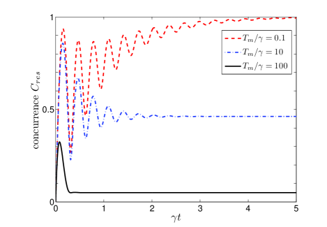
Figure 7: (Color online) The concurrence $C_{\textrm{res}}$ in Eq. (43) vs the scaled time $\gamma t$ for different bath temperature $T_{m}/\gamma=0.1$ (dashed red line), $10$ (dash dotted blue line), and $100$ (solid black line) in the resonant case $\Delta\omega/\gamma=0$. Other parameters are set as $\gamma=1$, $\xi/\gamma=5$, and $\Delta T/\gamma=0$.

In Fig. 7, we plot the concurrence (43) in the resonant case vs the scaled time $\gamma t$ and for different heat bath average temperatures $T_{m}$. Figure 7 shows the results as we analyze above.

(2) The high temperature limit, i.e., $T_{1},T_{2}\gg\varepsilon$. In this case, $\bar{n}_{1}(\varepsilon),\bar{n}_{2}(\varepsilon)\gg 1$, then we can have the approximate relations $\bar{n}_{1}(\varepsilon)\approx\bar{n}_{1}(\varepsilon)+1$ and $\bar{n}_{2}(\varepsilon)\approx\bar{n}_{2}(\varepsilon)+1$, which lead to $\Gamma_{23}\approx\Gamma_{32}$. Then the concurrence (42) becomes

$$C_{\textrm{htl}}(t) \approx \left|\frac{\sin(2\theta)}{2}e^{-\sin^{2}\theta N(\varepsilon)\gamma t}-\sin\theta e^{-\left(2\cos^{2}\theta\chi+\frac{1}{2}\sin^{2}\theta N(\varepsilon)\gamma\right)t}\right.$$ (44)

$$\left.\times\left(e^{i\varepsilon t}\cos^{2}\left(\theta/2\right)-e^{-i\varepsilon t}\sin^{2}\left(\theta/2\right)\right)\right|.$$

The expression of the concurrence (44) in the high temperature limit is not simple as that of the resonant case, but we can still observe the two points: The first is that the dependence of the concurrence on the angle $\theta$ is approximately $\sin\theta$; and the second is that the steady-state concurrence is zero, which means there is no quantum entanglement between the donor and the acceptor. This result can also be seen from the density operator of the steady state for the donor and the acceptor. In the high temperature limit, the steady state density matrix of the donor and the acceptor is $\rho\approx(|eg\rangle\langle eg|+|ge\rangle\langle ge|)/2$, which is an unentangled state. Physically, this result is direct since the quantum systems will transit to classical systems in the high temperature limit. In Fig. 8, we plot the concurrence given by Eq. (44) vs the evolution time $t$ for different mixing angles $\theta$. Figure 8 shows that the concurrence experiences an increase from zero to a maximal value and then decreases to a steady state value with the scaled time $\gamma t$.

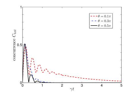
Figure 8: (Color online) The concurrence $C_{\textrm{htl}}$ in Eq. (44) vs the scaled evolution time $\gamma t$ for different mixing angle $\theta=0.1\pi$ (dashed red line), $0.3\pi$ (dashed blue line), and $0.5\pi$ (solid black line) in the high temperature limit $T_{m}/\gamma=100$. Other parameters are set as $\gamma=1$, $\xi/\gamma=5$, $\chi_{1}/\gamma=\chi_{2}/\gamma=0.01T_{m}$, and $\Delta T/\gamma=0$.

(3) The low temperature limit, i.e., $T\approx 0$. Now we can approximately have $\bar{n}(\varepsilon)\approx 0$, which lead to $\Gamma_{32}\approx 0$ and $\Gamma_{23}\approx\sin^{2}\theta\gamma/2$. Then the concurrence (42) becomes

$$C_{\textrm{ltl}}(t) \approx \sin\theta\left|1-2\cos^{2}(\theta/2)e^{-\sin^{2}\theta\gamma t}+e^{-\frac{1}{2}\sin^{2}\theta\gamma t}\right.$$ (45)

$$\left.\times\left(e^{i\varepsilon t}\cos^{2}\left(\theta/2\right)-e^{-i\varepsilon t}\sin^{2}\left(\theta/2\right)\right)\right|,$$

where the subscript “ltl” stands for low temperature limit. Similar to the high temperature limit, the increase of the concurrence is also not simply exponential. The concurrence increases from zero to a steady state value $\sin\theta$ with the increase of the scaled time $t$, which means the concurrence at long time limit is irrespective of the sign of the detuning. This long lived entanglement is much larger than that of the high temperature limit. We can also see the steady state concurrence from the viewpoint of quantum noise. When $T\approx 0$, the steady state of the donor and the acceptor is $\rho\approx|\lambda_{3}\rangle\langle\lambda_{3}|$ with concurrence $\sin\theta$. In Fig. 9, we plot the concurrence given by Eq. (45) vs the evolution time $t$ and the mixing angle $\theta$. Figure 9 shows that the concurrence increases from zero to a steady state value with the scaled time $t$.

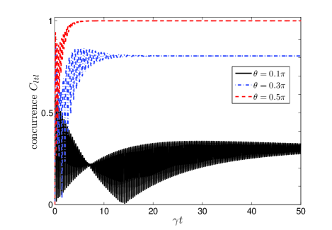
Figure 9: (Color online) The concurrence $C_{\textrm{ltl}}$ in Eq. (45) vs the scaled evolution time $\gamma t$ for different mixing angle $\theta=0.1\pi$ (solid black line), $0.3\pi$ (dash dotted blue line), and $0.5\pi$ (dashed red line) is plotted in the low temperature limit $T_{m}/\gamma=0.01$. Other parameters are set as $\gamma=1$, $\xi/\gamma=5$, $\chi_{1}/\gamma=\chi_{2}/\gamma=0.01T_{m}$, and $\Delta T/\gamma=0$.

V.2 Steady state entanglement

From Eq. (42), it is straightforward to obtain the steady state concurrence between the donor and the acceptor,

$$C_{ss} = \frac{\sin\theta}{N(\varepsilon)}.$$ (46)

In the high temperature limit, we have $C_{\textrm{htl}}(\infty)\approx 0$, and in the low temperature limit, we have $C_{\textrm{ltl}}(\infty)\approx\sin\theta$. For a general state, it is interesting to point out that the steady state concurrence $C_{ss}$ depends on the temperature $T_{m}$ and the angle $\theta$ independently. For a given $\theta$, the dependence on $T_{m}$ is inverse proportional to $N(\varepsilon)$, and for a given $T_{m}$, the dependence on $\theta$ is $\sin\theta$. In Fig. 10, we plot the concurrence given by Eq. (46) vs the temperature $T_{m}$ for different mixing angles $\theta$.

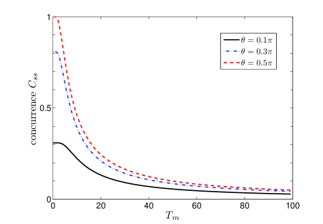
Figure 10: (Color online) The steady state concurrence $C_{ss}$ vs the bath temperature $T_{m}$ for different mixing angle $\theta=0.1\pi$ (solid black line), $0.3$ (dash dotted blue line), and $0.5\pi$ (dashed red line). Other parameters are set as $\gamma=1$, $\xi/\gamma=5$, and $\Delta T/\gamma=0$.

Figure 10 shows that the steady state concurrence decreases with the increase of the temperature $T_{m}$. In Fig. 11, we plot the concurrence given by Eq. (46) vs the mixing angle $\theta$ for different average bath temperature $T_{m}$. Figure 11 shows that the dependence of the concurrence on the mixing angle $\theta$ decreases with the increase of the average bath temperature $T_{m}$. Moreover, from Eq. (46), we can also see that the steady-state concurrence is independent of $\Delta T$ at the high temperature limit.

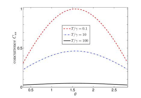
Figure 11: (Color online) The steady state concurrence $C_{ss}$ vs the mixing angle $\theta$ for different bath temperature $T_{m}/\gamma=0.1$ (dashed red line), $10$ (dash dotted blue line), and $100$ (solid black line). Other parameters are set as $\gamma=1$, $\xi/\gamma=5$, and $\Delta T/\gamma=0$.

VI concluding with remarks

In conclusion, we have studied analytically coherent single-excitation energy transfer in a dimer consisting of a donor and an acceptor modeled by two TLSs, which are immersed in two independent heat baths. Special attention is paid to the effect on the single-excitation energy transfer probability of the energy detuning and the heat bath temperatures of the two TLSs. It has been found that, the probability for single-excitation energy transfer largely depends on the energy detuning in the low temperature limit. Concretely, the positive and negative energy detunings can increase and decrease the probability, respectively. In the high temperature limit, however, the effect of the energy detuning on the probability is negligibly small. We have also found that the probability is negligibly dependence on the bath temperature difference in the low and high temperature limits. We have also studied analytically quantum entanglement in the dimer system through calculating quantum concurrence. It was found that quantum entanglement can be created during the process of excitation energy transfer. The steady state entanglement between the donor and the acceptor decreases with the increasing of the bath temperature. And the dependence of the steady state concurrence on the energy detuning is proportional to the sine function of the mixing angle and irrespective of the bath temperatures. Moreover, we have found that the dependence of the steady state concurrence on the bath temperature difference is negligibly small with the current parameters.

Finally, we give two remarks on the above obtained results: First, we should distinguish the present work from dynamic disentanglement suddenly or asymptotically (e.g., Refs. YuTing ; Almeida ; Ficek ; FQWang ; Dubi ; BAn ; Ann ; ZheSun ; HZheng ; James ; Bellomo ; Davidovich ; Ban ). Mainly, there are three points of difference between the two cases: the initial state, the coupling between the two TLSs, and the coupling form between the TLSs and their heat baths. In dynamic disentanglement, the two TLSs is initially prepared in an entanglement state, there is no coupling between the two TLSs, and the coupling form of the TLSs with their heat baths is off-diagonal. But in the present work, initially the two TLSs are unentangled, there is a dipole-dipole interaction between the two TLSs, and the coupling form of the TLSs with their heat baths is diagonal. Certainly, the results also differ. In entanglement sudden death, the two TLSs disentangle to zero suddenly. But in this work, steady state entanglement is created.

Second, in this work, we only address the problem about how is the dynamics of the created quantum entanglement in the process of excitation energy transfer Scholak . But we do not address the question about the relation between initially prepared quantum entanglement among the pigments and the efficiency for single-excitation energy transfer. Just as in quantum information science, quantum entanglement is considered an important resource since it can be used to enhance the efficiency of quantum information protocols. Therefore it remains a question whether initially prepared quantum entanglement can enhance the efficiency of excitation energy transfer.

Appendix A Derivation of quantum master equation (7)

In this appendix, we present a detailed derivation of quantum master equation (7). Let us start from the Hamiltonian (1) of the total system. In the interaction picture with respect to the Hamiltonian

$$H_{0}=H_{\textrm{TLSs}}+H_{B},$$ (47)

the interaction Hamiltonian (6) becomes

$$H_{I}(t) = \sigma_{11}B_{11}(t)+\sigma_{22}B_{22}(t)+\sigma_{33}B_{33}(t)$$ (48)

$$+\sigma_{23}e^{i\varepsilon t}B_{23}(t)+\sigma_{32}e^{-i\varepsilon t}B^{{\dagger}}_{23}(t),$$

through introducing the following noise operators:

$$B_{11}(t) = A(t)+B(t),$$

$$B_{22}(t) = \cos^{2}(\theta/2)A(t)+\sin^{2}(\theta/2)B(t),$$

$$B_{33}(t) = \sin^{2}(\theta/2)A(t)+\cos^{2}(\theta/2)B(t),$$

$$B_{23}(t) = \frac{\sin\theta}{2}\left(\sum_{k}g_{2k}b_{k}e^{-i\omega_{bk}t}-\sum_{j}g_{1j}a_{j}e^{-i\omega_{aj}t}\right),$$ (49)

with

$$A(t) \equiv e^{iH^{(a)}_{B}t}A(0)e^{-iH^{(a)}_{B}t}$$

$$= \sum_{j}g_{1j}(a_{j}^{\dagger}e^{i\omega_{aj}t}+a_{j}e^{-i\omega_{aj}t}),$$

$$B(t) \equiv e^{iH^{(b)}_{B}t}B(0)e^{-iH^{(b)}_{B}t}$$ (50)

$$= \sum_{k}g_{2k}(b_{k}^{\dagger}e^{i\omega_{bk}t}+b_{k}e^{-i\omega_{bk}t}).$$

Obviously, $A(t)$ and $B(t)$ are Hermitian operators. Note that in Eq. (48) we have made rotating wave approximation.

Under the Born-Markov approximation, the master equation reads Breuer

$$\dot{\rho}_{S}=-\int_{0}^{\infty}d\tau\textrm{Tr}_{B}[H_{I}(t),[H_{I}(t-\tau),\rho_{S}\otimes\rho_{B}]],$$ (51)

where $\textrm{Tr}_{B}$ stands for tracing over the degrees of freedom of the heat baths. The density matrix $\rho_{B}\equiv\rho^{(a)}_{th}\otimes\rho^{(b)}_{th}$ of the heat baths means the two independent heat baths being in thermal equilibrium,

$$\rho^{(a)}_{th} = Z^{-1}_{A}\exp(-\beta_{1}H^{(a)}_{B}),$$

$$\rho^{(b)}_{th} = Z^{-1}_{B}\exp(-\beta_{2}H^{(b)}_{B}),$$ (52)

where we denote the partition functions $Z_{A}=\textrm{Tr}_{B_{a}}[\exp(-\beta_{1}H^{(a)}_{B})]$ and $Z_{B}=\textrm{Tr}_{B_{b}}[\exp(-\beta_{2}H^{(b)}_{B})]$ with $\beta_{1}=1/T_{1}$ and $\beta_{2}=1/T_{2}$ being respectively the inverse temperatures of the heat baths of the TLS$1$ and TLS$2$.

By using Eqs. (48) and (51) and making rotating wave approximation, we can obtain the following quantum master equation

$$\dot{\rho}_{S} = \sigma_{32}\rho_{S}\sigma_{23}\int_{0}^{\infty}e^{-i\varepsilon t}\langle B_{23}(-\tau)B^{{\dagger}}_{23}(0)\rangle d\tau$$ (53)

$$+\sigma_{23}\rho_{S}\sigma_{32}\int_{0}^{\infty}e^{i\varepsilon t}\langle B^{{\dagger}}_{23}(-\tau)B_{23}(0)\rangle d\tau$$

$$-\sigma_{22}\rho_{S}\int_{0}^{\infty}e^{i\varepsilon t}\langle B_{23}(0)B^{{\dagger}}_{23}(-\tau)\rangle d\tau$$

$$-\sigma_{33}\rho_{S}\int_{0}^{\infty}e^{-i\varepsilon t}\langle B^{{\dagger}}_{23}(0)B_{23}(-\tau)\rangle d\tau$$

$$+\sum_{m,n=1,2,3}\sigma_{mm}\rho_{S}\sigma_{nn}\int_{0}^{\infty}\langle B_{nn}(-\tau)B_{mm}(0)\rangle d\tau$$

$$-\sum_{n=1,2,3}\sigma_{nn}\rho_{S}\int_{0}^{\infty}\langle B_{nn}(0)B_{nn}(-\tau)\rangle d\tau$$

$$+h.c.,$$

where the correlation functions for the bath operators are defined as $\langle X(t)Y(t^{\prime})\rangle\equiv\textrm{Tr}_{B}[X(t)Y(t^{\prime})\rho_{B}]$. Notice that here we use the property $\langle X(t)Y(t^{\prime})\rangle=\langle X(t-t^{\prime})Y(0)\rangle=\langle X(0)Y(t^{\prime}-t)\rangle$ of the correlation functions for the bath operators. To derive the quantum master equation we need to calculate the Fourier transform of the correlation functions in Eq. (53). For simplicity, here we only keep the real parts of the Fourier transforms of the correlation functions and neglect their imaginary parts since the imaginary parts only contribute to the Lamb shifts, which are neglected in this work. According to Eqs. (A), (50), and (52), we can express the Fourier transforms for the correlation functions in Eq. (53) as follows:

$$\int_{0}^{\infty}d\tau\langle B_{11}(0)B_{11}(-\tau)\rangle = \int_{0}^{\infty}d\tau\langle B_{11}(-\tau)B_{11}(0)\rangle^{\ast}$$

$$= D_{A}+D_{B},$$

$$\int_{0}^{\infty}d\tau\langle B_{22}(0)B_{22}(-\tau)\rangle = \int_{0}^{\infty}d\tau\langle B_{22}(-\tau)B_{22}(0)\rangle^{\ast}$$

$$= \cos^{4}(\theta/2)D_{A}+\sin^{4}(\theta/2)D_{B},$$

$$\int_{0}^{\infty}d\tau\langle B_{33}(0)B_{33}(-\tau)\rangle = \int_{0}^{\infty}d\tau\langle B_{33}(-\tau)B_{33}(0)\rangle^{\ast}$$

$$= \sin^{4}(\theta/2)D_{A}+\cos^{4}(\theta/2)D_{B},$$

$$\int_{0}^{\infty}d\tau\langle B_{22}(-\tau)B_{11}(0)\rangle = \int_{0}^{\infty}d\tau\langle B_{11}(-\tau)B_{22}(0)\rangle$$

$$= \cos^{2}(\theta/2)D_{A}^{\ast}+\sin^{2}(\theta/2)D_{B}^{\ast},$$

$$\int_{0}^{\infty}d\tau\langle B_{33}(-\tau)B_{11}(0)\rangle = \int_{0}^{\infty}d\tau\langle B_{11}(-\tau)B_{33}(0)\rangle$$

$$= \sin^{2}(\theta/2)D_{A}^{\ast}+\cos^{2}(\theta/2)D_{B}^{\ast},$$

$$\int_{0}^{\infty}d\tau\langle B_{33}(-\tau)B_{22}(0)\rangle = \int_{0}^{\infty}d\tau\langle B_{22}(-\tau)B_{33}(0)\rangle$$ (54)

$$= \frac{1}{4}\sin^{2}(\theta/2)\left(D_{A}^{\ast}+D_{B}^{\ast}\right),$$

where the parameters are introduced as

$$D_{A} = \int_{0}^{\infty}d\tau\langle A(0)A(-\tau)\rangle,\hskip 5.69046ptD_{B}=\int_{0}^{\infty}d\tau\langle B(0)B(-\tau)\rangle,$$

$$D^{\ast}_{A} = \int_{0}^{\infty}d\tau\langle A(-\tau)A(0)\rangle,\hskip 5.69046ptD^{\ast}_{B}=\int_{0}^{\infty}d\tau\langle B(-\tau)B(0)\rangle.$$

Since the noise operators $B_{nn}$ $(n=1,2,3)$ are Hermitian operators, then we have the relations

$$\int_{0}^{\infty}d\tau\langle B_{nn}(-\tau)B_{mm}(0)\rangle=\int_{0}^{\infty}d\tau\langle B_{mm}(0)B_{nn}(-\tau)\rangle^{\ast}.$$

Therefore we can know all the diagonal correlation functions in Eq. (53) as long as we obtain the expression of $D_{A}$ and $D_{B}$. According to Eqs. (50) and  (52), we can calculate the expression of $D_{A}$ as follows,

$$D_{A} = \sum_{j}g_{1j}^{2}\langle a_{j}^{{\dagger}}a_{j}\rangle\int_{0}^{\infty}d\tau e^{i\omega_{aj}\tau}$$ (57)

$$+\sum_{j}g_{1j}^{2}\langle a_{j}a_{j}^{{\dagger}}\rangle\int_{0}^{\infty}d\tau e^{-i\omega_{aj}\tau}$$

$$= \sum_{j}g_{1j}^{2}\langle a_{j}^{{\dagger}}a_{j}\rangle\left[\pi\delta(\omega_{aj})+i\mathbf{P}\frac{1}{\omega_{aj}}\right]$$

$$+\sum_{j}g_{1j}^{2}\langle a_{j}a_{j}^{{\dagger}}\rangle\left[\pi\delta(\omega_{aj})-i\mathbf{P}\frac{1}{\omega_{aj}}\right]$$

$$= \textrm{Re}[D_{A}]+i\textrm{Im}[D_{A}],$$

where

$$\textrm{Re}[D_{A}] = \lim_{\omega\rightarrow 0^{+}}\pi\varrho_{1}\left(\omega\right)g_{1}^{2}\left(\omega\right)\left[2\bar{n}_{1}\left(\omega\right)+1\right].$$ (58)

Note that in the third line of Eq. (57) we have used the formula:

$$\int_{0}^{\infty}d\tau e^{\pm i\omega\tau}=\pi\delta\left(\omega\right)\pm i\mathbf{P}\frac{1}{\omega},$$ (59)

where the sign “$\mathbf{P}$” stands for the usual principal part integral. Similarly, we can obtain the expression of $\textrm{Re}[D_{B}]$,

$$\textrm{Re}[D_{B}] = \lim_{\omega\rightarrow 0^{+}}\pi\varrho_{2}\left(\omega\right)g_{2}^{2}\left(\omega\right)\left[2\bar{n}_{2}\left(\omega\right)+1\right].$$ (60)

Here $\varrho_{1}(\omega)$ and $\varrho_{2}(\omega)$ are the densities of state of the heat baths of the TLS$1$ and TLS$2$, respectively. And $\bar{n}_{1}(\omega)=1/[\exp(\beta_{1}\omega)-1]$ and $\bar{n}_{2}(\omega)=1/[\exp(\beta_{2}\omega)-1]$ are the average thermal excitation numbers. Using the same method we can obtain the following expressions:

$$\textrm{Re}\left[\int_{0}^{\infty}d\tau e^{i\varepsilon\tau}\langle B_{23}(0)B^{{\dagger}}_{23}(-\tau)\rangle\right]$$

$$= \textrm{Re}\left[\int_{0}^{\infty}d\tau e^{-i\varepsilon\tau}\langle B_{23}(-\tau)B^{{\dagger}}_{23}(0)\rangle\right]$$

$$= \frac{\pi}{4}\sin^{2}\theta[\varrho_{1}(\varepsilon)g_{1}^{2}(\varepsilon)(\bar{n}_{1}(\varepsilon)+1)+\varrho_{2}(\varepsilon)g_{2}^{2}(\varepsilon)(\bar{n}_{2}(\varepsilon)+1)]$$

and

$$\textrm{Re}\left[\int_{0}^{\infty}d\tau e^{-i\varepsilon\tau}\langle B^{{\dagger}}_{23}(0)B_{23}(-\tau)\rangle\right]$$ (62)

$$= \textrm{Re}\left[\int_{0}^{\infty}d\tau e^{i\varepsilon\tau}\langle B^{{\dagger}}_{23}(-\tau)B_{23}(0)\rangle\right]$$

$$= \frac{\pi}{4}\sin^{2}\theta[\varrho_{1}(\varepsilon)g_{1}^{2}(\varepsilon)\bar{n}_{1}(\varepsilon)+\varrho_{2}(\varepsilon)g_{2}^{2}(\varepsilon)\bar{n}_{2}(\varepsilon)].$$

By substituting these correlation functions into Eq. (53) and returning to the Schrödinger picture, we can obtain quantum master equation (7).

References

- (1) R. E. Blankenship, Molecular Mechanisms of Photosynthesis (Blackwell Science, Oxford, 2002).
- (2) V. May and O. Kühn, Charge and Energy Transfer Dynamics in Molecular Systems 2nd ed. (Wiley-VCH Verlag, Berlin, 2004).
- (3) G. R. Fleming and R. van Grondelle, Phys. Today 47, 48 (1994).
- (4) Y. C. Cheng and G. R. Fleming, Annu. Rev. Phys. Chem. 60, 241 (2009).
- (5) T. Renger, Photosynth Rev. 102, 471 (2009).
- (6) H. Lee, Y. C. Cheng, and G. R. Fleming, Science 316, 1462 (2007).
- (7) G. S. Engel, T. R. Calhoun, E. L. Read, T. K. Ahn, T. Mancal, Y. C. Cheng, R. E. Blankenship, and G, R. Fleming, Nature (London) 446, 782 (2007).
- (8) T. Förster, Ann. Phys. 2, 55 (1948).
- (9) A. Ishizaki and G. R. Fleming, J. Chem. Phys. 130, 234110 (2009); 130, 234111 (2009).
- (10) S. Jang, Y. C. Cheng, D. R. Reichman, and J. D. Eaves, J. Chem. Phys. 129, 101104 (2008).
- (11) B. Palmieri, D. Abramavicius, and S. Mukamel, J. Chem. Phys. 130, 204512 (2009).
- (12) M. Mohseni, P. Rebentrost, S. Lloyd, and A. Aspuru-Guzik, J. Chem. Phys. 129, 174106 (2008).
- (13) P. Rebentrost, M. Mohseni, I. Kassal, S. Lloyd, and A. Aspuru-Guzik, New J. Phys. 11, 033003 (2009).
- (14) P. Rebentrost, M. Mohseni, and A. Aspuru-Guzik, J. Phys. Chem. B 113, 9942 (2009).
- (15) P. Rebentrost, R. Chakraborty, and A. Aspuru-Guzik. J. Chem. Phys. 131, 184102 (2009).
- (16) M. B. Plenio and S. F. Huelga, New J. Phys. 10, 113019 (2008).
- (17) F. Caruso, A. W. Chin, A. Datta, S. F. Huelga, and M. B. Plenio, J. Chem. Phys. 131, 105106 (2009);
- (18) A. Olaya-Castro, C. F. Lee, F. F. Olsen, and N. F. Johnson, Phys. Rev. B 78, 085115 (2008).
- (19) F. Fassioli, A. Nazir, and A. Olaya-Castro, J. Phys. Chem. Lett. 1, 2139 (2010).
- (20) A. Nazir, Phys. Rev. Lett. 103, 146404 (2009).
- (21) A. Yu. Smirnov, L. G. Mourokh, and F. Nori, J. Chem. Phys. 130, 235105 (2009); P. K. Ghosh, A. Yu. Smirnov, and F. Nori, J. Chem. Phys. 131, 035102 (2009); A. Yu. Smirnov, S. Savel’ev, and F. Nori, Phys. Rev. E 80, 011916 (2009); A. Yu. Smirnov, L. G. Mourokh, P. K. Ghosh, and F. Nori, J. Phys. Chem. C. 113, 21218 (2009).
- (22) X. T. Liang, W. M. Zhang, and Y. Z. Zhuo, Phys. Rev. E 81, 011906 (2010).
- (23) S. Yang, D. Z. Xu, Z. Song, and C. P. Sun, J. Chem. Phys. 132, 234501 (2010).
- (24) S. J. Bell, Speakable and Unspeakable in Quantum Mechanics (Cambridge University Press, Cambridge, 1987).
- (25) A. Einstein, B. Podolsky, and N. Rosen, Phys. Rev. 41, 777 (1935).
- (26) M. A. Nielsen and I. L. Chuang, Quantum Computation and Quantum Information (Cambridge University Press, Cambridge, 2000).
- (27) X. F. Qian, Y. Li, Y. Li, Z. Song, and C. P. Sun, Phys. Rev. A 72, 062329 (2005).
- (28) H. J. Briegel and S. Popescu, arXiv:0806.4552.
- (29) J. Cai, G. G. Guerreschi, and H. J. Briegel, Phys. Rev. Lett. 104, 220502 (2010).
- (30) M. Thorwart, J. Eckel, J. H. Reina, P. Nalbach, and S. Weiss, Chem. Phys. Lett. 478, 234 (2009).
- (31) M. Sarovar, A. Ishizaki, G. R. Fleming, and K. B. Whaley, Nat. Physics 6, 462 (2010).
- (32) F. Caruso, A. W. Chin, A. Datta, S. F. Huelga, and M. B. Plenio, Phys. Rev. A 81, 062346 (2010).
- (33) A. O. Caldeira and A. J. Leggett, Ann. Phys. (N.Y.) 149, 374 (1983).
- (34) Y. B. Gao and C. P. Sun, Phys. Rev. E 75, 011105 (2007).
- (35) H. P. Breuer and F. Petruccione, The Theory of Open Quantum Systems (Oxford University Press, Oxford, 2002).
- (36) W. K. Wootters, Phys. Rev. Lett. 80, 2245 (1998).
- (37) M. Ikram, F. L. Li, and M. S. Zubairy, Phys. Rev. A 75, 062336 (2007).
- (38) T. Yu and J. H. Eberly, Phys. Rev. Lett. 93, 140404 (2004); 97, 140403 (2006); Phys. Rev. B 68, 165322 (2003); Science 323, 598 (2009).
- (39) M. P. Almeida, F. de Melo, M. Hor-Meyll, A. Salles, S. P. Walborn, P. H. Souto Ribeiro, and L. Davidovich, Science 316, 579 (2007).
- (40) Z. Ficek and R. Tanaś, Phys. Rev. A 74, 024304 (2006).
- (41) F. Q. Wang, Z. M. Zhang, and R. S. Liang, Phys. Rev. A 78, 062318 (2008).
- (42) Y. Dubi and M. Di Ventra, Phys. Rev. A 79, 012328 (2009).
- (43) N. B. An and J. Kim, Phys. Rev. A 79, 022303 (2009).
- (44) K. Ann and G. Jaeger, Phys. Rev. B 75, 115307 (2007).
- (45) Z. Sun, X. G. Wang, and C. P. Sun, Phys. Rev. A 75, 062312 (2007).
- (46) X. F. Cao and H. Zheng, Phys. Rev. A 77, 022320 (2008).
- (47) A. Al-Qasimi and D. F. V. James, Phys. Rev. A 77, 012117 (2008).
- (48) B. Bellomo, R. Lo Franco, and G. Compagno, Phys. Rev. Lett. 99, 160502 (2007).
- (49) L. Aolita, R. Chaves, D. Cavalcanti, A. Acín, and L. Davidovich, Phys. Rev. Lett. 100, 080501 (2008).
- (50) M. Ban, Phys. Rev. A 80, 032114 (2009).
- (51) T. Scholak, F. de Melo, T. Wellens, F. Mintert, and A. Buchleitner, arXiv:0912.3560.