A Search for Star-Disk Interaction Among the Strongest X-ray Flaring Stars in the Orion Nebula Cluster

Abstract

The Chandra Orion Ultradeep Project observed hundreds of young, low-mass stars undergoing highly energetic x-ray flare events. The 32 most powerful cases have been modeled by Favata et al. (2005) with the result that the magnetic structures responsible for these flares can be many stellar radii in extent. In this paper, we model the observed spectral energy distributions of these 32 stars in order to determine, in detail for each star, whether there is circumstellar disk material situated in sufficient proximity to the stellar surface for interaction with the large magnetic loops inferred from the observed X-ray flares. Our spectral energy distributions span the wavelength range 0.3–8 $\mu$m (plus 24 $\mu$m for some stars), allowing us to constrain the presence of dusty circumstellar material out to $\gtrsim 10$ au from the stellar surface in most cases. For 24 of the 32 stars in our sample the available data are sufficient to constrain the location of the inner edge of the dusty disks. Six of these (25%) have spectral energy distributions consistent with inner disks within reach of the observed magnetic loops. Another four stars may have gas disks interior to the dust disk and extending within reach of the magnetic loops, but we cannot confirm this with the available data. The remaining 14 stars (58%) appear to have no significant disk material within reach of the large flaring loops. Thus, up to $\sim 40$% of the sample stars exhibit energetic x-ray flares that possibly arise from a magnetic star-disk interaction, and the remainder are evidently associated with extremely large, free-standing magnetic loops anchored only to the stellar surface.

1 INTRODUCTION

The recent large x-ray surveys of the Orion and Taurus star-forming regions performed by Chandra and XMM (i.e., coup, xest: Getman et al., 2005a; Audard et al., 2007) provide an unparalleled opportunity to study the magnetic activity of young, low-mass stars. These deep observations spanning long temporal baselines (e.g., the coup x-ray light curves span 13 days with near-continuous time coverage) reveal that low-mass pre-main-sequence (pms) stars possess x-ray luminosities 3–4 magnitudes greater than that of the present-day Sun and exhibit extremely energetic flaring events with high frequency.

Detailed analyses of these flares reveal that they are similar to solar flares, but are orders of magnitude more energetic and larger in physical size. In particular, Favata et al. (2005) subjected the 32 most energetic flares observed by coup to analysis via a standard uniform cooling loop model (Reale et al., 1997; Sylwester et al., 1993; Priest & Forbes, 2002; Favata & Micela, 2003), with which they derived the properties of the magnetic coronal loops that participate in the flare events. They found that these magnetic loops were extremely large—extending tens of stellar radii in some cases—much larger than ever observed on older stars. Such large-scale flares could have important ramifications for a number of issues, such as the shedding of stellar angular momentum and mass, powering of outflows, and ionization/dissipation of circumstellar disks.

Magnetic loops with sizes on the order of $\sim 10$ stellar radii have long been postulated as part of magnetospheric accretion scenarios. In this paradigm, a large-scale stellar magnetic field threads the inner edge of a circumstellar disk, channeling accretion from disk to star (e.g., Camenzind, 1990; Koenigl, 1991; Shu et al., 1994; Hartmann, 1994; Hayashi et al., 1996). Indeed, Favata et al. (2005) speculated that the large magnetic loops observed in the coup sample may be facilitating this type of magnetic star-disk interaction, in part because they argued that such large loops would likely be unable to remain stable if anchored only to the stellar surface. However, as most of the 32 coup sources studied by Favata et al. (2005) lacked at that time sufficient photometric data with which to characterize the optical-infrared (ir) spectral energy distributions, they could not confirm the presence of inner disks to which the observed magnetic loops might link.

Thus, there is still an outstanding question as to whether stellar coronal activity in these stars alone can drive such energetic flare events, or whether the energy (or at least the trigger) derives from a star-disk interaction. While the latter requires magnetic loops large enough to reach the inner edge of the disk, several theoretical studies (e.g., Uzdensky et al., 2002; Matt & Pudritz, 2005, and references therein) have shown that the presence of a disk truncates the stellar magnetosphere so that closed magnetic loops extend not much further than the inner edge of the disk. Thus, if these flares are powered by the star-disk interaction, one would expect the size of the flaring loops to approximately coincide with the location of the disk inner edge. On the other hand, if the energetic flares are purely a stellar phenomenon, the largest loop sizes may only be exhibited by stars that lack disk material close to the star. To address this question, it will therefore be useful to be able to determine the proximity of disk material to the furthest extent of the flaring magnetic loops exhibited by the sample analyzed in this work.

Near- and mid-ir colors can be used as a crude tracer of close-in circumstellar material. Getman et al. (2008b) have used Spitzer ir colors to distinguish Class ii and Class iii objects (i.e., stars with dusty disks and naked T Tauri stars, respectively) among 161 flaring coup stars. Interestingly, they found evidence that whereas the largest flaring loops tended to be associated with Class III objects, the Class ii sources in their sample were more likely to possess relatively small magnetic loops. The ir colors alone do not provide a quantitative measure of the location of the inner disk edge, but Getman et al. (2008b) suggest that the magnetic loops may be confined by the disk to be within the disk co-rotation radius (the radius at which disk material, if present, orbits the star with angular velocity equal to the star’s angular velocity). This suggestion is important, as the disk co-rotation radius is the point specifically at which some magnetospheric accretion theories predict magnetic star-disk interaction to occur (e.g., Ostriker & Shu, 1995). It is desirable, therefore, to establish the relationship between circumstellar disks and the very large magnetic loops observed by coup more quantitatively than ir colors alone permit.

In this paper, we present detailed spectral energy distributions (seds) for each of the 32 most powerful x-ray flaring coup sources at wavelengths 0.34–8 $\mu$m, plus upper limits at 24 $\mu$m (§2). In §3 we present near-infrared color excesses for the sample as a basic tracer of close-in circumstellar disks. Next we compare in detail the full observed seds against synthetic seds of low-mass pms stars with disks (§§4–5) in order to (a) ascertain whether dusty disks are present around these stars, and (b) if so, determine quantitatively whether the inner edges of those disks are sufficiently close to the stellar surface to interact with the large flaring loops observed by Favata et al. (2005). The results (§6) indicate that approximately more than half of the sample stars lack significant disk material within reach of their flaring magnetic loops; evidently the extremely large flaring loops observed by Favata et al. (2005) are in most cases free-standing structures anchored only to the stellar surface. In §7 we discuss some implications of this finding.

2 DATA

2.1 Study Sample, Loop Heights, and Stellar Data

The 32 stars for our study constitute a unique subset of the coup (Getman et al., 2005b) observation, identified by Favata et al. (2005) as exhibiting the brightest $\sim 1$% of all flares observed by coup. These 32 flares had sufficient photon statistics with which a uniform cooling loop (ucl) analysis could be performed.

The ucl model is based on observations of solar flares. The occurrence of reconnection events on the Sun has been used to benchmark relationships between x-ray flare decay slopes and the magnetic field structure confining the emitting plasma. After a magnetic reconnection event occurs, heated plasma evaporates from the chromosphere into the confining loop. The material then emits soft x-rays as it cools (Priest & Forbes, 2002), and the x-ray light curve’s decay time as well as its slope in density-temperature space is related to the magnetic loop length (Reale et al., 1997). This method was developed using hydrodynamic simulations which were calibrated against spatially resolved imaging observations of solar flaring loops.

Favata et al. (2005) applied the ucl analysis to their sample of 32 stars and thus derived the lengths of the magnetic loops confining the flare events observed by coup. A reanalysis by Getman et al. (2008a) includes these 32 objects. The derived loop lengths in both studies are consistent within uncertainties, so we adopt the former for consistency throughout. For simplicity, we estimate the loop height from the stellar surface as the loop length divided by 2. This is an upper limit; for example, in a circular or semi-circular loop geometry, the actual loop height would be the loop length divided by $\pi$. These loop heights (half loop lengths) and their uncertainties are summarized in Table 1. Uncertainties in the loop lengths are due to uncertainty in the measurement of the flare’s peak temperature, decay time, and decay slope. For a detailed discussion of the quoted uncertainties in the loop lengths, see Favata et al. (2005, cf. their $\S$3.2).

To narrow the range of acceptable best-fit spectral energy distributions (§4), we require basic stellar parameters including effective temperatures ($T_{\rm eff}$), and radii ($R_{\rm star}$). These are taken primarily from Hillenbrand (1997) and are summarized in Table 1. In cases where stellar parameters were not available from the literature, we adopt the temperatures and radii of the best-fit sed model (see $\S$4). Table 1 also contains Ca II equivalent widths (as measured by Hillenbrand, 1997) and our newly reported $\Delta K_{\rm S}$ and $\Delta(U-V)$ excess measurements (see §3). We use $\Delta K_{\rm S}$ excess as a supplemental indicator of close-in, hot disk material, and the Ca II equivalent widths in combination with $\Delta(U-V)$ excess to indicate ongoing accretion onto the stellar surface.

2.2 Photometric Data

Fluxes for each of the 32 stars in our study sample were assembled over the wavelength range 0.34 $\mu$m (u band) to 24 $\mu$m (Spitzer Multiband Imaging Photometer, mips). With these data, we probe the stellar photosphere and circumstellar dust content. These measurements are summarized in Tables 2 and 3.

Optical fluxes were taken from the ground-based observations of the Orion Nebula Cluster (onc) by Da Rio et al. (2009) in the $UBVI_{C}$ passbands (0.36, 0.44, 0.55, and 0.83 $\mu$m, respectively), obtained with the eso Wide Field Imager (wfi). We supplemented these with fluxes from Hubble Space Telescope Advanced Camera for Surveys (acs) data (Robberto et al., 2005), providing broadband fluxes at 0.43, 0.54, 0.77, and 0.91 $\mu$m, as well as $V$ and $I_{C}$ magnitudes from the ground-based observations of Hillenbrand (1997).

The 2 Micron All Sky Survey (2mass; Skrutskie et al., 2006) provides near-infrared $JHK_{S}$ magnitudes. Of critical importance to our analysis, infrared photometry from the Spitzer Infrared Array Camera (irac) and mips instruments provide the clearest probes of warm circumstellar dust in the 3.6, 4.5, 5.8 and 8 $\mu$m bandpasses (irac) and at 24 $\mu$m (mips). We measured these fluxes using pipeline-processed, archival data, and found our values to agree within a few mJy of the unpublished measurements of the Spitzer gto team (S. T. Megeath, private communication). The mips fluxes were measured by us from the Spitzer archive using the pipeline reduced 24 $\mu$m images. Unfortunately, the mips image of the onc is saturated over most of the region of interest, and we were thus unable to recover more than a few upper limits (see Table 3).

Where magnitudes were originally reported, these have been converted to fluxes using published zero points for each instrument (see final rows in Table 2 and 3). In addition, we have in general adopted larger uncertainties on the fluxes than the formal measurement errors, in order to account for typical variability levels in the optical and near-infrared of $\sim 0.1$ mag (e.g., Herbst et al., 1994; Carpenter et al., 2001). Specifically, we adopt an uncertainty of at least 10% on the fluxes, unless the formal measurement error is larger.

3 PRELIMINARY DISK DIAGNOSTICS: COLOR EXCESS AND ACCRETION INDICATORS

Traditionally, the presence of warm circumstellar dust around low-mass pms stars has been traced using near-ir “color excesses,” such as $\Delta(H-K)$, defined as the difference between the observed (de-reddened) color and the color expected from a bare stellar photosphere (e.g., Strom et al., 1989; Lada & Adams, 1992; Edwards et al., 1993; Meyer et al., 1997). The use of a single color excess of course does not permit a detailed, quantitative determination of disk structure (such as the size of the inner truncation radius, which is our primary interest here) because a given color excess depends in complex ways upon multiple disk and stellar parameters (see also §4 below). Moreover, near-ir colors may cause the observer to miss the presence of some disks, particularly those with large inner holes or around very cool stars whose photospheres peak in the near-ir. For example, the overall disk frequency in the Orion Nebula Cluster has been estimated at $\sim$65% on the basis of excess emission in the K band (Hillenbrand et al. 1998), but increases to $\sim$85% simply by adding an L-band measurement (Lada et al. 2000). In other words, the addition of mid-ir measurements can be very important for the detection of disks (for a discussion of disk-detection efficiency using near-ir colors, see Hillenbrand et al., 1998; Lada et al., 2000; Ercolano et al., 2009). This is particularly relevant to our sample, in which many of the stars have cool photospheric temperatures, and where even disks with relatively large inner holes could be within reach of the observed very large magnetic flaring loops (see Table 1).

Still, color excesses have the advantage of being easy to collect and analyze for large numbers of stars—especially prior to the advent of the wide and deep longer-wavelength surveys made possible by Spitzer—and of providing a relatively straightforward “yes/no” criterion for the presence of a disk. For example, Hillenbrand et al. (1998) used the $\Delta(I-K)$ color excess to conduct a census of disks among $\sim 1000$ low-mass stars in the onc. In that approach, the observed $V-I$ color was used to measure the extinction, $A_{V}$, which was used in turn to deredden the observed $I-K$ color. Any excess $\Delta(I-K)$ was then attributed to the presence of a disk. This approach has the advantage of requiring for each star only three flux measurements ($VIK$) and a spectral type (with which to establish the expected photospheric colors). It assumes that (a) the observed $I$-band flux is purely photospheric in origin, and (b) the observed $V$-band flux is only affected by reddening (i.e., does not include any “blue excess” due to veiling emission from accretion).

Using our compiled fluxes in Tables 2 and 3 for our study sample, we have calculated $\Delta K_{\rm S}$ in a manner similar to Hillenbrand et al. (1998). However, rather than use only the observed $V-I$ color to determine $A_{V}$, and rather than normalize the stellar flux to the observed $I$-band flux, we have performed a two-parameter fit to each star’s observed sed. To isolate the stellar flux from the disk and/or accretion flux, we use fluxes which appear to be photospheric in origin only, excluding the bluest wavelength fluxes which could be affected by accretion flux or scattered light (Whitney et al., 2003a) as well as the reddest wavelength fluxes which could contain flux from a disk. In general we used the fluxes from 0.5 to 1.0 $\mu$m (total of 8 flux measurements, see Tables 2 and 3) for this fitting, which should be a substantial improvement over the two-band ($V$ and $I_{C}$) approach described above. To the observed fluxes we fit a NextGen model atmosphere (Hauschildt et al., 1999) at the spectroscopically determined $T_{\rm eff}$ from the literature (Table 1). The two free parameters of the fit are the $A_{V}$ and the overall normalization of the stellar flux. For comparison, previously published $A_{V}$ values (Hillenbrand, 1997) are listed in Table 1, and our newly determined $A_{V}$ values are also reported along with their corresponding errors (99% confidence limits) as determined from the two-parameter sed fit. For 10 stars in our study sample, $A_{V}$ values are reported here for the first time. In many of these cases we find large $A_{V}$ values ($A_{V}\gtrsim 10$). These stars were likely absent from the optical study of Hillenbrand (1997) due to the high reddening/extinction.

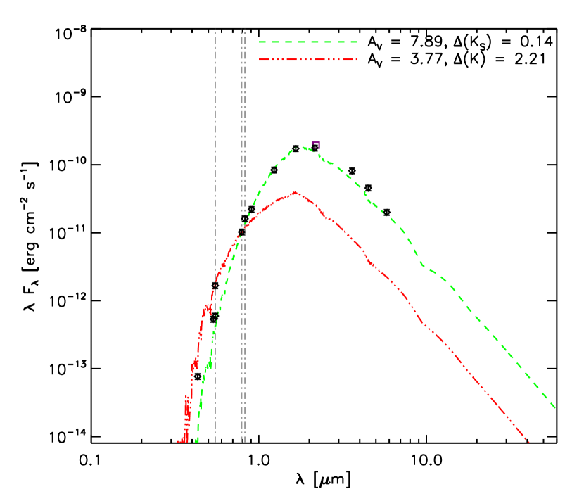
Figure 1: sed for coup 262. Diamonds are photometric data from Tables 2–3 (see §2.2). The purple square is the $K$-band flux from (Hillenbrand et al., 1998) used to calculate $\Delta K_{\rm S}$ for the red atmosphere model. The green curve is the best fitting NextGen stellar atmosphere model with $T_{\rm eff}$ set to the literature value (Table 1). The best-fit extinction, $A_{V}$, is reported upper right. The red curve represents the same stellar atmosphere model but with $A_{V}$ as previously determined by Hillenbrand (1997) based on a fit to the $V$ and $I$ fluxes only. Vertical lines indicate the wavelengths of the (from left to right) $V$ and $I_{C}$ bands used by Hillenbrand (1997) and the wfi $I$-band newly reported here. The resulting $\Delta K_{\rm S}$ color excesses for both model atmosphere fits are reported at upper right (see also Table 1). It is clear that the new fit to the full set of available photometric fluxes results in a more accurate representation of the stellar sed. Whereas this star was previously identified as possessing a very large near-ir excess, the new sed fit here indicates no significant excess.

For about half of the stars in our sample, our newly measured $A_{V}$ values agree within 99% confidence with those previously reported. For the remaining stars, the $A_{V}$ values differ significantly; the reason for this difference is illustrated in Fig. 1 for the case of star coup 262. The red model sed represents the previously reported fit of a $T_{\rm eff}=4395$ K photosphere to just the $V$ and $I_{C}$ band fluxes from Hillenbrand (1997). The extinction that results is $A_{V}=3.77$ (see Table 1 and Hillenbrand, 1997), and as a consequence the $K$-band flux appears to be highly in excess of the photosphere with $\Delta(I-K)=2.21$ (Hillenbrand et al., 1998). However it is evident from visual inspection of the complete set of observed fluxes that this model fit is a poor representation of the additional measurements included here. As shown in the figure, our new fit to the entire set of fluxes gives $A_{V}=7.91^{+0.70}_{-0.53}$ and $\Delta K_{\rm S}$ $=0.14\pm 0.11$. For this particular case, evidently the previously reported $V$-band flux was anomalously high by $\sim 5\sigma$ (perhaps due to the ubiquitous optical variability of pms stars), and so fitting for $A_{V}$ to just the $V$ and $I_{C}$ fluxes resulted in a distorted model sed. The difference between the two sed fits is important in the context of our study: e.g., the previously reported value of $\Delta(I-K)$ for coup 262 implies a massive, warm circumstellar disk close to the star, whereas our newly determined best-fit sed model is in fact consistent with no close-in disk. We revisit the sed fit of coup 262 in the context of the entire study sample below (§§ 4 and 6).

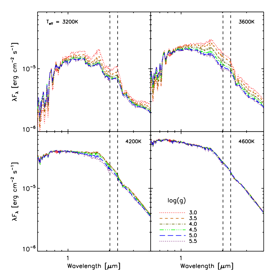
Figure 2: Effects of changing surface gravity ($\log g$) on flux in the $K_{S}$ passband (represented by vertical dashed lines) as a function of stellar temperature. Each pane represents a different temperature within the expected range for young, low-mass stars in our study sample. In each plot, solar-metallicity NextGen stellar atmospheres are plotted with six different $\log g$ values. Each atmosphere is normalized to the $I_{\rm WFI}$ bandpass at 0.83 $\mu$m, indicated by red diamonds. For cooler stars, i.e., the atmospheres in the upper panels, $K_{S}$ flux varies by a factor of three depending on $\log g$; the effect is most pronounced at $T_{\rm eff}\lesssim 4000$ K.

Hillenbrand (1997) adopted photospheric colors of main-sequence dwarfs (i.e., for dwarfs, $\log g\sim 4.5$) in the calculation of near-ir excesses. However, low-mass pms stars at the young age of the onc ($\sim 1$ Myr) are expected to have somewhat lower $\log g$ valuesdue to their large radii. Thus we have also considered the extent to which the assumed $\log g$ affects the predicted stellar colors and thus the inferred near-ir excesses. In Fig. 2, we compare the seds of NextGen stellar atmosphere models as a function of $\log g$ for several representative $T_{\rm eff}$ appropriate for our study sample (all models shown are solar metallicity). We see that the choice of $\log g$ is not important for stars warmer than $T_{\rm eff}\gtrsim 4200$ K. However, we find that for cooler objects the predicted $I-K$ colors become increasingly redder with decreasing $\log g$, which could lead to over-estimated near-ir excesses for the coolest stars. Therefore in this study we have opted to use model atmospheres with $\log g$ appropriate to each object ($\log g$ calculated from previously reported stellar masses and radii; see Table 1).

Newly determined $\Delta K_{\rm S}$ values following the procedure described above are reported in Table 1. Several previous studies (e.g., Stassun et al., 1999; Rebull, 2001; Herbst et al., 2002; Lamm et al., 2004; Makidon et al., 2004), adopted a threshold value of $\Delta K_{\rm S}$ $>0.3$ (i.e., $\sim 3\sigma$ excess given typical $\sigma_{K}=0.1$ mag; see Sec. 2.2) for identifying stars with close-in circumstellar disks. By this criterion alone, five of the stars in our sample (COUP 141, 223, 1246, 1343, 1608) show large near-ir excesses indicative of the presence of warm circumstellar dust . The remaining stars in our sample show very weak or no evidence for near-ir excess emission (i.e., $\Delta K_{\rm S}$ $<0.3$).

In the context of the principal aims of the present study—where we seek to determine whether the large magnetic loops observed in the sample stars are linked to circumstellar disks—one might anticipate that $\Delta K_{\rm S}$ could be used as a quantitative tracer of circumstellar dust located within reach of the observed magnetic loops. For example, if the presence of substantial $\Delta K_{\rm S}$ excess correlates with the location of the disk truncation radius ($R_{\rm trunc}$, the distance from the inner edge of the disk to the star), then we might simply take stars with $\Delta K_{\rm S}$ $>0.3$ as those whose inner disks are likely to be magnetically linked to the star. This is similar to the approach of Getman et al. (2008b).

The combination of factors discussed above, however—relatively cool stellar photospheres which peak in the near-ir, magnetic flaring loops that are large enough to interact with disks at relatively large heights above the stellar surface, etc.—makes near-ir excess an inefficient tracer of the types of disks we seek to characterize. Table 4 categorizes the sample stars according to whether or not they display significant near-ir excess emission (i.e., $\Delta K_{\rm S}$ $>0.3$ vs. $\Delta K_{\rm S}$ $<0.3$) and whether the inner-disk truncation radius is larger or smaller than the dust destruction radius (i.e., $R_{\rm trunc}>R_{\rm dust}$ vs. $R_{\rm trunc}\lesssim R_{\rm dust}$, where $R_{\rm dust}$ is the distance from the star within which dust is warm enough to sublimate). Here $R_{\rm trunc}$ is determined from our detailed sed model fitting as described below (§4). The off-diagonal elements of Table 4 represent cases contradicting the assumption that $\Delta K_{\rm S}$ excess correctly and quantitatively predicts the location of the inner-disk edge. For only one of the sample stars (COUP 1246) do we find a relatively large inner-disk hole ($R_{\rm trunc}>R_{\rm dust}$) but a large $\Delta K_{\rm S}$ $>0.3$. This one case appears unusual because the best-known explanation for a strong near-ir excess is the presence of warm dust close to the star. Upon closer inspection of this case (COUP 1246), we found that the fitted $A_{V}$ was underestimated because of the presence of a moderate blue excess, likely due to chromospheric activity as suggested by the observed filled-in Ca II emission (Table 1), and which is not included in the photosphere model. If we manually adjust the $A_{V}$ value upward by $\sim 3\sigma$ from the fit value of $A_{V}=1.52^{+0.70}_{-0.60}$ (see Table 1) to $A_{V}=2.22$, the value of $\Delta K_{\rm S}$ becomes 0.17. Indeed, our final best fit sed model (see §4) has an $A_{V}$ of 3.04, and thus an even lower $\Delta K_{\rm S}$. Therefore, for the following analysis and discussion, we assume that the calculated excess $\Delta K_{\rm S}$ in COUP 1246 is not significant (i.e., $\Delta K_{\rm S}$ is consistent with being less than 0.3).

Several stars in our sample exhibit a meager $\Delta K_{\rm S}$ $<0.3$, and by this criterion alone would be classified as lacking close-in, hot dust. However, for eight of these stars (in the lower left quadrant of Table 4), our sed fitting found these to in fact have disks that reach relatively close to the star ($R_{\rm trunc}\lesssim R_{\rm dust}$), and in some cases (shown below, §6), the disk reaches sufficiently close to the star to interact with the observed large flaring loops. In summary, Table 4 indicates that while $\Delta K_{\rm S}$ $\geq 0.3$ appears to be an accurate indicator of dusty material close to the star, the lack of significant $\Delta K_{\rm S}$ does not rule out the presence of dusty material close to the star. Thus, for the purposes of the present study where we seek to establish more quantitatively the location of the inner-disk edge in relation to the observed large magnetic flaring loops, we cannot rely solely on traditional near-ir excesses.

In addition to $\Delta K_{\rm S}$ measurements, from our new sed fits we calculate blueward color excesses, $\Delta(U-V)$ which can be used as a tracer of accretion at the stellar surface (“hot spots”) and/or chromospheric activity and can help in our interpretation of some seds (see §5; these are reported in Table 1.). Table 5 categorizes the sample stars in a manner similar to Table 4, but now using $\Delta(U-V)$. We identify objects with $\Delta(U-V)$ $<-0.3$ as those likely possessing hot accretion spots on their surfaces (see Rebull et al., 2000) and thus likely to be undergoing active accretion (but see Findeisen & Hillenbrand, 2010, for a discussion of other phenomena that may cause blue excesses in pms stars). Five of the sample stars show evidence for active accretion, and all but one of these have $R_{\rm trunc}\lesssim R_{\rm dust}$ as expected for a disk that extends close enough to the star for accretion to occur. Furthermore for two of these stars the Ca II measurements of Hillenbrand (1997, see Table 1) also indicate active accretion. Only one star (COUP 1568) fails to show $\Delta(U-V)$ excess despite possessing a close-in disk edge. Thus, while $\Delta(U-V)$ cannot provide a quantitative measure of the location of the inner disk for non-accretors [$\Delta(U-V)$ $>-0.3$], it is as expected a relatively reliable indicator of $R_{\rm trunc}\lesssim R_{\rm dust}$ for active accretors [$\Delta(U-V)$ $<-0.3$].

In the analysis that follows, we use detailed sed fits over the full range of available photometric data (Tables 2 and 3). Where applicable, we use the $\Delta K_{\rm S}$ and $\Delta(U-V)$ excesses and Ca II equivalent widths in Table 1 as secondary information to aid our classifications in order to characterize in detail the presence and structure of circumstellar disks in our sample.

4 SYNTHETIC SPECTRAL ENERGY DISTRIBUTION MODELS

To compare the observed seds of our sample with the seds expected from young stars with disks within reach of the observed flaring loops, we employed the Monte Carlo radiative transfer code of Whitney et al. (2003a, b), ttsre, to generate synthetic seds. Our aim is to more quantitatively constrain the structure of any circumstellar material around each of the 32 stars in our sample so that we may determine, in detail for each star, whether there is in fact disk material within reach of the magnetic loops observed by Favata et al. (2005). Thus for each of the stars in our sample, we wish to determine the range of disk parameters—the most important of these being the location of the inner edge of the disk—that are able to reproduce the observed seds (§2).

The ttsre code models randomly emitted photons from the central illuminating source and follows the photons as they interact with (i.e., are absorbed or scattered by) any circumstellar material. The circumstellar material is modeled as an optically thick dust disk extending from an inner truncation radius, $R_{\rm trunc}$, to an outer radius of typically a few hundred au. The disk in general may be “flared” such that its scale-height increases with increasing distance from the star, or it may be flat. Surrounding the star and disk may be a spherically distributed infalling envelope with bipolar cavities; such an envelope is generally required for reproducing the scattered-light properties of embedded objects (generally seen as moderate excesses in the blue; e.g., Stark et al., 2006). The code also self-consistently solves for thermal equilibrium in the disk as absorbed photons heat the disk and are re-radiated. Sublimation of dust is also included (for details of the dust properties used by the code, see Table 3 of Whitney et al., 2003b). The code models the central illuminating source using the NextGen atmosphere models of Hauschildt et al. (1999). We adopted the solar-metallicity atmosphere models, with $\log g$ and $T_{\rm eff}$ chosen according to each star’s observationally determined $M_{\rm star}$, $R_{\rm star}$, and $T_{\rm eff}$ (Table 1).

Because of the very large number of permutations on the possible star/disk/envelope parameters included in the ttsre model (i.e., disk mass, disk inner and outer radius, disk flaring profile, disk accretion rate, disk inclination angle, etc.), there is in general not a simple one-to-one correspondence between a given observed sed and, say, $R_{\rm trunc}$. Thus, to fully explore the range of disk parameters that could possibly reproduce the observed seds of our sample, we made use of the very large grid of ttsre models constructed by Robitaille et al. (2006). The grid includes some 200,000 models representing 14 star/disk/envelope parameters (see Table 1 of Robitaille et al., 2006) that were independently varied to encompass virtually all possible combinations for young stellar objects with masses 0.1–50 M_⊙ in the Class 0–iii stages of evolution. The parameter space for this grid was specifically set to be very finely sampled for T Tauri stars (i.e., $T_{\rm eff}<$5200 K); at higher temperatures, $\gtrsim$5200 K, the grid is more sparsely sampled. Whereas at $T_{\rm eff}<$5200 K the grid is sampled in $R_{\rm trunc}$ by $\sim$5%, at $T_{\rm eff}>$ 5200 K it is sampled much more sparsely at $\sim$50%. This issue affected only the hottest object in our sample, coup 597 (see §5.1). Additionally, by construction, the models in this grid are set to only include non-zero accretion rates and to always include emission from a hot accretion spot on the star. As a result, in some cases blueward excess due to the hot accretion spots is seen in the best-fit model seds, which we disregard when we lack $U$ or $B$ band fluxes to constrain the blue side of the sed.

With the added free parameter of extinction, $A_{V}$, we searched the grid via $\chi^{2}$ minimization for all synthetic seds that fit the observed sed of a given star within the 99% confidence level (that is, we rejected those models that yielded a $\Delta\chi^{2}$ goodness-of-fit likelihood of 1% or less relative to the best-fit model; Press et al., 1995). For stars with spectral-type determinations from the literature (see Table 1), we furthermore require the model fits to have stellar $T_{\rm eff}$ within 500 K of the literature value except for a few cases where we found it necessary to relax the $T_{\rm eff}$ constraint in order to achieve an acceptable sed fit; these exceptions are noted when we discuss each object individually below.

In addition to temperature, we also filter the best-fit models by disk mass. In fitting the seds of the sample stars, particularly in cases with little or no ir excess emission in the observed sed, we found that a number of the best-fit models nonetheless had disks with small R_trunc, but only if the disk also had a very low mass. The extensive model grid of Robitaille et al. (2006) allows for disks with masses as low as $10^{-10}\;{\rm M}_{\odot}$. Such low disk masses, however, may be well below what is physically realistic, and certainly below what is observable, for young T Tauri stars. Recent detailed studies of pms stars with so-called “transitional” and “pre-transitional” circumstellar disks (e.g., Espaillat et al., 2007)—disks that are undergoing the rapid disk-clearing process from the inside out (e.g., Barsony et al., 2005)—show that even at this late stage the circumstellar disks are in fact quite massive. For example, Espaillat et al. (2007) derive $M_{\rm disk}\approx 10^{-1}$ M_⊙ for the pre-transitional disk of LkCa 15 with $R_{\rm trunc}\sim 45$ au, and $M_{\rm disk}\approx 10^{-2}$ M_⊙ for the slightly more evolved disk of UX Tau A, with $R_{\rm trunc}\sim 60$ au. A more extreme case is that of CoKu/Tau 4, for which D’Alessio et al. (2005) find an extremely low $M_{\rm disk}\approx 10^{-3}$ M_⊙. In what follows, we will thus restrict our analysis to include only model seds with $M_{\rm disk}>10^{-3}$ M_⊙ as more accurately representing the empirical disks of young, low-mass stars. For illustrative purposes, however, we display all models with disk masses greater than 10^-4 M_⊙.

In addition, for the purpose of interpreting the resulting best-fit model seds, we found it useful for each star to generate an additional ttsre synthetic sed as a fiducial reference model. For the cases where there is apparent ir excess in the data indicating the presence of a disk, we generate a fiducial model identical to the best-fit sed model, except that we set $R_{\rm trunc}$ equal to the magnetic loop height, $R_{\rm loop}$ (Table 1). In the cases for which the data show no ir evidence for dusty disks, the fluxes of the best fit sed model are essentially arbitrary beyond the longest wavelength data point. For simplicity in these cases our fiducial model is a simple star$+$disk sed, adopting stellar properties from the literature. The modeled structure is that of an optically thick, geometrically thin, slightly flared disk with no envelope and no accretion. The disk mass in these cases is set to 0.01 M_☉, and its inner truncation radius is again set equal to the magnetic loop height. Thus, in all cases, the fiducial model allows a direct, visual comparison of the observed and best-fit seds against that expected if the inner disk is within reach of the magnetic flaring loop. It is important to note that in cases where the magnetic loop height is within the dust destruction radius, the disk is truncated at dust destruction by default (i.e., the ttsre models require $R_{\rm trunc}\geq R_{\rm dust}$).

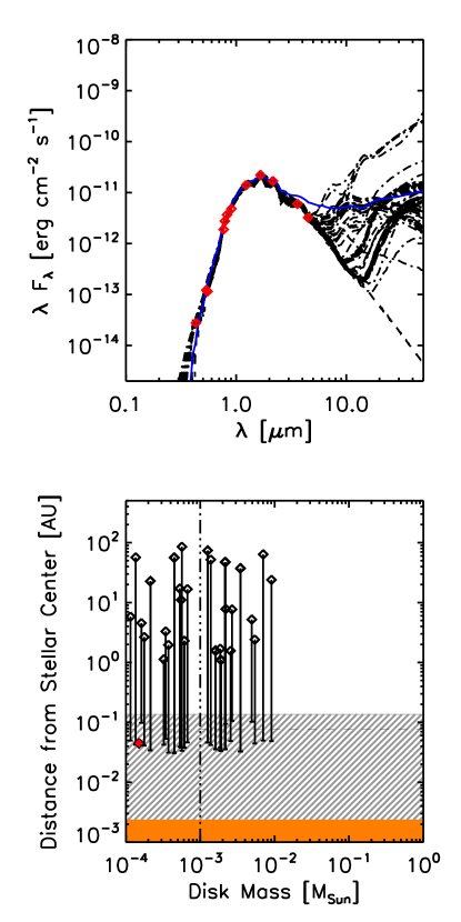
Figure 3: sed of coup 1410, category 3. All models are consistent with category 3; the SED is consistent with a bare photosphere. This object is discussed in greater detail in $\S$5.2. Upper panel: Best fit model seds from the model grid of Robitaille et al. (2007, black dash-dotted curves). The fiducial ttsre model with $R_{\rm trunc}=R_{\rm loop}$ (see §4), shown as a solid blue line and normalized to the peak near-ir flux ($J$, $H$, or $K_{S}$ band), is meant to illustrate approximately how the sed would appear if there were a disk within reach of the flaring magnetic loop. The dashed curve is a solar-metallicity NextGen atmosphere model representing the stellar photosphere. Red diamonds are measured fluxes (Tables 2–3) as detailed in §2.2. Lower panel: Comparison of $R_{\rm loop}$ and $R_{\rm trunc}$ for best-fit sed models. A dashed line illustrates the loop height above the stellar surface (solid, orange). Uncertainty in the loop height is shown as a gray, hatched region. Open diamonds represent the $R_{\rm trunc}$ values of the best-fit sed models from the upper panel. For each model, a vertical bar indicates the location of $R_{\rm dust}$ for that model (according to Eq. 1). Filled red diamonds indicate models which have $R_{\rm trunc}\approx R_{\rm dust}$ (see $\S$5 for more detail). Finally, the vertical dash-dotted line indicates our disk mass threshold value, 10^-3 M_⊙; less massive disks do not represent the disks typical of T Tauri stars (see §4). Figures for all 32 sample stars are available in color electronically (Figs. 3.1-3.32).

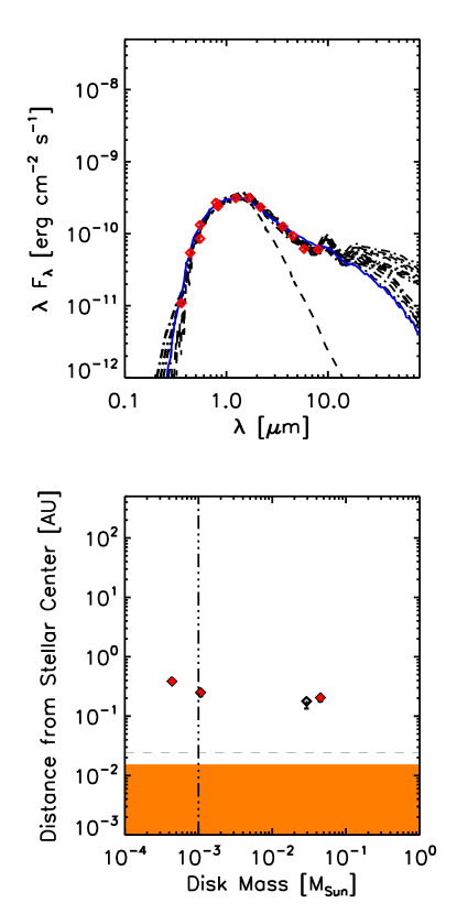
Figure 4: sed of coup 141, category 2. All symbols are as in Fig. 3. 2/3 models are consistent with category 2. Excess flux in the irac bands indicates a dusty disk. Fourteen best-fit seds are plotted, but three of these are degenerate in $M_{\rm disk}$ or $R_{\rm trunc}$, representing four inclinations of the same star–disk configuration. Three sets of model seds have $M_{\rm disk}>10^{-3}$ M_☉, and more than 2/3 of these are truncated at their respective dust destruction radii (red points in lower panel). Thus these disks may possess gas that extends inward of $R_{\rm dust}$ to $R_{\rm loop}$. This object is very likely accreting, based on its strong Ca II emission ($-$17.8Å) and $\Delta(U-V)$ excess of $-1.26$. For further discussion of this object, see $\S$5.2.

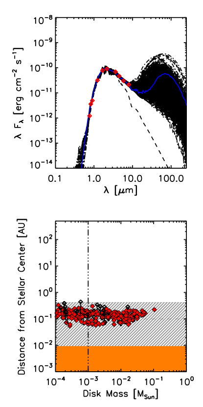
Figure 5: sed of coup 720, category 1. All symbols are as in Fig. 3. All 175 models are consistent with category 1. This object is discussed in detail in §5.2.

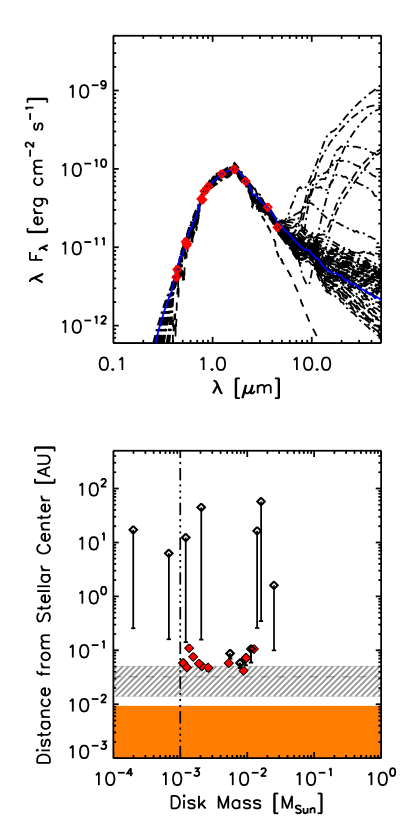
Figure 6: sed of coup 997, category 4. All symbols are as in Fig. 3. Most of the best fit model results are split between categories 2 (11/20) and 3 (9/20), placing this object into category 4. This object is discussed in detail in §5.2.

We present in this work the seds of the 32 stars in our study sample. Flux measurements and upper limits (Tables 2–3) are represented by diamond symbols with error bars (which are in most cases smaller than the symbols) and blue triangles, respectively. The sed of the underlying stellar photosphere (NextGen atmosphere) is shown for comparison as a dashed line. Superposed on the observed seds, the best-fitting sed models from the grid of Robitaille et al. (2006) discussed above are shown as dash-dotted curves. The fiducial ttsre model that we calculated is shown as a solid, blue curve. Figures 3–6 are included in print for illustrative purposes below (see §5), with the remaining figures accessible electronically.

5 INTERPRETING THE SPECTRAL ENERGY DISTRIBUTIONS

With observed and model seds in hand for all 32 stars in our study sample, we can now attempt to answer the central question of this paper: Are the large flaring loops observed on these stars likely due to a magnetic star-disk interaction, or do they represent primarily stellar phenomena unrelated to disks? To answer this question, in this section we discuss the specific criteria by which we determine, from examination of each star’s sed, the likelihood that it possesses a disk whose inner edge is within reach of the observed flaring magnetic loop.

5.1 sed Categorization Criteria

As discussed above, in general we found that $R_{\rm trunc}$ correlates with $M_{\rm disk}$ in the model seds, e.g., a small $R_{\rm trunc}$ can fit even a bare photosphere sed if $M_{\rm disk}$ is made sufficiently small (see §4). Thus we found it helpful to visualize $R_{\rm trunc}$ versus $M_{\rm disk}$, as shown in the lower panel of Figs. 3–6 in order to better interpret the sed model fits. A vertical line at 10^-3 M_⊙ indicates our disk mass threshold (see §4). In orange, we show the stellar photosphere for reference. In each figure, the $M_{\rm disk}$ and $R_{\rm disk}$ values corresponding to each model sed from the upper panel are shown as diamonds. For comparison, the magnetic loop height ($R_{\rm loop}$) and its uncertainty (see §2.1) are shown as a dashed line and a hatched region, respectively.

From these plots, we can thus begin to assess the degree of spatial correspondence between $R_{\rm trunc}$ and $R_{\rm loop}$ for each star. Cases for which $R_{\rm trunc}\leq R_{\rm loop}$ can be interpreted as representing disks that are within reach of the observed flaring loops. Cases for which $R_{\rm trunc}>R_{\rm loop}$ are somewhat less straightforward to interpret because we must first account for the effects of dust sublimation. The location of dust destruction, or the sublimation radius, is calculated using each model’s stellar temperature and radius as follows (Robitaille et al., 2006):

$$R_{\rm dust}=R_{\rm star}\times\left(\frac{1600~{}{\rm K}}{T_{\rm star}}\right)^{-2.1}$$ (1)

where 1600 K is the dust sublimation temperature. Uncertainties in $R_{\rm star}$ and $T_{\rm star}$ create a range of possible values for $R_{\rm dust}$. We adopt 5% uncertainty in $T_{\rm star}$ and 20% uncertainty in $R_{\rm star}$ in this calculation (see e.g., Hillenbrand, 1997). In each of Figs. 3–6 (and in figures 3.1-3.32, accessible online), filled (red) diamonds represent models effectively truncated at the dust destruction radius, $R_{\rm dust}$, while unfilled points have vertical bars in the $-y$ direction to show where that particular model’s dust destruction radius is located. For the model uncertainty in $R_{\rm trunc}$, we adopt 5% and 50% for stars with $T_{\rm eff}<$5200 K and $T_{\rm eff}>$5200 K, respectively (see §4). Thus, when we say the disk is truncated “effectively” at the dust destruction radius, the intended meaning is that $R_{\rm trunc}$ and $R_{\rm dust}$ are equivalent within their uncertainties. We also report fiducial $R_{\rm dust}$ values for our sample stars in Table 1; these are calculated using Eq. 1 and the $R_{\rm star}$ and $T_{\rm star}$ data in that same table.

The broadband fluxes used here trace the spatial extent of a disk’s dust; in principle the inner edge of the gas in the disk could extend even closer to the stellar surface. For the cases in which we find that an observed dust disk is truncated at the dust destruction radius, the dust disk is likely truncated by sublimation, a process which would not remove gas. Indeed, some systems have been observed to be accreting even though the dust disk is truncated far from the star (Eisner et al., 2005, 2007). For dust disks truncated near the sublimation radius, but not within reach of the magnetic loop, it is possible that a gas disk extends closer to the star and is truncated within the loop height (this has been observed by Najita et al., 2003; Eisner et al., 2005). Conversely, if the dust disk is truncated outside the dust destruction radius, some other process may be responsible for clearing out the inner portion of the disk, and therefore we assume that the inner gas is cleared out as well (e.g., Isella et al., 2009).

Finally, for a few stars we lack sufficient photometric data to adequately constrain the location of $R_{\rm trunc}$. In most cases, this is due to a lack of Spitzer photometry and thus the longest wavelength measurement is the 2mass 2.2 $\mu$m flux. Consequently, the model seds in these cases are largely unconstrained and result in a wide variety of possible star-disk configurations which can fit the observed sed.

Based on these considerations, in what follows we categorize our sample stars into four groups, based on the degree to which the seds indicate that the inner disk edge is within reach of the flare loop height:

Category 1:

$R_{\rm trunc}\leq R_{\rm loop}$: The inner disk edge is clearly within reach of the magnetic flaring loop.

Category 2:

$R_{\rm trunc}>R_{\rm loop}$ but $R_{\rm trunc}\approx R_{\rm dust}$: The dusty inner disk edge is beyond the flaring loop height, however the dust disk is truncated at the dust-destruction distance and thus a gas disk may extend inward to $R_{\rm loop}$ (i.e., $R_{\rm trunc}\lesssim R_{\rm dust}$).

Category 3:

$R_{\rm trunc}>R_{\rm loop}$ and $R_{\rm trunc}>R_{\rm dust}$: The inner edge of the dust disk is clearly beyond reach of the magnetic flaring loop.

Category 4:

Indeterminate: More than one category above is permitted by the available data (generally due to lack of Spitzer data).

Recall that we take half the loop length as the flare loop height, as a conservative upper limit (see §2.1). In general, for a given star there are multiple sed models that are good fits to the observed sed, and in some cases the multiple best-fitting model seds yield a mixed verdict regarding the placement of $R_{\rm trunc}$ with respect to $R_{\rm loop}$. Thus if one of categories 1–3 above is favored by more than $\frac{2}{3}$ of the best-fit sed models, we assign the star to that category, and we assign “indeterminate” (category 4) otherwise.

5.2 Example Cases

As an example of our approach to interpreting the seds of our study sample, we show in Fig. 3 (upper panel) the sed of coup 1410. The fiducial sed model in Fig. 3, corresponding to a disk with $R_{\rm trunc}=R_{\rm loop}$, predicts an excess of ir flux at wavelengths as short as 3 $\mu$m, unlike the data and best-fit model seds which follow the profile of a bare stellar photosphere to 4.5 $\mu$m. Intuitively, this implies that the best-fit model seds must therefore correspond to disks with moderately large inner holes. Indeed, the lower panel of Fig. 3 shows that nearly all of the best-fit model seds, representing disks with $10^{-4}\lesssim M_{\rm disk}/{\rm M}_{\odot}\lesssim 10^{-2}$, have $R_{\rm trunc}>1$ au. Furthermore, the majority of these models are truncated well outside their respective dust destruction radii (i.e., $R_{\rm trunc}>R_{\rm dust}$); only one fit model has $R_{\rm trunc}\lesssim R_{\rm dust}$, and this model has very low $M_{\rm disk}$, below our threshold of 10^-3 M_⊙

Note that the observed sed for this star does not in fact require any disk at all; the fact that many of the sed models shown in Fig. 3 exhibit large excesses longward of 4.5 $\mu$m implies only that these hypothetical disks with very large inner holes are formally permitted by the available data. These models thus provide a lower limit to the size of $R_{\rm trunc}$ that any as-yet undetected disk could possibly have. Since this lower limit is in this case much larger than $R_{\rm loop}$, we conclude that no disk is present that could interact with the observed magnetic flaring loop, and we assign coup 1410 to category 3 ($\S$5.1).

coup 141 (Fig. 4) is a case in which the observed sed is reasonably well matched by the fiducial sed model, for which $R_{\rm trunc}=R_{\rm loop}$. The best-fit seds have inner truncation radii well beyond reach of the magnetic loop. However, these models’ inner disk radii are also equal to their dust destruction radii, and thus it is likely that sublimation is responsible for the apparent clearing of the inner disk. In cases like coup 141, while the magnetic loop may not intersect the dust disk, it could nonetheless intersect a gas disk that extends inward of the dust to within reach of $R_{\rm loop}$. Indeed, both Ca II and $\Delta(U-V)$ strongly indicate active accretion (Table 1). Thus we assign coup 141 to category 2.

As another example, consider coup 720 (Fig. 5). In this case, all of the best-fit model seds with $M_{\rm disk}$ above our adopted threshold of 10^-3 M_⊙ have similar $R_{\rm trunc}\sim 0.1$ au, which overlaps $R_{\rm loop}$ within its uncertainty. Many of these best-fit models, moreover, have $R_{\rm trunc}\approx R_{\rm dust}$, and thus may possess gas disks that extend even closer to the star. coup 720 thus represents a good example of an sed that is consistent with $R_{\rm trunc}\approx R_{\rm loop}$, and for which the large magnetic loops observed by coup may facilitate the magnetic star-disk interaction envisaged in magnetospheric accretion models. coup 720 is assigned to category 1.

Finally, consider coup 997 (Fig. 6). The observed sed data (0.34–4.5 $\mu$m) show excess ir flux. About half of the best-fit models are truncated at their dust destruction radii (category 2), while the other half are truncated beyond 1 au (category 3). We also do not have Ca II or $\Delta(U-V)$ measurements to help disambiguate the two possibilities, and thus it is not possible to say which set of models correctly describes the observed star-disk system. Requiring additional data (particularly longward of $\sim 10\mu$m) to discriminate between the category 2 and 3 model fits, we assign this object to category 4.

6 RESULTS

In Table 6, we present a summary of the results for the 32 stars in our sample. Following the procedure described in §5, we have identified which stars’ seds have massive (i.e., $\geq$10^-3M_⊙) disks that are consistent with being within reach of the observed magnetic loops. Notes about each star relevant to its classification are provided in the figure captions.

We find six stars that appear to have seds consistent with $R_{\rm trunc}\leq R_{\rm loop}$ (category 1). Another four stars do not show direct evidence of disks within reach of the magnetic loops, but could potentially have gas that extends interior to the observed dusty inner edge of the disk (category 2). Fourteen stars either have disks whose inner edges are situated beyond the reach of the magnetic loops, or are simply devoid of detected disk material entirely (category 3). For eight stars, we could not assign a definitive category as additional data are necessary to support or eliminate different classes of best-fit sed models (category 4).

7 DISCUSSION AND CONCLUSIONS

Of the 24 stars in our 32-star sample for which we have enough optical–infrared data to constrain the location of the disk inner edge (i.e., excluding stars in category 4; §5.1 and Table 6), for about 58% we are able to rule out close-in, massive disks within reach of the observed large flaring loops (category 3). These energetic flares discovered by Favata et al. (2005) are evidently intrinsically stellar phenomena. This gives added justification a posteriori for the application of the solar-flare cooling loop model to these stars (§2.1), and suggests that it may be possible by further extension of the solar analogy to infer other flare-related properties for these flares, such as coronal heating rates and coronal mass ejections. The latter in particular may be important for furthering our understanding of mass and angular momentum loss in these low-mass pms stars.

Our sample also includes six cases for which the sed clearly indicates a dusty disk that extends close enough to the star to permit interaction with the flaring loop (category 1; Table 6). In four additional cases the dust disk appears to be truncated beyond the reach of the flaring loop, but at or close to the predicted dust destruction radius (category 2). In these cases, the dust disk may in fact be truncated by dust sublimation, a process which does not remove gas. Thus, in category 2 objects, it seems likely that a gas disk (undetected in the broadband flux measurements used in our sed models) extends closer to the star and may be within reach of the observed flaring loops. One of the four category 2 objects has a Ca II measurement from the literature (coup 141), and two have $\Delta(U-V)$ measurements (coup 141 and coup 1568). coup 141 is, interestingly, the most strongly accreting object in the sample as probed by its Ca II equivalent width (see Table 1) and it also has a very negative $\Delta(U-V)$; the combination of these indicators is strong evidence for ongoing accretion. For coup 141 the $\Delta K_{\rm S}$ near-ir excesses also indicates a disk very close to the star (see Sec. 3 and Table 4). These examples further strengthen the interpretation of the category 2 stars as likely having gas accretion disks within reach of the stellar magnetosphere.

Several studies clearly find a high frequency of close-in, massive dusty disks in the onc population as a whole. For example, Hillenbrand et al. (1998) find a disk fraction in the onc of $\sim$70% on the basis of excess emission at 2.2 $\mu$m. Thus, the $\sim$25% (category 1) or $\sim$38% (categories 1 and 2) frequency of close-in disks in our 32-star sample, representing the $\sim$1% of onc stars with the most powerful X-ray flares observed by COUP, is evidently not representative of the disk characteristics of the onc as a whole.

The six cases in which we have observed stars with close-in, dusty disks which intersect the magnetic loops (category 1) are interesting candidates for further study. Specifically, it would be informative to determine if the flares in these cases are in some way different than the category 3 cases. Three of these objects have $\Delta(U-V)$ measurements, all of them $\leq-0.3$ (Table 1), strongly indicating active accretion. Temporally linking accretion as seen in optical variability to the X-ray flare events (e.g., Stassun et al., 2006) could solidify whether a magnetic star-disk interaction has taken place. Geometric information would be necessary to determine where the magnetic loop is on the stellar surface—for example, a given flaring loop could extend in a direction perpendicular to the disk and thus not interact, even if the dust (or gas) disk is within the appropriate distance from the stellar surface.

The question of how the large magnetic structures are stabilized (prior to the flaring event) was posed in the discovery publication of these objects (Favata et al., 2005). It was proposed that the loops may be anchored to corotating disk material and thereby not subject to shear which could disrupt the loops. In this work we have found such disk-anchoring to indeed be a possibility for 10 objects (categories 1 and 2), but further analysis is needed to determine how massive and ionized a disk must be to enable interaction. For fourteen objects (category 3), disk-supported loops are unlikely, as these stars lack massive disks within reach of the loops. We speculate that as long as the confining magnetic field at the upper end of the loop is sufficiently strong and the confined material corotating, stability is feasible even without a disk. For example, Cranmer (2009) describes a loop geometry in which the pressure of the confined gas decreases with increasing loop length, implying that in fact the largest coronal loops may be most stable against rupture. Additionally, our findings may imply that the largest flaring loops cannot readily form in the presence of a disk, given that they appear in our sample to preferentially occur on stars lacking close-in disk material.

Alternate scenarios to explain the long x-ray decay timescales include observations of corotating, embedded structures in coronae (e.g., Collier Cameron & Robinson, 1989a, b), and prominences and stellar winds (Skelly et al., 2008; Massi et al., 2008). The observed coronal structures from those studies lend additional support to the idea of these large magnetic structures remaining stable in hot coronae or within the stellar wind over multiple rotation periods as the x-ray flare decays, even if no disk is present to anchor the magnetic loop (Jardine & van Ballegooijen, 2005).

In summary, the 32 most powerful flares observed by the coup survey were found to have magnetic structures multiple stellar radii in arc length confining the x-ray emitting, heated plasma (Favata et al., 2005). With the goal of understanding the nature of these large x-ray emitting flare structures, we have modeled the optical–infrared seds of these objects, finding 58% to be lacking close-in circumstellar disks to which these loops could anchor. It is evident that in at least these cases the large-scale flares are phenomena of purely stellar origin, neither triggered nor stabilized by star-disk interactions.

Table 1: Stellar Parameters

Object	Teff	Mass	Radius	Magnetic Loop	Dust Destruction	Ca II EW	Literature	Re-calculated	$\Delta(K_{S})$	$\Delta(U-V)$
Name	[K]	[M☉]	[R☉]	Height [R☉]	Radius [R☉]	[Å]	AV [mag]	AV [mag]	[mag]	[mag]
coup 7	4581	2.12	6.23	0.65	56.8	$\cdots$	0.75	0.67 (-0.58, +0.54)	0.12	0.03
coup 28	3802	0.53	2.3	7.91$\pm$5.46	14.2	1.6	0.63	0.30 (-0.30, +0.54)	0.20	0.24
coup 43	3606	0.4	2.92	16.1 (+3.16,-5.32)	16.0	1.4	1.36	1.18 (-0.60, +0.56)	0.012	0.64
coup 90	3802	0.52	2.51	1.04 (+4.86,-1.04)	15.5	1.6	4.97	3.97 (-1.13, +1.13)	0.053	$\cdots$
coup 141	5236	2.11	3.3	1.97	39.2	-17.8	1.83	2.17 (-0.63, +0.60)	0.37	-0.67
coup 223	4395	1.19	2.79	6.95	23.3	1.7	4.66	5.81 (-0.75, +0.88)	0.31	$\cdots$
coup 262	4395	1.13	1.58	28.5 (+16.8,-22.3)	13.2	2.3	3.77	7.89 (-1.20, +1.24)	0.14	$\cdots$
coup 332	3111†	0.5‡	2‡	105$\pm$38.4	8.09	$\cdots$	$\cdots$	12.8 (-1.67, +2.14)	0.032	$\cdots$
coup 342	4729†	0.5‡	2‡	20.3 (+21.4,-20.3)	19.5	$\cdots$	$\cdots$	7.89 (-0.78, +0.85)	0.085	$\cdots$
coup 454	4775	2.35	4.58	46.4 (+14.8,-9.20)	45.5	2.1	5.85	6.39 (-0.85, +0.87)	0.077	$\cdots$
coup 597	5662	1.49	2.01	3.16 (+7.62,-3.16)	28.6	4.5	2.69	3.32 (-1.35, +1.39)	0.27	-0.26
coup 649	3589	0.4	2.17	9.20	11.8	0	4.11	3.82 (-0.73, +0.83)	0.17	$\cdots$
coup 669	4581	1.52	2.59	13.2 (+2.73,-3.31)	23.6	$\cdots$	1.96	2.33 (-1.10, +1.20)	0.049	$\cdots$
coup 720	4452†	0.5‡	2‡	19.0 (+69.3,-19.0)	17.2	$\cdots$	$\cdots$	11.8 (-1.33, +1.66)	-0.23	$\cdots$
coup 752	3802	0.54	1.67	9.35 (+1.29,-9.35)	10.3	1.1	0.07	0.64 (-0.64, +1.10)	0.047	-0.70
coup 848	3342	0.29	1.98	23.3 (+4.03,-3.31)	9.31	0	1.72	1.35 (-1.34, +1.46)	0.093	$\cdots$
coup 891	4775	2.43	4.85	24.9 (+3.88,-3.31)	48.8	1.8	8.00	10.7 (-1.02, +1.12)	0.13	$\cdots$
coup 915	4613†	0.5‡	2‡	11.2 (+3.88,-2.59)	18.4	$\cdots$	$\cdots$	15.8 (-1.76, +2.56)	-0.065	$\cdots$
coup 960	3177	0.24	2.16	0.53 (+1.48,-0.53)	9.27	0	2.72	1.29 (-0.41, +0.43)	-0.013	$\cdots$
coup 971	3999	0.69	3.28	5.03 (+0.72,-0.43)	22.5	1.8	0.	0.00 (-0.00, +0.15)	-0.24	-0.80
coup 976	3177	0.18	0.91	10.9	3.85	0	0.	2.88 (-0.69, +1.13)	0.28	$\cdots$
coup 997	3856†	0.5‡	2‡	4.89 (+4.03,-3.88)	12.7	$\cdots$	$\cdots$	1.82 (-1.14, +1.13)	0.060	$\cdots$
coup 1040	4281†	0.5‡	2‡	1.25 (+1.91,-1.25)	15.8	$\cdots$	$\cdots$	16.5 (-2.03, +3.53)	-0.10	$\cdots$
coup 1083	4698†	0.5‡	2‡	33.8 (+9.63,-7.05)	19.2	$\cdots$	$\cdots$	4.16 (-0.56, +0.61)	-0.0072	$\cdots$
coup 1114	4903†	0.5‡	2‡	9.78 (+2.30,-9.78)	21.0	-1.5	$\cdots$	6.08 (-0.71, +0.74)	0.086	$\cdots$
coup 1246	3177	0.23	1.62	5.75 (+1.01,-1.15)	6.95	0	0.92	1.52 (-0.60, +0.70)	0.45	$\cdots$
coup 1343	3649†	0.5‡	2‡	13.8 (+2.45,-2.44)	11.6	$\cdots$	$\cdots$	3.04 (-0.83, +3.66)	0.60	$\cdots$
coup 1384	3802	0.52	2.46	7.33$\pm$4.46	15.1	1.9	0.	0.67 (-0.67, +0.82)	-0.095	-0.35
coup 1410	3606	0.36	0.51	15.8 (+12.9,-15.8)	2.80	0	0.57	4.98 (-0.98, +0.97)	0.053	$\cdots$
coup 1443	5528†	0.5‡	2‡	3.74 (+4.17,-0.57)	13.6	$\cdots$	$\cdots$	0.26 (-0.26, +0.55)	0.18	0.14
coup 1568	5236	2.55	3.99	0.53 (+1.62,-0.53)	48.1	$\cdots$	0.59	1.06 (-0.56, +0.60)	-0.040	-0.22
coup 1608	3724	0.48	1.76	11.8 (+2.44,-11.8)	10.8	-1.3	0.93	0.25 (-0.25, +0.41)	0.43	-1.2

Note. — $\dagger$ Temperatures not in literature; assigned T_eff from best fit SED model. $\ddagger$ Fiducial masses and radii of 0.5 M_☉ and 2 R_☉ taken in cases for which there were no measurements available in the literature.

Table 2: Hubble ACS and WFI Fluxes

Object	4317Å	5359Å	6584Å	7693Å	9055Å	0.36$\mu$m	0.44$\mu$m	0.55$\mu$m	0.83$\mu$m
Name	Flux [mJy]	Flux [mJy]	Flux [mJy]	Flux [mJy]	Flux [mJy]	Flux [mJy]	Flux [mJy]	Flux [mJy]	Flux [mJy]
coup 7	$\cdots$	$\cdots$	170	$\cdots$	$\cdots$	3.9$\pm$0.36	40.$\pm$3.7	83.0$\pm$7.6	290$\pm$27
coup 28	0.89$\pm$0.082	2.9$\pm$0.27	7.3	$\cdots$	$\cdots$	0.099$\pm$0.0091	1.1$\pm$0.10	2.7$\pm$0.25	16$\pm$1.5
coup 43	0.40$\pm$0.037	1.6$\pm$0.15	5.2	10.$\pm$0.95	20.$\pm$1.9	0.033$\pm$0.0031	0.42$\pm$0.039	1.2$\pm$0.11	15$\pm$1.4
coup 90	0.028$\pm$0.0026	0.15$\pm$0.014	0.69	1.7$\pm$0.15	4.0$\pm$0.37	$\cdots$	0.038$\pm$0.0035	0.13$\pm$0.012	2.9$\pm$0.26
coup 141	7.9$\pm$0.73	16$\pm$1.4	$\cdots$	$\cdots$	$\cdots$	1.3$\pm$0.12	$\cdots$	$\cdots$	66$\pm$6.1
coup 223	0.074$\pm$0.0068	0.32$\pm$0.029	1.6	$\cdots$	$\cdots$	$\cdots$	0.095$\pm$0.0088	$\cdots$	6.2$\pm$0.57
coup 262	0.011$\pm$0.0010	0.095$\pm$0.0088	0.57	2.0$\pm$0.18	6.7$\pm$0.61	$\cdots$	$\cdots$	0.11$\pm$0.010	4.4$\pm$0.41
coup 332	$\cdots$	$\cdots$	$\cdots$	0.049$\pm$0.0045	0.33$\pm$0.030	$\cdots$	$\cdots$	$\cdots$	$\cdots$
coup 342	0.008$\pm$0.00072	0.078$\pm$0.0072	0.52	1.9$\pm$0.17	6.3$\pm$0.58	$\cdots$	$\cdots$	0.099$\pm$0.0091	4.4$\pm$0.41
coup 454	0.11$\pm$0.010	0.64$\pm$0.059	2.6	6.8$\pm$0.62	16$\pm$1.5	$\cdots$	0.16$\pm$0.014	0.63$\pm$0.058	13$\pm$1.2
coup 597	2.0$\pm$0.18	5.8$\pm$0.54	$\cdots$	$\cdots$	26$\pm$2.4	0.34$\pm$0.032	2.3$\pm$0.22	5.3$\pm$0.48	23$\pm$2.1
coup 649	0.019$\pm$0.0017	0.10$\pm$0.0093	0.38	1.5$\pm$0.14	3.4$\pm$0.31	$\cdots$	$\cdots$	$\cdots$	2.7$\pm$0.25
coup 669	1.8$\pm$0.17	6.6$\pm$0.61	15	$\cdots$	$\cdots$	$\cdots$	2.4$\pm$0.22	5.6$\pm$0.52	31$\pm$2.8
coup 720	$\cdots$	$\cdots$	0.070	0.31$\pm$0.029	1.5$\pm$0.14	$\cdots$	$\cdots$	$\cdots$	0.99$\pm$0.091
coup 752	0.85$\pm$0.078	2.6$\pm$0.24	7.1	10.$\pm$0.92	16$\pm$1.4	0.18$\pm$0.016	1.3$\pm$0.12	3.0$\pm$0.27	16$\pm$1.5
coup 848	0.097$\pm$0.0089	0.37$\pm$0.034	1.5	3.3$\pm$0.30	6.9$\pm$0.63	$\cdots$	$\cdots$	0.46$\pm$0.042	5.4$\pm$0.50
coup 891	0.002$\pm$0.00022	0.046$\pm$0.0043	0.40	2.1$\pm$0.20	9.1$\pm$0.84	$\cdots$	$\cdots$	0.046$\pm$0.0042	5.7$\pm$0.53
coup 915	$\cdots$	$\cdots$	$\cdots$	$\cdots$	$\cdots$	$\cdots$	$\cdots$	$\cdots$	0.17$\pm$0.015
coup 960	0.022$\pm$0.0020	0.082$\pm$0.0075	0.40	1.6$\pm$0.14	4.3$\pm$0.40	$\cdots$	0.029$\pm$0.0027	0.076$\pm$0.0070	3.1$\pm$0.28
coup 971	10.$\pm$0.96	21$\pm$2.0	43	$\cdots$	$\cdots$	1.6$\pm$0.15	11$\pm$1.0	$\cdots$	64$\pm$5.9
coup 976	0.016$\pm$0.0015	0.080$\pm$0.0074	0.51	1.4$\pm$0.13	3.8$\pm$0.35	$\cdots$	$\cdots$	$\cdots$	2.7$\pm$0.25
coup 997	0.60$\pm$0.055	2.1$\pm$0.19	5.9	11$\pm$0.98	18$\pm$1.7	$\cdots$	0.77$\pm$0.071	2.0$\pm$0.18	14$\pm$1.3
coup 1040	$\cdots$	$\cdots$	$\cdots$	$\cdots$	$\cdots$	$\cdots$	$\cdots$	$\cdots$	0.10$\pm$0.0093
coup 1083	0.43$\pm$0.040	1.8$\pm$0.17	6.2	14$\pm$1.3	26$\pm$2.4	$\cdots$	0.55$\pm$0.051	1.7$\pm$0.16	18$\pm$1.7
coup 1114	0.23$\pm$0.021	1.6$\pm$0.15	7.0	$\cdots$	$\cdots$	$\cdots$	0.38$\pm$0.035	1.6$\pm$0.14	37$\pm$3.4
coup 1246	0.046$\pm$0.0043	0.22$\pm$0.020	1.2	1.3$\pm$0.12	5.2$\pm$0.48	$\cdots$	0.059$\pm$0.0055	0.19$\pm$0.017	3.9$\pm$0.36
coup 1343	0.058$\pm$0.0054	0.31$\pm$0.028	1.7	2.8$\pm$0.26	6.7$\pm$0.62	$\cdots$	0.082$\pm$0.0075	0.27$\pm$0.025	5.0$\pm$0.46
coup 1384	2.8$\pm$0.26	7.9$\pm$0.73	17	$\cdots$	$\cdots$	0.39$\pm$0.036	3.3$\pm$0.30	6.9$\pm$0.64	30.$\pm$2.7
coup 1410	0.0040$\pm$0.00037	0.022$\pm$0.0020	0.13	0.48$\pm$0.045	1.4$\pm$0.13	$\cdots$	$\cdots$	0.021$\pm$0.0019	1.0$\pm$0.093
coup 1440	1.9$\pm$0.18	6.2$\pm$0.57	15	$\cdots$	24$\pm$2.2	0.21$\pm$0.019	2.5$\pm$0.23	6.0$\pm$0.56	31$\pm$2.8
coup 1568	$\cdots$	85$\pm$7.8	$\cdots$	$\cdots$	$\cdots$	8.4$\pm$0.77	50.$\pm$4.6	$\cdots$	202$\pm$19
coup 1608	$\cdots$	1.4$\pm$0.13	$\cdots$	$\cdots$	$\cdots$	0.20$\pm$0.018	0.73$\pm$0.068	$\cdots$	11$\pm$1.02
Zero points	25.793	25.744	22.393	25.291	24.347	1823 Jy	4130 Jy	3640 Jy	2430 Jy

Note. — The first five data columns report HST fluxes, the last four columns report WFI fluxes. Zeropoint fluxes used are reported in the final row of the table.

Table 3: $V$, $I$, 2MASS, and Spitzer Fluxes

Object	0.55$\mu$m	0.79$\mu$m	1.235 $\mu$m	1.662 $\mu$m	2.159 $\mu$m	3.6 $\mu$m	4.5 $\mu$m	5.8 $\mu$m	8.0 $\mu$m	23.6 $\mu$m
Name	Flux [mJy]	Flux [mJy]	Flux [mJy]	Flux [mJy]	Flux [mJy]	Flux [mJy]	Flux [mJy]	Flux [mJy]	Flux [mJy]	Flux [mJy]
coup 7	102$\pm$9.4	280$\pm$25	460$\pm$42	590$\pm$54	440$\pm$41	200$\pm$18	130$\pm$12	84$\pm$7.8	50.$\pm$4.6	10
coup 28	3.8$\pm$0.35	17$\pm$1.6	39$\pm$3.6	47$\pm$4.4	41$\pm$3.8	20.$\pm$1.8	13$\pm$1.2	8.9$\pm$0.82	6.5$\pm$0.60	14
coup 43	2.2$\pm$0.20	15$\pm$1.4	51$\pm$4.7	72$\pm$6.6	62$\pm$5.7	33$\pm$3.0	23$\pm$2.1	16$\pm$1.4	11$\pm$0.98	$\cdots$
coup 90	0.084$\pm$0.0078	1.8$\pm$0.16	14$\pm$1.2	27$\pm$2.5	27$\pm$2.5	16$\pm$1.5	11$\pm$1.0	6.6$\pm$0.60	$\cdots$	$\cdots$
coup 141	24$\pm$2.2	71$\pm$6.6	130$\pm$12	180$\pm$16	170$\pm$16	150$\pm$14	140$\pm$13	120$\pm$11	160$\pm$15	$\cdots$
coup 223	0.42$\pm$0.038	5.1$\pm$0.47	39$\pm$3.6	93$\pm$8.6	120$\pm$11	140$\pm$13	130$\pm$12	110$\pm$10.	91$\pm$8.4	$\cdots$
coup 262	0.31$\pm$0.028	2.7$\pm$0.25	35$\pm$3.2	96$\pm$8.8	130$\pm$12	98$\pm$9.0	68$\pm$6.3	39$\pm$3.6	$\cdots$	$\cdots$
coup 332	$\cdots$	$\cdots$	4.8$\pm$0.44	22$\pm$2.0	40.$\pm$3.7	64$\pm$5.9	69$\pm$6.3	87$\pm$8.0	150$\pm$14	$\cdots$
coup 342	$\cdots$	$\cdots$	32$\pm$3.0	81$\pm$7.5	95$\pm$8.7	72$\pm$6.6	50.$\pm$4.6	63$\pm$5.8	$\cdots$	$\cdots$
coup 454	0.66$\pm$0.061	10.$\pm$0.93	74$\pm$6.8	150$\pm$14	150$\pm$14	150$\pm$14	130$\pm$12	120$\pm$11	150$\pm$14	$\cdots$
coup 597	6.1$\pm$0.56	21$\pm$1.9	41$\pm$3.8	58$\pm$5.4	63$\pm$5.8	71$\pm$6.5	62$\pm$5.7	$\cdots$	$\cdots$	$\cdots$
coup 649	0.082$\pm$0.0075	1.6$\pm$0.15	14$\pm$1.3	29$\pm$2.6	31$\pm$2.8	$\cdots$	$\cdots$	$\cdots$	$\cdots$	$\cdots$
coup 669	5.8$\pm$0.54	24$\pm$2.2	68$\pm$6.3	97$\pm$8.9	83$\pm$7.7	110$\pm$9.9	$\cdots$	$\cdots$	$\cdots$	$\cdots$
coup 720	$\cdots$	$\cdots$	13$\pm$1.2	43$\pm$4.0	65$\pm$6.0	83$\pm$7.7	70$\pm$6.5	58$\pm$5.4	57$\pm$5.2	$\cdots$
coup 752	3.4$\pm$0.31	12$\pm$1.1	31$\pm$2.8	40$\pm$3.7	34$\pm$3.1	20.$\pm$1.9	21$\pm$1.9	15$\pm$1.4	20.$\pm$1.8	11
coup 848	0.36$\pm$0.033	4.1$\pm$0.37	17$\pm$1.6	22$\pm$2.0	20.$\pm$1.9	$\cdots$	$\cdots$	$\cdots$	$\cdots$	$\cdots$
coup 891	0.10$\pm$0.0094	3.4$\pm$0.31	69$\pm$6.3	240$\pm$22	350$\pm$32	240$\pm$22	170$\pm$15	120$\pm$11	79$\pm$7.3	90
coup 915	$\cdots$	$\cdots$	5.6$\pm$0.52	34$\pm$3.1	68$\pm$6.3	78$\pm$7.2	67$\pm$6.2	56$\pm$5.1	$\cdots$	$\cdots$
coup 960	0.093$\pm$0.0086	2.1$\pm$0.19	11$\pm$1.0	13$\pm$1.2	11$\pm$1.0	6.6$\pm$0.61	4.7$\pm$0.43	$\cdots$	$\cdots$	36
coup 971	26$\pm$2.4	62$\pm$5.7	102$\pm$9.4	140$\pm$13	82$\pm$7.6	44$\pm$4.1	$\cdots$	$\cdots$	$\cdots$	$\cdots$
coup 976	$\cdots$	$\cdots$	13$\pm$1.2	24$\pm$2.2	26$\pm$2.4	24$\pm$2.2	20.$\pm$1.8	$\cdots$	$\cdots$	$\cdots$
coup 997	2.0$\pm$0.19	11$\pm$0.98	36$\pm$3.3	55$\pm$5.0	50.$\pm$4.6	39$\pm$3.6	27$\pm$2.5	$\cdots$	$\cdots$	$\cdots$
coup 1040	$\cdots$	$\cdots$	4.0$\pm$0.37	26$\pm$2.4	58$\pm$5.3	75$\pm$6.9	76$\pm$7.0	60.$\pm$5.6	56$\pm$5.2	$\cdots$
coup 1083	3.2$\pm$0.29	16$\pm$1.5	57$\pm$5.2	95$\pm$8.8	86$\pm$7.9	54$\pm$5.0	36$\pm$3.3	$\cdots$	$\cdots$	$\cdots$
coup 1114	1.9$\pm$0.17	26$\pm$2.4	190$\pm$18	380$\pm$35	410$\pm$37	250$\pm$23	190$\pm$18	130$\pm$12	86$\pm$7.9	$\cdots$
coup 1246	0.28$\pm$0.025	3.2$\pm$0.29	15$\pm$1.3	24$\pm$2.2	28$\pm$2.5	18$\pm$1.7	17$\pm$1.5	21$\pm$1.9	42$\pm$3.9	$\cdots$
coup 1343	0.32$\pm$0.029	3.5$\pm$0.32	25$\pm$2.3	58$\pm$5.4	82$\pm$7.5	70$\pm$6.5	62$\pm$5.7	35$\pm$3.2	$\cdots$	$\cdots$
coup 1384	8.2$\pm$0.75	28$\pm$2.6	66$\pm$6.1	87$\pm$8.0	69$\pm$6.4	34$\pm$3.1	23$\pm$2.1	18$\pm$1.6	$\cdots$	$\cdots$
coup 1410	0.14$\pm$0.013	0.72$\pm$0.067	5.8$\pm$0.53	12$\pm$1.1	12$\pm$1.1	7.2$\pm$0.67	4.8$\pm$0.44	$\cdots$	$\cdots$	$\cdots$
coup 1443	6.5$\pm$0.60	25$\pm$2.3	57$\pm$5.3	77$\pm$7.1	62$\pm$5.7	32$\pm$3.0	20.$\pm$1.9	18$\pm$1.7	$\cdots$	$\cdots$
coup 1568	109$\pm$10.	207$\pm$19	290$\pm$26	300$\pm$27	240$\pm$22	130$\pm$12	100.$\pm$9.6	97$\pm$8.9	130$\pm$11	156$\pm$14
coup 1608	$\cdots$	$\cdots$	26$\pm$2.4	39$\pm$3.6	46$\pm$4.2	45$\pm$4.1	46$\pm$4.3	34$\pm$3.2	43$\pm$3.9	119$\pm$16
Zero points [Jy]	3640	2490	1594	1024	666.7	280.9	179.7	115.	64.13	7.17

Table 4: Reliability of Near-IR Excess as Tracer of Inner Disk Edge

$\cdots$	R${}_{\rm trunc}\lesssim$ Rdust	R${}_{\rm trunc}>$ Rdust
$\Delta(K_{S})\geq 0.3$	141, 223, 1608	1246
$\Delta(K_{S})<0.3$	332, 454, 720, 752, 976, 1040, 1384, 1568	7, 28, 43, 90, 262, 597, 669, 891, 960, 971, 1083, 1114, 1410, 1443

Table 5: Reliability of Near-UV Excess as Tracer of Inner Disk Edge

$\cdots$	R${}_{\rm trunc}\lesssim$ Rdust	R${}_{\rm trunc}>$ Rdust
$\Delta(U-V)\leq-0.3$	141, 752, 1384, 1608	971
$\Delta(U-V)>-0.3$	1568	7, 28, 43, 597, 1443

Table 6: Spectral Energy Distribution Result Summary

Category 1	Category 2	Category 3	Category 4
332	141	7	223
454	597	28	342
720	1040	43	649
752	1568	90	848
1384	$\cdots$	262	915
1608	$\cdots$	669	976
$\cdots$	$\cdots$	891	997
$\cdots$	$\cdots$	960	1343
$\cdots$	$\cdots$	971	$\cdots$
$\cdots$	$\cdots$	1083	$\cdots$
$\cdots$	$\cdots$	1114	$\cdots$
$\cdots$	$\cdots$	1246	$\cdots$
$\cdots$	$\cdots$	1410	$\cdots$
$\cdots$	$\cdots$	1443	$\cdots$

Note. — Category 4 objects have been omitted, as a clear determination of $R_{\rm trunc}$ could not be made; see §5.1.

Note. — Category 4 objects have been omitted, as a clear determination of $R_{\rm trunc}$ could not be made; see §5.1.

Note. — Categories as described in §5.1 for all coup sample objects.

References

- Audard et al. (2007) Audard, M., Briggs, K. R., Grosso, N., Güdel, M., Scelsi, L., Bouvier, J., & Telleschi, A. 2007, A&A, 468, 379
- Barsony et al. (2005) Barsony, M., Ressler, M. E., & Marsh, K. A. 2005, in Protostars and Planets V, 8622–+
- Bessell (1979) Bessell, M. S. 1979, PASP, 91, 589
- Camenzind (1990) Camenzind, M. 1990, in Reviews in Modern Astronomy, Vol. 3, Reviews in Modern Astronomy, ed. G. Klare, 234–265
- Carpenter et al. (2001) Carpenter, J. M., Hillenbrand, L. A., & Skrutskie, M. F. 2001, AJ, 121, 3160
- Cohen et al. (2003) Cohen, M., Wheaton, W. A., & Megeath, S. T. 2003, AJ, 126, 1090
- Collier Cameron & Robinson (1989a) Collier Cameron, A. & Robinson, R. D. 1989a, MNRAS, 236, 57
- Collier Cameron & Robinson (1989b) —. 1989b, MNRAS, 238, 657
- Cousins (1976) Cousins, A. W. J. 1976, Monthly Notes of the Astronomical Society of South Africa, 35, 70
- Cranmer (2009) Cranmer, S. R. 2009, ApJ, 706, 824
- Da Rio et al. (2009) Da Rio, N., Robberto, M., Soderblom, D. R., Panagia, N., Hillenbrand, L. A., Palla, F., & Stassun, K. 2009, ApJS, 183, 261
- D’Alessio et al. (2005) D’Alessio, P., Hartmann, L., Calvet, N., Franco-Hernández, R., Forrest, W. J., Sargent, B., Furlan, E., Uchida, K., Green, J. D., Watson, D. M., Chen, C. H., Kemper, F., Sloan, G. C., & Najita, J. 2005, ApJ, 621, 461
- Edwards et al. (1993) Edwards, S., Strom, S. E., Hartigan, P., Strom, K. M., Hillenbrand, L. A., Herbst, W., Attridge, J., Merrill, K. M., Probst, R., & Gatley, I. 1993, AJ, 106, 372
- Eisner et al. (2005) Eisner, J. A., Hillenbrand, L. A., White, R. J., Akeson, R. L., & Sargent, A. I. 2005, ApJ, 623, 952
- Eisner et al. (2007) Eisner, J. A., Hillenbrand, L. A., White, R. J., Bloom, J. S., Akeson, R. L., & Blake, C. H. 2007, ApJ, 669, 1072
- Engelbracht et al. (2007) Engelbracht, C. W., Blaylock, M., Su, K. Y. L., Rho, J., Rieke, G. H., Muzerolle, J., Padgett, D. L., Hines, D. C., Gordon, K. D., Fadda, D., Noriega-Crespo, A., Kelly, D. M., Latter, W. B., Hinz, J. L., Misselt, K. A., Morrison, J. E., Stansberry, J. A., Shupe, D. L., Stolovy, S., Wheaton, W. A., Young, E. T., Neugebauer, G., Wachter, S., Pérez-González, P. G., Frayer, D. T., & Marleau, F. R. 2007, PASP, 119, 994
- Ercolano et al. (2009) Ercolano, B., Clarke, C. J., & Robitaille, T. P. 2009, MNRAS, 394, L141
- Espaillat et al. (2007) Espaillat, C., Calvet, N., D’Alessio, P., Hernández, J., Qi, C., Hartmann, L., Furlan, E., & Watson, D. M. 2007, ApJ, 670, L135
- Favata et al. (2005) Favata, F., Flaccomio, E., Reale, F., Micela, G., Sciortino, S., Shang, H., Stassun, K. G., & Feigelson, E. D. 2005, ApJS, 160, 469
- Favata & Micela (2003) Favata, F. & Micela, G. 2003, Space Science Reviews, 108, 577
- Findeisen & Hillenbrand (2010) Findeisen, K. & Hillenbrand, L. 2010, ArXiv e-prints
- Getman et al. (2008a) Getman, K. V., Feigelson, E. D., Broos, P. S., Micela, G., & Garmire, G. P. 2008a, ArXiv e-prints, 807
- Getman et al. (2005a) Getman, K. V., Feigelson, E. D., Grosso, N., McCaughrean, M. J., Micela, G., Broos, P., Garmire, G., & Townsley, L. 2005a, ApJS, 160, 353
- Getman et al. (2008b) Getman, K. V., Feigelson, E. D., Micela, G., Jardine, M. M., Gregory, S. G., & Garmire, G. P. 2008b, ArXiv e-prints, 807
- Getman et al. (2005b) Getman, K. V., Flaccomio, E., Broos, P. S., Grosso, N., Tsujimoto, M., Townsley, L., Garmire, G. P., Kastner, J., Li, J., Harnden, Jr., F. R., Wolk, S., Murray, S. S., Lada, C. J., Muench, A. A., McCaughrean, M. J., Meeus, G., Damiani, F., Micela, G., Sciortino, S., Bally, J., Hillenbrand, L. A., Herbst, W., Preibisch, T., & Feigelson, E. D. 2005b, ApJS, 160, 319
- Hartmann (1994) Hartmann, L. 1994, in NATO ASIC Proc. 417: Theory of Accretion Disks - 2, ed. W. J. Duschl, J. Frank, F. Meyer, E. Meyer-Hofmeister, & W. M. Tscharnuter, 19–+
- Hauschildt et al. (1999) Hauschildt, P. H., Allard, F., & Baron, E. 1999, ApJ, 512, 377
- Hayashi et al. (1996) Hayashi, M. R., Shibata, K., & Matsumoto, R. 1996, ApJ, 468, L37+
- Herbst et al. (2002) Herbst, W., Bailer-Jones, C. A. L., Mundt, R., Meisenheimer, K., & Wackermann, R. 2002, A&A, 396, 513
- Herbst et al. (1994) Herbst, W., Herbst, D. K., Grossman, E. J., & Weinstein, D. 1994, AJ, 108, 1906
- Hillenbrand (1997) Hillenbrand, L. A. 1997, AJ, 113, 1733
- Hillenbrand et al. (1998) Hillenbrand, L. A., Strom, S. E., Calvet, N., Merrill, K. M., Gatley, I., Makidon, R. B., Meyer, M. R., & Skrutskie, M. F. 1998, AJ, 116, 1816
- Isella et al. (2009) Isella, A., Carpenter, J. M., & Sargent, A. I. 2009, ApJ, 701, 260
- Jardine & van Ballegooijen (2005) Jardine, M. & van Ballegooijen, A. A. 2005, MNRAS, 361, 1173
- Koenigl (1991) Koenigl, A. 1991, ApJ, 370, L39
- Lada & Adams (1992) Lada, C. J. & Adams, F. C. 1992, ApJ, 393, 278
- Lada et al. (2000) Lada, C. J., Muench, A. A., Haisch, Jr., K. E., Lada, E. A., Alves, J. F., Tollestrup, E. V., & Willner, S. P. 2000, AJ, 120, 3162
- Lamm et al. (2004) Lamm, M. H., Bailer-Jones, C. A. L., Mundt, R., Herbst, W., & Scholz, A. 2004, A&A, 417, 557
- Makidon et al. (2004) Makidon, R. B., Rebull, L. M., Strom, S. E., Adams, M. T., & Patten, B. M. 2004, AJ, 127, 2228
- Massi et al. (2008) Massi, M., Ros, E., Menten, K. M., Kaufman Bernadó, M., Torricelli-Ciamponi, G., Neidhöfer, J., Boden, A., Boboltz, D., Sargent, A., & Torres, G. 2008, A&A, 480, 489
- Matt & Pudritz (2005) Matt, S. & Pudritz, R. E. 2005, MNRAS, 356, 167
- Meyer et al. (1997) Meyer, M. R., Calvet, N., & Hillenbrand, L. A. 1997, AJ, 114, 288
- Najita et al. (2003) Najita, J., Carr, J. S., & Mathieu, R. D. 2003, ApJ, 589, 931
- Ostriker & Shu (1995) Ostriker, E. C. & Shu, F. H. 1995, ApJ, 447, 813
- Press et al. (1995) Press, W. H., Flannery, B. P., Teukolsky, S. A., & Vetterling, W. T. 1995, Numerical Recipes in FORTRAN Example Book: The Art of Scientific Computing (Cambridge University Press)
- Priest & Forbes (2002) Priest, E. R. & Forbes, T. G. 2002, A&A Rev., 10, 313
- Reale et al. (1997) Reale, F., Betta, R., Peres, G., Serio, S., & McTiernan, J. 1997, A&A, 325, 782
- Rebull (2001) Rebull, L. M. 2001, AJ, 121, 1676
- Rebull et al. (2000) Rebull, L. M., Hillenbrand, L. A., Strom, S. E., Duncan, D. K., Patten, B. M., Pavlovsky, C. M., Makidon, R., & Adams, M. T. 2000, AJ, 119, 3026
- Robberto et al. (2005) Robberto, M., Soderblom, D. R., O’Dell, C. R., Stassun, K. G., Hillenbrand, L. A., Simon, M., Feigelson, E. D., Najita, J., Stauffer, J., Meyer, M., Panagia, N., Romaniello, M., Palla, F., Krist, J., Reid, I. N., McCullough, P., Makidon, R., Bergeron, E., McMaster, M., Kozhurina-Platais, V., Smith, K., & Sherry, W. 2005, in Protostars and Planets V, 8441–+
- Robitaille et al. (2007) Robitaille, T. P., Whitney, B. A., Indebetouw, R., & Wood, K. 2007, ApJS, 169, 328
- Robitaille et al. (2006) Robitaille, T. P., Whitney, B. A., Indebetouw, R., Wood, K., & Denzmore, P. 2006, ApJS, 167, 256
- Shu et al. (1994) Shu, F., Najita, J., Ostriker, E., Wilkin, F., Ruden, S., & Lizano, S. 1994, ApJ, 429, 781
- Skelly et al. (2008) Skelly, M. B., Unruh, Y. C., Cameron, A. C., Barnes, J. R., Donati, J.-F., Lawson, W. A., & Carter, B. D. 2008, MNRAS, 385, 708
- Skrutskie et al. (2006) Skrutskie, M. F., Cutri, R. M., Stiening, R., Weinberg, M. D., Schneider, S., Carpenter, J. M., Beichman, C., Capps, R., Chester, T., Elias, J., Huchra, J., Liebert, J., Lonsdale, C., Monet, D. G., Price, S., Seitzer, P., Jarrett, T., Kirkpatrick, J. D., Gizis, J. E., Howard, E., Evans, T., Fowler, J., Fullmer, L., Hurt, R., Light, R., Kopan, E. L., Marsh, K. A., McCallon, H. L., Tam, R., Van Dyk, S., & Wheelock, S. 2006, AJ, 131, 1163
- Stark et al. (2006) Stark, D. P., Whitney, B. A., Stassun, K., & Wood, K. 2006, ApJ, 649, 900
- Stassun et al. (1999) Stassun, K. G., Mathieu, R. D., Mazeh, T., & Vrba, F. J. 1999, AJ, 117, 2941
- Stassun et al. (2006) Stassun, K. G., van den Berg, M., Feigelson, E., & Flaccomio, E. 2006, ApJ, 649, 914
- Strom et al. (1989) Strom, K. M., Strom, S. E., Edwards, S., Cabrit, S., & Skrutskie, M. F. 1989, AJ, 97, 1451
- Sylwester et al. (1993) Sylwester, J., Sylwester, B., Jakimiec, J., Garcia, H. A., Serio, S., & Reale, F. 1993, Advances in Space Research, 13, 307
- Uzdensky et al. (2002) Uzdensky, D. A., Königl, A., & Litwin, C. 2002, ApJ, 565, 1191
- Whitney et al. (2003a) Whitney, B. A., Wood, K., Bjorkman, J. E., & Cohen, M. 2003a, ApJ, 598, 1079
- Whitney et al. (2003b) Whitney, B. A., Wood, K., Bjorkman, J. E., & Wolff, M. J. 2003b, ApJ, 591, 1049