Abundance gradient slopes versus mass in spheroids: predictions by monolithic models

Abstract

We investigate whether it is possible to explain the wide range of observed gradients in early type galaxies in the framework of monolithic models. To do so, we extend the set of hydrodynamical simulations by Pipino et al. (2008a) by including low-mass ellipticals and spiral (true) bulges. These models satisfy the mass-metallicity and the mass-[$\alpha$/Fe] relations. The typical metallicity gradients predicted by our models have a slope of -0.3 dex per decade variation in radius, consistent with the mean values of several observational samples. However, we also find a few quite massive galaxies in which this slope is -0.5 dex per decade, in agreement with some recent data. In particular, we find a mild dependence from the mass tracers when we transform the stellar abundance gradients into radial variations of the $Mg_{2}$ line-strength index, but not in the $Mg_{b}$. We conclude that, rather than a mass- slope relation, is more appropriate to speak of an increase in the scatter of the gradient slope with the galactic mass. We can explain such a behaviour with different efficiencies of star formation in the framework of the revised monolithic formation scenario, hence the scatter in the observed gradients should not be used as an evidence of the need of mergers. Indeed, model galaxies that exhibit the steepest gradient slopes are preferentially those with the highest star formation efficiency at that given mass.

1 Introduction

Negative metallicity radial gradients in the stellar populations are a common feature in spheroids (e.g. Carollo et al. 1993, Davies et al. 1993) and must be predicted by every theory for the formation of elliptical galaxies. A possible fingerprint of a given galaxy formation scenario might be the (lack of) correlation between gradient properties (e.g. the slope) and either global galactic properties (namely mass, stellar velocity dispersion $\sigma$, total magnitude) or central ones (e.g. central metallicity or [$<\alpha$/Fe$>$]). From the theoretical point of view, in fact, steep metallicity gradients are expected from classical dissipative collapse models (e.g. Larson 1974, Chiosi & Carraro, 2002) and their (revised) up-to-date versions which start from semi- cosmological initial conditions (e.g. Kawata 2001, Kobayashi, 2004). The abundance gradient arises because the stars form everywhere in a collapsing cloud and then remain in orbit with a little inward motion, whereas the gas sinks further in because of dissipation. This sinking gas contains the new metals ejected by evolving stars so that an abundance gradient develops in the gas. As stars continue to form their composition reflect the gaseous abundance gradient. The original dissipative models predict a steepening of the gradient as the galactic mass increases, mainly because the central metallicity is quickly increasing with mass , whereas the global one has a milder variation (Carlberg 1984). At the same time they predict metallicity gradient as steep as -0.5 dex per decade variation in radius. On the other hand, the few attempts to study the gradients in the merger-based models hint for very shallow (if any) gradient (Bekki & Shyoia, 1999), less steep than the mean observational values and than the predictions from monolithic collapse models. Moreover, it seems that dry mergers flatten pre-existing gradients (Di Matteo et al., 2009). Indeed, when the two scenarios (monolithic collapse and mergers) are considered as two possible channels working at the same time, the scatter in the predicted gradients for such a population of galaxies seem to be in agreement with observations (Kobayashi, 2004).

More recently, observations showed that successful models for elliptical galaxies should also reproduce the [$<\alpha$/Fe$>$]-mass relation (Worthey et al. 1992, Thomas et al. 2007) as well as the observed gradients in the [$<\alpha/Fe>$] ratios (Mehlert et al. 2003, Annibali et al. 2007, Sanchez-Blazquez et al. 2007, Rawle et al., 2008). Indeed, these observations show that the slope in the [$<\alpha/Fe>$] gradient has a typical value close to zero and does not correlate with mass.

These observations have been interpreted by Pipino et al. (2008a; Paper I, hereafter) 1D hydrodynamical code as the fact that the suggested outside-in mechanism for the formation of the ellipticals is not the only process responsible for the formation of gradients in the abundance ratios. Other processes should be considered such as the interplay between the star formation (SF) timescale and gas flows. While such an interplay flattens the [$<\alpha/Fe>$] gradient to the value required by observations, it still enables galaxies to harbor gradients in [$<$Fe/H$>$] and [$<$Z/H$>$] in agreement with the most recent observations (see Section 2). Pipino et al. (2008b; Paper II) calibrated such a model by means of the resolved stellar populations in the Milky Way bulge. As a matter of fact, spiral true bulges remarkably follow many fundamental constraints for ellipticals such as the mass-metallicity and the mass-[$<\alpha$/Fe$>$] relations (see below), the only difference being that they might be rejuvenated systems (Thomas & Davies, 2006).

The aim of this paper is to explore a wider range of cases by extending the analysis of Paper I to lower masses, including bulges, and compare them to the latest observational results. In this way we can study the correlation between gradient slopes and galactic mass (if any) in order to understand whether the monolithic galaxy formation scenario is in agreement with the recent observational evidences.

In Sec. 2 we give a brief overview of the observations regarding metallicity gradients in ellipticals. The main characteristic of the model are briefly described in Section  3. We characterize the global properties of our models in Section 4, present our results in Section 5, discuss them in Section 6 and draw our conclusions in Section 7.

2 The observational background

In general, observations show that the majority of ellipticals has as typical decrease in metallicity of 0.2-0.3 dex per decade in radius (e.g. Carollo et al. 1993, Davies et al. 1993). However, a large scatter in the gradient slope at a given galactic mass is also observed. The exact slope depends on the line-strength index used to infer the metallicity. Below we give a brief historical perspective for what concerns the relation between gradient slope and mass. We refer the reader to other works (e.g. Sanchez-Blazquez et al. 2006) for a review about the debate on the observations in the literature.

Indeed, a positive correlation of the metallicity gradient slope with the galactic mass - namely gradients becoming more negative at higher galactic masses - (in agreement with Larson 1974’s prediction), has been reported by Carollo et al. (1993), but only for masses lower than $10^{11}M_{\odot}$. In fact, Carollo et al. (1993) found a flattening of the observed gradients in the most massive galaxies of their sample and ascribed this fact to: i) an increase in the importance of mergers; or ii) a less important role of dissipation in the formation of the most massive galaxies. The positive correlation of the slope with the galactic mass was later confirmed by some authors (e.g. Gonzalez & Gorgas, 1996) over the entire mass range and denied by others who either found no statistical evidence for such a correlation (e.g. Kobayashi & Arimoto, 1999) or a very mild opposite trend (e.g. Annibali et al., 2007). We notice that several of the studied samples were quite small or not homogeneous (e.g. Kobayashi & Arimoto, 1999). In recent years, a positive correlation of gradient slope with mass has been suggested again by Forbes et al. (2005), Sanchez-Blazquez et al (2007), for the entire mass range of elliptical galaxies. Ogando et al. (2005), rather than a clear trend, noticed an increasing number of E and S0 galaxies harboring steep $Mg_{2}$ gradients with increasing velocity dispersion. Interestingly, Spolaor et al. (2009) found a similar result for massive ellipticals, whereas, for the first time, detected a clear gradient slope-mass relation at low mass end (Fornax and Virgo dwarf). Spolaor et al’s result has been questioned by Koleva et al. (2009a), who do not observe any such a trend in another sample of dwarf galaxies in the Fornax cluster. To date, no one has offered a convincing explanation for the discrepancy between observational results (unfortunately Koleva et al.’s and Spolaor et al’s samples do not overlap!). One problem, of course, is the small number statistics. Issues related to the reduction and analysis process have been excluded as a cause for this discrepancy (Koleva et al., 2009b). Moreover, as we will discuss later in the comparison between our models and observations, different authors use different (combinations of) indices to estimate the age, $\alpha$/Fe and metallicity indices. This is sufficient to make the inferred gradients appear either stronger or weaker (e.g. Sanchez-Blazquez et al., 2006). In addition, they use different SSP libraries and minimization techniques to transform their data into metallicity (either [Z/H] or [Fe/H]) and ages, thus introducing further issues in the interpretation (see Pipino et al., 2006 for an extended discussion).

Bulges have gradients in metallicity (Goudfroij et al. 1999, Proctor et al. 2000) and [$<\alpha/Fe>$] ratios (Jablonka et al. 2007) with the same properties as those in ellipticals. In particular, Jablonka et al. (2007) described the variation in the gradient slope as a function of mass as a multi-step process rather than a smooth transition in gradient amplitude with velocity dispersion. According to the latter authors, at large masses the dispersion among gradients is large but small gradients are relatively rare. At smaller masses, instead, galaxies with very weak gradients appear in larger number.

3 The model

We adopted a one-dimensional hydrodynamical model (Frankenstein) that follows the time evolution of the density of mass ($\rho$), momentum ($m$) and internal energy ($\varepsilon$) of a galaxy, under the assumption of spherical symmetry. In order to solve the equation of hydrodynamics with a source term we made use of the code presented in Ciotti et al. (1991), which is an improved version of the Bedogni & D’Ercole (1986) Eulerian, second-order, upwind integration scheme (see their Appendix). Here we report the gas-dynamics equations:

$${\partial\rho\over\partial t}+\nabla\cdot(\rho{{u}})=\alpha\rho_{*}-\Psi,$$ (1)

$${\partial\varrho^{i}\over\partial t}+\nabla\cdot(\varrho^{i}{{u}})=\alpha^{i}\rho_{*}-\Psi\varrho^{i}/\rho,$$ (2)

$${\partial{{m}}\over\partial t}+\nabla\cdot({{m}}{{u}})=\rho{{g}}-(\gamma-1)\nabla\varepsilon-\Psi{{u}},$$ (3)

$${\partial\varepsilon\over\partial t}+\nabla\cdot(\varepsilon{{u}})=-(\gamma-1)\varepsilon\nabla\cdot{{u}}-L+\alpha\rho_{*}\biggl{(}\epsilon_{0}+{1\over 2}u^{2}\biggr{)}-\Psi\varepsilon/\rho\,.$$ (4)

The parameter $\gamma=5/3$ is the ratio of the specific heats, ${{g}}$ and ${{u}}$ are the gravitational acceleration due to the total mass distribution (stars and dark halos) and the fluid velocity, respectively. The source terms on the r.h.s. of equations (1)–(4) describe the injection of total mass and energy in the gas due to the mass return and energy input from the stars. $\alpha(t)=\alpha_{*}(t)+\alpha_{\rm SNII}(t)+\alpha_{\rm SNIa}(t)$ is the sum of the specific mass return rates from low-mass stars and SNe of both Type II and Ia, respectively. $\epsilon_{0}=3kT_{0}/(2\mu m_{p})$ is the injection energy per unit mass due to the SN explosions, and $T_{0}$ is the injection temperature. The positive source term on the right-hand side of the energy equation describes the heating of the gas by SN blast waves and by the relative motion of the mass-losing stars and the ISM (kinetic heating). $\Psi$ is the astration term due to SF. $L=n_{\rm e}n_{\rm p}\Lambda(T,Z)$ is the cooling rate per unit volume, where for the cooling law, $\Lambda(T,Z)$, we adopt the Sutherland & Dopita (1993) curves. This treatment allows us to implement a self-consistent dependence of the cooling curve on the metallicity (Z) in the present code. We do not allow the gas temperature to drop below $10^{4}$ K, as the Sutherland & Dopita (1993) functions are calculated only above this limit. We are aware that fixing the minimum gas temperature can be a limitation of the model, but this is done in order to avoid the complexity of the cooling at lower temperatures. Moreover, as it can be seen from Paper I Figs. 1 and 2, at the time of the occurrence of the winds (and actually for most of the pre-wind evolution) the majority of the models exhibit T $>>10^{4}$ K.

$\varrho^{i}$ represents the mass density of the $i-th$ element, and $\alpha^{i}$ the specific mass return rate for the same element, with $\sum^{N}_{i=1}\alpha^{i}=\alpha$. Eq. (2) represents a subsystem of four equations that follow the hydrodynamical evolution of four different ejected elements (namely H, He, O and Fe). This set of elements is good enough to characterize our simulated elliptical galaxy from the chemical evolution point of view. We divide the grid in 550 zones 10 pc wide in the innermost regions, and then slightly increasing with a size ratio between adjacent zones equal to 1.03. At the same time, however, the size of the simulated box is roughly a factor of 10 larger than the stellar tidal radius. This is necessary to avoid possible perturbations at the boundary affecting the galaxy and because we want to have a surrounding medium that acts as a gas reservoir for the models. We adopted a reflecting boundary condition in the center of the grid and allowed for an outflow condition in the outermost point.

At every point of the mesh we allow the SF to occur at the following rate:

$$\Psi=\nu\rho={\epsilon_{SF}\over max(t_{cool},t_{ff})}\rho\,$$ (5)

where $t_{cool}$ and $t_{ff}$ are the local cooling and free-fall timescales, respectively, and $\epsilon_{SF}$ is a suitable SF parameter that contains all the uncertainties on the timescales of the SF process that cannot be taken into account in the present modelling and will be taken as a free parameter in our models. In fact, star formation is an inherently 3D process which cannot be even approximately simulated by 1D simulations. Moreover, star formation occurs on small scale, much smaller than any possible mesh resolution when the whole galaxy must be covered by the numerical grid. We recall that the final efficiency, namely the fraction of gas that eventually turned into stars, is an output of the model.

We assume that the stars do not move from the gridpoints at which they have been formed, since we expect that the stars will spend most of their time close to their apocentre.

3.1 Chemical evolution

The nucleosynthetic products enter the mass conservation equations via several source terms, according to their stellar origin. A Salpeter (1955) initial mass function (IMF) constant in time in the range $0.1-50M_{\odot}$ is assumed. We adopted the yields from Iwamoto et al. (1999, and references therein) for both SNIa and SNII. The SNIa rate for a SSP formed at a given radius is calculated assuming the single degenerate scenario and the Matteucci & Recchi (2001) delay time distribution (DTD). These quantities, as well as the evolution of single low and intermediate mass stars, were evaluated by adopting the stellar lifetimes given by Padovani & Matteucci (1993). The solar abundances - used to present our values in the “[$<\,>$]”notation - are taken from Asplund et al. (2005), unless otherwise stated. Note that, as far as gradient slope are concerned, the actual solar scale does not make any difference.

In order to study the mean properties of the stellar component in ellipticals, we need average quantities related to the mean abundance pattern of the stars, which, in turn, can allow a comparison with the observed integrated spectra. In particular, we make use of the luminosity-weighted mean stellar abundances. Following Arimoto & Yoshii (1987), we have:

$$\rm<O/Fe>_{V}=\sum_{k,l}n_{k,l}(O/Fe)_{l}L_{V,k}/\sum_{k,l}n_{k,l}L_{V,k}\,,$$ (6)

where $n_{k,l}$ is the number of stars binned in the interval centered around $\rm(O/Fe)_{l}$ with V-band luminosity $\rm L_{V,k}$. We then take the logarithm and express the quantities in solar units. Similar equations hold for [$<Fe/H>_{V}$] and the global metallicity [$<Z/H>_{V}$]. Generally the mass averaged [Fe/H] and [Z/H] are slightly larger than the luminosity averaged ones, except for large galaxies (see Yoshii & Arimoto, 1987). We will present our results in terms of $[<Fe/H>_{V}]$ and $[<Z/H>_{V}]$, because the luminosity-weighted mean is much closer to the actual observations and might differ from the mass-average, unless otherwise stated. Therefore we drop the subscript $V$ in the remainder of the paper.

3.2 Model classification and initial conditions

The initial set-up of the new simulations for low-mass ellipticals is presented in Table 1, where the name of the model, the gas density ($\rho_{core,gas}$ ) as well as the initial gas temperature, the star formation parameter $\epsilon_{SF}$ and the Dark Matter (DM) halo mass are reported. In the same table we include also the models already presented in Paper I and the bulges (see below).

We recall that in Paper I we defined the following two families of models according to the total initial DM and gas content: Model M – $2.2\cdot 10^{12}M_{\odot}$ DM halo and $\sim 2\cdot 10^{11}M_{\odot}$ of gas; Model L – $5.7\cdot 10^{12}M_{\odot}$ DM halo and $\sim 6.4\cdot 10^{11}M_{\odot}$ of gas. The DM potential has been evaluated by assuming a distribution inversely proportional to the square of the radius at large distances (Silich & Tenorio-Tagle 1998). These quantities have been chosen to ensure a final ratio between the mass of baryons in stars and the mass of the DM halo of around 0.1.

In order to model ellipticals less luminous than the ones presented above, we assume that the galaxy assembly occurs in a 0.3 times smaller and 0.1 times lighter DM halo. This guarantees that we model $\sim 0.5-2\times 10^{10}M_{\odot}$ galaxies (stellar mass) in $\sim 2\times 10^{11}M_{\odot}$ Dark Matter haloes. Note, however, that the final mass in stars is determined by the interplay between the SF efficiency and the duration of the SF process itself (regulated by infall and stellar feedback). Therefore we may have two galaxies with the same DM potential and differing stellar masses because of the different evolutionary paths.

Concerning the bulges, instead, we assume that they are stellar systems with mass $\sim 2\times 10^{10}M_{\odot}$ embedded in a $\sim 100$ times more massive Dark Matter halo, since bulges occupy only the central part of their large hosts. We neglect the presence of a disc, which requires a much longer timescale to be built (e.g. Zoccali et al., 2006 from the observational viewpoint, Matteucci & Brocato, 1990, Ballero et al.,2007, from the theoretical one). Moreover, Sarajedini & Jablonka (2005) suggest a common scenario for the formation of bulges that is not linked to the host galaxy formation. Finally, the observations we are comparing our results to have been derived by accurately selecting edge-on galaxies. Therefore the contamination from the discs should be minimal.

To generate different models we mainly vary the gas temperature and the efficiency of star formation as well as the initial gas density distribution.

In particular, the gas can initially be an isothermal sphere (models flagged as IS) in equilibrium within the galactic potential well (i.e. due to both DM and gas). The actual initial temperature is lower than the virial temperature, in order to induce the gas to collapse. This is an extreme case in which we let all the gas be accreted before the SF starts. In other models, instead, the gas has uniform distribution within the whole computational box (models flagged as flat). At variance with the previous models, in this case we let the SF process start at the same time as the gas accretion. The values for $\rho_{core,gas}$ are set in order not to have too much gas in the grid, namely higher than the typical baryon fraction in high density environment (i.e. 1/5-1/10 as in galaxy cluster, e.g. McCarthy et al. 07).

The initial gas temperature ranges from $10^{4-5}$ K (cold-warm gas) to $10^{6-7}$ K (virialised haloes). This range of temperature is consistent with the typical findings of simulations of high-redshift galaxy formation. In fact, a common assumption in galaxy formation models has that the gas accreted by a DM halo is shock-heated to the host halo virial temperature ($10^{7}$K), and only then is able to cool down and feed star formation (e.g. White & Rees 1978). This scenario justifies the models with a high initial temperature and IS gas profile, with the only difference that the amount gas reservoir is not regulated by any “cosmological” infall history. Slightly different (high) initial temperatures may be used to regulate/delay the infall rate on the actual protogalaxy. We note that the gas cools very rapidly, therefore the actual starting value is less important than, e.g., the chosen $\epsilon_{SF}$. Recent simulations show that the gas may be accreted through cold filaments (e.g. Dekel & Birnboim, 2006) streaming through the shock-heated gas. In this case it will have temperatures of about $10^{4-5}$K. The majority of the models presented here (flat profile and warm temperature) are motivated by these recent results. The 1D nature of our study hampers us to mode these “cold” accretion flows, therefore we simply varied intial gas density and temperature in order to give a reasonable approximation to this picture.

In general, we assume values for the star formation parameter between 0.1 and 10. These values guarantee star formation rates of 10-500 $M_{\odot}$/yr (c.f Paper I, Fig. 8) in massive galaxies, comparable with the observations of high redshift star forming objects. A preliminary exploration of the parameter space returned that smaller values of the star formation parameter give rise to too extended star formation histories (and hence too low [$\alpha/Fe$] ratios). On the other hand, higher values would lead to too small (in terms of stellar to total mass ratio) and too large (in terms of $R_{eff}$) galaxies - similarly to a what happens when one adopts a 100% SN efficiency (cf model MaSN, Paper I). In fact, the strong feedback from SNe halts the SF too early by preventing further accretion of gas. Such a galaxy would also have a too high [$\alpha$/Fe]. These models have been discarded during the preliminary analysis that led to Paper I. Both the SNIa and SNII efficiency is assumed to be constant $\epsilon_{SN}=0.1$ (see Paper I, Pipino et al. 2005).

Table 1: Input parameters

Model	$\rho_{core,gas}$	initial	$\epsilon_{SF}$	T	MDM
	($10^{-25}\rm g\,cm^{-3}$)	profile		(K)	$10^{11}M_{\odot}$
Massive ellipticals (Paper I)
Ma1	0.6	IS	1	$10^{6}$	22
Ma2	0.6	IS	10	$10^{4}$	22
Ma3	0.6	IS	2	$10^{4}$	22
Mb1	0.06	flat	1	$10^{7}$	22
Mb2	0.2	flat	1	$10^{5}$	22
Mb3	0.06	flat	10	$10^{6}$	22
Mb4	0.6	flat	1	$10^{6}$	22
La	0.6	IS	10	$10^{7}$	57
Lb	0.6	flat	10	$10^{6}$	57
Low mass ellipticals
E1a	0.3	flat	0.5	$10^{5}$	2
E1b	0.3	IS	0.5	$10^{5}$	2
E1c	0.3	IS	3	$10^{5}$	2
E2a	0.01	flat	$10^{5}$	2
E2b	0.03	flat	1	$10^{5}$	2
E2c	0.02	flat	1	$10^{5}$	2
E2d	0.02	flat	0.1	$10^{5}$	2
E3a	0.02	flat	0.3	$10^{5}$	2
E3b	0.02	flat	0.2	$10^{5}$	2
E3c	0.02	flat	0.3	$10^{6}$	2
E3d	0.02	flat	0.2	$10^{6}$	2
E4a	0.02	flat	1	$10^{6}$	2
E4b	0.007	flat	1	$10^{5}$	2
E4c	0.007	flat	0.1	$10^{5}$	2
E5	0.02	flat	3	$10^{5}$	2
E6	0.02	flat	10	$10^{5}$	2
Bulges
bulge1	0.02	IS	1	$10^{6}$	20
bulge2	6.	IS	3	$10^{5}$	20
bulge3	6.	IS	3	$10^{6}$	20
bulge4	0.02	flat	3	$10^{5}$	20
bulge5	0.007	flat	3	$10^{5}$	20

Models called E are low-mass ellipticals, whereas models called bulge are spiral bulges. The flags flat and IS pertain to the initial gas distribution which can be either constant with radius (flat) or an isothermal sphere (IS), respectively. The model bulge3 has been used in Paper II for a calibration on the chemical properties of the resolved stars in the Milky Way bulge.

We choose $R_{eff,*}$ as the radius that contains 1/2 of the stellar mass and, therefore, is directly comparable with the observed effective radius, whereas we will refer to $R_{core,*}$ as the radius encompassing 1/10 of the galactic stellar mass. We did not fix $R_{core,*}=0.1R_{eff,*}$ a priori, in order to have a more meaningful quantity, which may carry information on the actual simulated stellar profile. In most cases, this radius will correspond to $\sim 0.05-0.2R_{eff,*}$, which is the typical size of the aperture used in many observational works to measure the abundances in the innermost regions of ellipticals.

Finally, we did use the following notation for the metallicity gradients in stars $\Delta_{O/Fe}=([<O/Fe>]_{core}-[<O/Fe>]_{eff})/log(R_{core,*}/R_{eff,*})$; a similar expression applies for both the [$<Fe/H>$] and the [$<Z/H>$] ratios. Hence, the slope is calculated by a linear regression between the core and the half-mass radius, unless otherwise stated. Clearly, deviations from linearity can affect the actual slope at intermediate radii (see Fig. 3).

For all the models the velocity dispersion $\sigma$ is evaluated from the relation $M=4.65\cdot 10^{5}\,(\sigma/{\rm kms^{-1}})^{2}\,R_{eff}/{\rm kpc}\,M_{\odot}$ (Burstein et al., 1997). We warn the reader that we assume that our model galaxies are virialised objects in order to assign them a stellar velocity dispersion from their mass and effective radius, because we do not model stellar kinematics.

4 Results: global properties of the models

We start the analysis of our results by briefly discussing some general properties that hold for the entire sample of models - i.e. ellipticals and bulges - whose relevant predicted properties are listed in Table LABEL:table2 (including massive ellipticals from Paper I). In particular, we show the final (i.e. after SF stops) values for the stellar mass and effective radius, the [$<O/Fe>$] abundance ratio in the galactic centre and the gradients in [$<O/Fe>$] and [$<Z/H>$].

The relation between [$\alpha$/Fe] and mass tracers (see e.g. Worthey et al. 1992, Nelan et al. 2005, Thomas & Davies, 2006), is satisfied, as shown in Fig. 1. It is important to ensure that the models fulfill such a relation, as it is the most severe test-bench for a galaxy formation scenario (see Pipino et al. 2009a). We note that the mass-metallicity relation is also satisfied, since our massive objects have an average stellar metallicity which is super-solar, whereas the simulated low mass ellipticals and bulges have solar metallicity at most. More quantitatively, a linear fit to our model predictions gives [$<$Z/H$>$]${}_{core}=-1.14+0.57log\,\sigma$ to be compared with the relation [$<$Z/H$>$]${}_{core}=-1.06+0.55log\,\sigma$ inferred by Thomas et al. (2005) within the same aperture for observed ellipticals. The robustness of our predictions is supported by the fact that our models obey to the above mentioned observational constraints. This ensures that we investigate the relation between abundance and abundance ratios gradients by means of models that are able to reproduce the main chemical properties of the ellipticals. Remarkably, the above-mentioned relations are in place already after 0.5 - 1 Gyr since the beginning of the star formation.

In the two following sections we highlight other main features of model ellipticals and bulges, respectively.

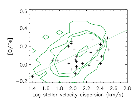
Figure 1: The [$<O/Fe>$]_core-$\sigma$ relation predicted for our model ellipticals and bulges shown as crosses in the figure. Data from Thomas et al. (2007) are shown as contours. A liner regression to Thomas et al. (2007) is shown by a thin solid line. Note that in this plot we rescaled our [$<O/Fe>$] values in order to be consistent with the solar abundances used by Thomas et al. (2007). Spiral bulges obey to the same relation (Thomas & Davies, 2006).

4.1 Elliptical galaxies

In brief, we first recall from Paper I how the formation of a galaxy proceeds in our model. We take the case La as an example. At times earlier than 300 Myr the gas is still accumulating in the central regions where the density increases by several orders of magnitude, with a uniform speed across the galaxy. The temperature drops due to cooling, and the SF can proceed at a very high rate ($\sim 10^{2-3}\rm M_{\odot}yr^{-1}$), at variance with the outermost regions, that complete their build-up in the first 100 Myr. This implies that a metal rich medium, dominated by SNIa ejecta, pollutes the gas supply for the SF in the inner regions. After 400 Myr, the gas speed becomes positive (i.e. out-flowing gas) at large radii, and at 500 Myr almost the entire galaxy experiences a galactic wind. At roughly 1.2 Gyr, the amount of gas left inside the galaxy is below 2% of the stellar mass. This gas is very hot (around 1 keV) and still flowing outside.

The galactic wind occurs first in the outer regions and then in the more inner zones of the galaxy because the work to extract the gas from the outskirts is less than the work to extract the gas from the center of the galaxy. The age differences between internal and external zones, however, are less than 1 Gyr and this ensures that our models are globally $\alpha$-enhanced. In this way our models are consistent with the observed age gradients (references in Sec. 2) and with the [$\alpha$/Fe]-mass relation. The picture sketched above applies to the lower mass models presented here. The fact that in our galaxy formation scenario the metallicity gradients arise because of the different times of occurrence of galactic winds in different galactic regions implies that the stellar metallicity is a function of the local escape velocity $v_{esc}$ for all the galaxies. In fact, in the regions where $v_{esc}$ is low (i.e. where the local potential is weaker), the galactic wind develops earlier and the gas is less processed than in the regions where $v_{esc}$ is higher (see Martinelli et al. 1998). Such a relation as been originally suggested by several authors (e.g. Davies et al., 1993, Peletier et al., 1990) and now confirmed by Scott et al. (2009). Here we can also show that the local index-$v_{esc}$ trend matches the global scaling (Scott et al., 2009). In particular, we make use of the definition $v_{esc}=\sqrt{(-2\Phi)}$, where $\Phi$ is the potential due to stars and DM, in agreement with the definition used by the observers. Some important caveats apply to this comparison. In observations, $v_{esc}$ depends on the modelling of the potential. Moreover, our models are spherically symmetric, whereas observed galaxies are not. In Fig. 2 we show that metallicity (given by the index $Mg_{b}$) versus $v_{esc}$ gradient slope for our models. The central $Mg_{b}$ value for each model galaxy is given by an asterisk, whereas the value at 1 $R_{eff}$ by a cross. Each couple of points connected by a line represents a galaxy: this is the local relation. The dashed line is the observational global (i.e. the fit to the central values of $Mg_{b}$ and $v_{esc}$ in observed galaxies) trend reported by Scott et al. (2009) along with the 3$\sigma$ dispersion (dotted lines). We show that the models presented in this paper reproduce the observed trend within the observed scatter. The fact that the each galactic region follows the global trend strongly suggests the idea that a uniform process - like the monolithic collapse - is behind the formation of the gradients.

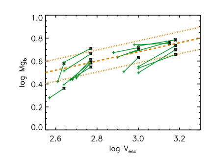
Figure 2: Metallicity versus $v_{esc}$ gradient slope for our models. The central $Mg_{b}$ value for each model galaxy is given by an asterisk, whereas the value at 1 $R_{eff}$ by a cross. Each couple of points connected by a line represents a galaxy (the local relation). The dashed line is the global relation (Scott et al., 2009) along with the 3$\sigma$ dispersion (dotted lines).

Table 2: Model results

Model	$M_{*}$	$R_{eff,*}$	[$<O/Fe>_{*,core}$]	$\Delta_{O/Fe}$	$\Delta_{Z/H}$
	($10^{10}M_{\odot}$)	(kpc)
Massive ellipticals (Paper I)
Ma1	6.0	12	0.29	0.02	-0.19
Ma2	25.	7.7	0.22	-0.21	-0.52
Ma3	25.	8.3	0.35	-0.17	-0.03
Mb1	6.0	17	0.14	0.09	-0.20
Mb2	3.0	8.7	0.33	0.	-0.18
Mb3	21	8.8	0.17	-0.08	-0.34
Mb4	26	5.4	0.42	-0.08	-0.20
La	26	29	0.14	0.19	-0.50
Lb	29	21	0.12	0.32	-0.30
Low mass ellipticals
E1a	0.74	1.7	0.08	-0.04	-0.26
E1b	0.74	1.7	0.36	-0.13	-0.21
E1c	0.74	1.7	0.28	-0.11	-0.21
E2a	1.5	0.9	0.19	-0.03	-0.29
E2b	1.8	0.6	0.14	+0.01	-0.29
E2c	1.4	0.89	0.26	-0.04	-0.30
E2d	0.27	2.3	0.17	+0.01	-0.29
E3a	0.88	1.6	0.18	-0.005	-0.27
E3b	0.65	1.1	0.11	+0.07	-0.28
E3c	0.93	1.6	0.09	-0.01	-0.32
E3d	0.6	1.1	0.03	+0.06	-0.25
E4a	1	1.7	0.16	-0.21	-0.33
E4b	0.35	0.6	0.22	-0.04	-0.36
E4c	0.05	0.5	0.17	-0.01	-0.22
E5	1	1.7	0.16	-0.20	-0.38
E6	1	1.7	0.11	-0.16	-0.34
Bulges
bulge1	0.06	2	0.	0.09	-0.36
bulge2	1.8	1	0.40	-0.07	-0.22
bulge3	2.3	0.8	0.3	0.07	-0.36
bulge4	3.7	0.7	0.29	0.00	-0.37
bulge5	1.0	0.4	0.28	0.00	-0.30

Models called E are low-mass ellipticals, whereas models called bulge are spiral bulges. Values predicted after the SF has finished.

Figure 3: Metallicity profiles predicted by our model ellipticals.

4.2 Galaxy bulges

Remarkably, all the results discussed in the previous sections apply to smaller objects (but embedded in much more massive haloes) such as the galaxy bulges, although the gradient slopes are slightly smaller (see entries in Table LABEL:table2). The main difference is that, due to their host galaxy potential well, strong and long lasting winds do not develop. We also find that the bulge formation is fast in agreement with the original suggestion by Matteucci & Brocato (1990), Elmegreen (1999) and the more recent work by Ballero et al. (2007).

We take advantage of the classical bulges as a further tool to calibrate our models. Indeed, in Paper II (where we refer the reader for further details) we compared our model predictions to the properties of the resolved stellar population observed in the Milky Way bulge by using the model bulge3 and found a remarkable agreement. This model has a stellar mass of $\sim 2\times 10^{10}M_{\odot}$ and a radius of $\sim 1$kpc in order to match the observed properties of our own Galaxy bulge (e.g. Minniti & Zoccali, 2008). The same model reproduces the chemical constraints coming from the Bulge integrated light, in that it predicts the following values for the indices H_β=1.61, $Mg_{2}$=0.29 and $<Fe>$=2.46 in good agreement with the observed values of H_β=1.5$\pm$0.6, $Mg_{2}$=0.23$\pm$0.04 and $<Fe>$=2.15$\pm$0.4 (Puzia et al., 2002). This is an important point that must be stressed: the abundance (and abundance gradients) that may be inferred from the analysis of Lick indices are average values. With resolved stellar populations (Paper II) is possible to show that the models presented here not only explains the average values, namely the mean properties of a Composite Stellar Population (CSP), but also their evolution in the [$O/Fe$]-[$Fe/H$] plane, namely the composition of each SSPs that make a CSP. Our fiducial model assumes Salpeter (1955) IMF, which successfully reproduces the properties of massive spheroids. In Paper II we show that the stellar metallicity distribution predicted by such a model reproduces the observed K-giant metallicity distributions for the Milky-Way bulge. We refer to Paper II (c.f. Fig. 2) for the test of other possible IMFs, motivated by either observations or theoretical efforts, which seems more appropriate for bulges.

The reader should note that we present several other models for bulges which do not necessarily have properties - such as stellar mass or radius - similar to those of the Milky Way bulge.

5 The predicted gradients

In this section we turn our attention on the main topic of this work and investigate the possible dependence of the gradient slope - and its scatter - from either the stellar mass or some mass tracers. We first focus on the actual prediction from the modeller’s point of view, namely gradients in abundance and abundance ratios versus mass and central [$<$O/Fe$>$], whereas we refer to Sec. 5.2 for our model predictions transformed into observational line-strength indices.

The metallicity profiles predicted by our model ellipticals over the 0.1-1$R_{eff}$ range are shown in Fig. 3. In the vast majority of the cases we predict a linear decrease of the metallicity with log (r) and thus justifies the adopted definition for $\Delta_{Z/H}$. We refer the reader to Paper I (Fig. 8) comparison between the observed and predicted [O/Fe] profiles for some relevant cases.

For elliptical galaxies we make use of Mehlert et al.’s (2003) and Annibali et al.’s (2007) datasets, whose samples are larger than Ogando et al.’s one, although the former do not find such a strong correlation between gradient slope and mass as the latter (other works with less galaxies are not taken into account in order not to have a poor statistics). For bulges we adopt the data from Jablonka et al. (2007), who explore a range in velocity dispersions similar to the above- mentioned articles. Unfortunately, we cannot use a homogeneous set of observables to constrain both the theoretical and the observational predictions for several reasons. In the first place, in several articles the authors do not extract the [$<$O/Fe$>$] abundance ratio gradient from their line-strength indices (e.g. Ogando et al. 2005, Kobayashi & Arimoto 1999, and Sanchez-Blazquez et al. 2006). Secondly, in all cases the stellar mass is not observed, whereas only the stellar velocity dispersion is given. Finally, several authors rely on a different sub-set of the Lick line-strength indices to infer the metallicity.

5.1 Theoretical relations with mass and mass tracers

With the above mentioned caveats in mind, in Fig. 4 we present our predictions regarding the theoretical relation between abundance gradients and mass tracers (namely the stellar velocity dispersion and the central [$<O/Fe>$]). The remainder of this section is devoted to fully describe Fig. 4.

5.1.1 Gradients in metallicity

Let us first focus on the upper row of Fig. 4: the total metallicity gradient. In the left panel we show the [$<Z/H>$] gradient slope in the stellar component predicted by our model for ellipticals (hollow circles) and bulges (full dots) as a function of the stellar mass when all galaxies are considered. This is the actual prediction of our models. Formal linear regression fits to the entire sample of model galaxies (solid line), to the galaxies with steepest gradients (dotted line ) and to dwarf ellipticals (dashed line) are shown. We predict a very mild trend in mass. In the high mass region, our model predictions span a range in the gradient slopes similar to the observed values. Neither our models, nor the three observational samples (taken togheter) show any sign of (anti-)correlation as suggested by the single authors. We therefore conclude that, in this mass range, is more appropriate to speak of an increase in the scatter of the gradient slope at a fixed mass. If we take only the four less massive objects we find a quite steep relation between metallicity gradient and galaxy mass, parallel to the locus of the galaxies with the steepest gradients (we call it the maximum steepness boundary line) similar to the predictions of the earlier monolithic collapse models. This finding seem to be in qualitative agreement with the observational results by Spolaor et al. (2009). As for the points near the maximum steepness boundary, they always refer to the models with the highest SF efficiency at that given mass. We note another trend, symmetric to maximum steepness boundary with respect to the solid line (trend of the entire sample), in the sense that at the highest masses we have also the flattest gradients. This seems to go in the direction of Ogando et al. (2005), Spolaor et al. (2009) and Jablonka et al. (2007) results. In particular, the scatter is minimum at masses below $\sim 10^{10}M_{\odot}$. These galaxies tend to have neither shallow metallicity gradients nor very steep ones.

In order to explain such findings, we first note that the formal linear regression to our model predictions gives $\Delta_{Z/H}\sim-0.04\,log\,\sigma$, namely a value much smaller (in absolute value) than the slope of the mass-metallicity relation $[Z/H]_{core}\sim 0.57\,log\,\sigma$. Therefore the relation between gradient slope and galactic mass cannot be explained by the Carlberg (1984)’s argument (c.f. Introduction, see also Jablonka et al. 2007). In other words, the steepening of the gradient with mass is not due to the sole increasing metallicity of the galactic core, whereas the outermost regions of galaxies differing in mass keep the same value for [$<Z/H>$]_eff. Indeed it has been shown observationally that the metallicity of the entire galaxy should obey to the mass-metallicity relation (e.g. Graves et al. 2007). Such a relation is satisfied by our models, for which we predict $[Z/H]_{eff}\sim 0.53\,log\,\sigma$. Hence $\Delta_{Z/H}\sim[Z/H]_{eff}(\sigma)-[Z/H]_{core}(\sigma)\sim 0.53\,log\,\sigma-0.57\,log\,\sigma=-0.04\,log\,\sigma$ . The reason for this increase in the global galaxy metallicity with mass is due to the fact that the entire galaxies, not only their central cores, should form more efficiently as their mass increases in order to comply with the downsizing trend, namely the need to have [$<\alpha$/Fe$>$] ratios greater than zero and positively correlated to the mass. This request renders the average gradient slope predicted by the revised monolithic models flatter than the earlier monolithic collapse models a la Larson. However, galaxies with steep gradients still exists (e.g. models La and Lb) and lie on the maximum steepness boundary. On average, galaxies with mass $\sim 10^{10}M_{\odot}$ feature gradient slopes quite close to the maximum steepness boundary, therefore the scatter is small. At larger masses, the average gradient is nearly one half of the maximum steepness boundary value at that mass, hence allowing for more intermediate possibilities.

It is interesting to understand what are the major causes for such a range although we have unevenly sampled the parameter space and despite the not very high number of simulated galaxies. We suggest that differences in the initial conditions of the protogalactic cloud(s) can reproduce the observed scatter. Here we discuss their relative role.

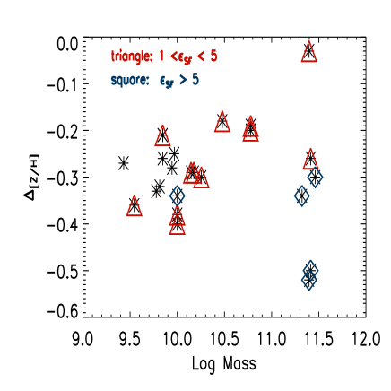
Figure 5: Predicted [$<Z/H>$] gradient slope as a function of the mass in the case of ellipticals only (asterisks). Models are further coded by their $\epsilon_{SF}$

• Especially at larger masses, the higher the star formation parameter $\epsilon_{SF}$, the steeper the gradient (see Fig. 5). As an example compare the model Ma2 with Ma3 (or models E6 and E2c). Their initial conditions are the same but for $\epsilon_{SF}$. The metallicity gradient predicted for the former model (which has a higher star formation parameter) is much steeper than the latter case. At the first order, the metal production scales with the SF rate. Therefore, the metallicity increases faster when $\epsilon_{SF}$ is increased and all the other parameters are held fixed. However, the SF depends also on the cooling, that increases at higher metallicity, and the local gas density. Another important factor in regulating the SF is the interplay between stellar feedback and local potential. Taking togheter all these factors, in the case in which the gas is already in place, the net product is that augmenting $\epsilon_{SF}$ leads to a faster increase (relatively speaking) in the metallicity of the central regions, where the potential is very deep and the gas is denser than in the outskirts, where an higher SF rate also implies that the conditions for the wind set in earlier.

• The role of the chosen profile is slightly less evident. On average, the flat profile leads to slightly steeper gradients. For instance, compare model Mb4 with Ma1 that share the same initial condition but the profile. Similarly, compare model E1b to E1a. This happens because, while in the IS models most of the (pristine) gas is already in place, in the flat models the majority of the gas supply to build the inner regions has go through the outskirts when being accreted. Hence, the sinking gas is polluted by metals, leading to a faster metal enrichment of the inner regions. However, this effect is weaker than that caused by $\epsilon_{SF}$. For instance compare model Ma2 with Mb4.

• As for the temperature, starting from a higher value implies a longer time for cooling the gas and feeding the star formation process. In a sense, the effect is similar to the difference between the flat case versus the IS case. For instance, on the basis of the previous point we would expect model Ma1 to exhibit a (slightly) shallower gradient than the one of model Ma3. Instead it is steeper. However, a higher initial temperature is not enough to counterbalance the effect of a large change in $\epsilon_{SF}$ (see model Ma1 versus model Ma2).

• For flat models, the initial gas density seems to be relatively unimportant (e.g. compare models E2c and E4c) in the determining the slope of the metallicity gradient.

In conclusion, we do not find a parameter that fully governs the creation of the gradient, even if $\epsilon_{SF}$ seems to be quite important. Different - but reasonable - combination of the input parameters lead to model properties that obey both the overall properties observed in elliptical galaxies and exhibit average metallicity gradient of -0.3 dex per decade in radius. Changes in the initial conditions within the same broad formation scenario create the scatter in the predicted gradients at a single mass. These changes, therefore, should not be ascribed to different pictures for the formation of the galaxies. They rather mimic cases in which the accretion from the proto-galactic clouds may be faster (e.g. the IS cases) or proceed through cold accretion through filaments (Dekel & Birnboim, 2006, the flat case). They also show the different behaviour of models where the star formation is favored (higher $\epsilon_{SF}$, e.g. for the formation of the most massive galaxies) or disfavored (models with high initial temperature: the gas is accreted in pre-existing haloes and has to cool before forming stars).

In the middle and right panels in the upper row of Fig.  4 we compare our model predictions to metallicity gradients inferred from observations (Mehlert et al 2003, Annibali et al. 2007, Jablonka et al. 2007). Obviously the above discussion on the cause of the (scatter in the) metallicity gradient applies also to the other mass tracers ($\sigma$ and the central [$<O/Fe>$]). As explained above, however, here we can compare our predictions with the values measured by the observers. We can thus show that the predicted range as well as the average gradient slope (-0.3 dex per decade in radius) are in agreement with observations. We note how different observational groups infer slightly different mean $\Delta_{Z/H}$ (e.g. compare the samples in Fig. 4). For instance in the literature average values either as low as $-0.22\pm 0.1$ or as high as $-0.34\pm 0.08$ (Brough et al., 2007) can be found. Still consistent with each other, though. This might be due to a different combination of line-strength indices used to infer the variation in metallicity (see the analysis in Sanchez-Blazquez et al. 2006). Also differences in the SSP library used to transform indices into abundances can create the offset. Moreover, small number statistics can still bias the results as well as the fact that, even in the same sample, metallicity gradients are not measured out to the same radius. Some authors claim the difference is caused by the environment, with field ellipticals featuring shallower gradients on average with respect to galaxies living in higher density regions (Sanchez-Blazquez et al. 2006). Such a suggestion might explain the offset between the Mehlert et al. (2003) Coma cluster ellipticals and the Annibali et al. (2007) spheroids.

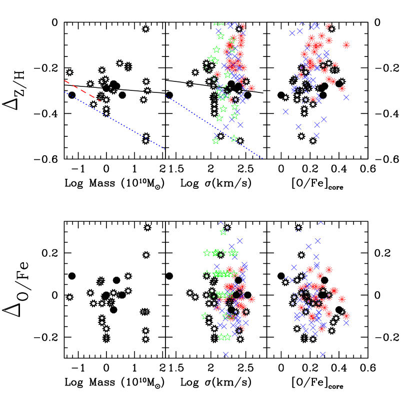
Figure 4: Theoretical predictions versus abundance gradients inferred from observations. Upper panels: Predicted [$<Z/H>$] gradient slope in the stellar component of our model ellipticals (hollow circles) and bulges (full dots) as a function of the stellar mass and other mass tracers (namely the stellar velocity dispersion and the central [$<O/Fe>$]). Formal linear regression fits to the entire sample (solid line), to the galaxies with steepest gradients (dotted line, the maximum steepness boundary) and to dwarf ellipticals (dashed line) are shown. Data from Mehlert et al. (2003, asterisks, red), Annibali et al. (2007, crosses, blue) and Jablonka et al. (2007, stars, green) are shown. Lower panels: As above, but for the [$<O/Fe>$] gradient.

5.1.2 Gradients in abundance ratios

We now move to the analysis of the bottom row of Fig. 4. No clear relation with mass is found for the [$<$O/Fe$>$] radial gradients. Indeed, as expected from Paper I and II, most of our models predict a nearly flat [$<O/Fe>$] gradient, with some showing either positive or negative slopes.

In particular, we suggest the gradient in the [$<\alpha$/Fe$>$] ratio to be related to the interplay between the velocity of the radial flows moving from the outer to the inner galactic regions, and the intensity and duration of the SF formation process at any radius. Clearly a larger or smaller parameter of star formation can have a strong influence on this process. This result implies that we do not need the merger events in order to have a shallow [$<\alpha/Fe>$] gradient.

In general, we find that in our models with $\Delta_{O/Fe}\leq 0$ the role of both the gas flowing inward and the star formation timescale increasing at large radii is non negligible. The role of the initial temperature can be important. If the galaxy formation process starts from hot gas (i.e. $10^{6-7}$ K), we predict $\Delta_{O/Fe}\geq 0$ in the majority of the cases. They are thus similar to the quasi-monolithic chemical evolution models of Pipino & Matteucci (2004, PM04) with not interacting shells in which the infall timescale increases at shorter radii, whereas the star formation efficiency is constant. On the other hand, models starting with cold (i.e. $10^{4-5}$ K) gas seem to prefer a negative $\Delta_{O/Fe}$.

The sole SF efficiency seems to affect the predicted absolute value of the gradient slope; in fact all the models most effective in forming stars exhibit the steepest slopes at the same time. Basically, an increase in the SF efficiency enhances the differences between the inner core and the outskirts set by the other initial conditions. For instance, if the gas is already in place, a high efficiency in forming stars boosts the outside-in process. In such a case, the star formation process, which also locks the metals into the stars, is fast enough in the central regions to avoid the contamination of the metals flowing from larger radii. In practice we end up in the extreme case in which the gas flows can be neglected and $\Delta_{O/Fe}\sim 0.2$ as in the standard chemical evolution models (Pipino et al. 2006).

5.1.3 Correlations between gradients in metallicity and gradients in abundance ratios

The final part of the theoretical analysis involves the study of possible correlations between gradients in metallicity and gradients in abundance ratios. As a confirmation of what said in Sec. 5.1.2, galaxies showing the steepest positive [$<$O/Fe$>$] gradient slopes, have also quite a strong radial decrease in the [$<$Fe/H$>$] ratio (Fig. 6). These galaxies are also the most massive ones. A correlation in this sense seems to be confirmed by the Annibali et al. (2007) data, whereas Mehlert et al.’s (2003) galaxies exhibit values for $\Delta_{O/Fe}$ constant with $\Delta_{Fe/H}$. A quantitative confirmation needs a sample statistically richer. Perhaps more interestingly, neither the observations nor the models cover the region with $\Delta_{O/Fe}<0$ and $\Delta_{Fe/H}<-0.4$: galaxies with the steepest metallicity gradients undergo a strong outside-in formation process. In galaxies with $\Delta_{O/Fe}<0$ - namely, models that likely have a local star formation efficiency decreasing with galactocentric radius - the stellar feedback is more effective in contrasting the metal-enhanced flows; therefore, the final $\Delta_{Fe/H}$ is smaller (in absolute value), hence closer to the expectations from models which do not take into account gas flows within the galaxy. At the same time we predict a paucity of galaxies in the region $\Delta_{O/Fe}>0$ and $\Delta_{Fe/H}>-0.2$. More observations are needed to confirm this suggestion. A lack of galaxies can also be noticed in the upper left corners on the left panels in Fig. 4.

.

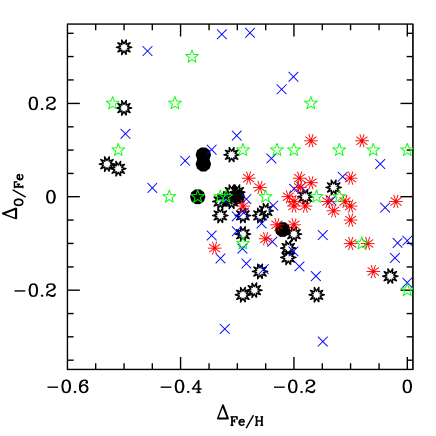
Figure 6: Predicted [$<O/Fe>$] gradient slope as a function of the [$<Fe/H>$] one. Symbols as in Fig. 4.

5.2 Gradients in line-strength indices

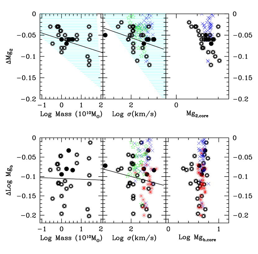
Figure 7: Comparison between model predictions and data in the observer’s plane. Upper panels: Predicted $Mg_{2}$ gradient slope as a function of the stellar mass and mass tracers. The hatched area represents the portion of the plane $\Delta Mg_{2}$-mass (-$\sigma$) allowed by the data from Ogando et al. (2005). Symbols and data as in Fig. 4. Lower panels: As in the upper panel, but for the $Mg_{b}$ index.

Before discussing the implication of our results, it is useful to re-cast the results of Fig. 4 in terms of their observational counterparts in order to enable a ready comparison between our model predictions and future observational samples. This is done in Fig. 7.

We transform the predicted metallicity and abundance ratios into line-strength indices by means of Thomas et al. (2003) SSPs. In practice, we interpolate the Thomas et al.’s theoretical library in order to get a value for the indices Mgb and Mg₂ for each combination of age, metallicity and $\alpha$-enhancement at any given radius. For simplicity we assume a fixed 12 Gyr old population and that the age radial gradient are always negligible, since our models always predict age differences lower than 0.5-1 Gyr.

In the upper panels of Fig. 7 we present the results for the index $Mg_{2}$ as a function of the stellar mass and stellar velocity dispersion. Instead of the central [$<O/Fe>$], here we use the central value for the index, since it correlates with mass. The solid lines are formal linear regression fits to the models. The hatched area represents the portion of the plane $\Delta Mg_{2}$-mass (-$\sigma$) covered by the data from Ogando et al. (2005). First, we note that the trends in the theoretical metallicity gradients with mass is confirmed when translated into observables. In particular we confirm the presence of a boundary that corresponds very well findings by Ogando et al. (2005), whereas the mean predicted slope ($d\rm Mg_{2}/log(R_{eff,*}/R_{core,*})\sim-0.06$ mag per decade in radius) is shallower than this limit at any mass. We recall that a one-to-one correspondence between index gradient and metallicity gradient cannot be done, since the transformation depends also on [$<$O/Fe$>$] and age. This is the main reason why we based our interpretation on Fig. 4 rather than on Fig. 7.

As expected, the region of the planes index-mass tracer covered by our model predictions overlaps with those of the actual data from the observational samples (Mehlert et al 2003 - red triangles; Annibali et al. 2007 - blue triangles; Jablonka et al. 2007, yellow; see also Sanchez- Blazquez et al., 2006, not shown here) that we employed in the previous sections.

No trend appears when we show the predictions regarding the $Mg_{b}$ index (Fig. 7, lower panels). We show this discrepancy as a warning: trends can be strongly index-dependent (see also Sanchez-Blazquez et al. 2006). The same relation between a theoretical metallicity profile and the galactic mass can lead to a different gradient-mass behaviour in the observer plane, depending on the chosen index. According to Jablonka et al. (2007), such a dichotomy between these two indices should be related to Mg is due to the C abundance that plays a role in the index strength. Also the role of the age gradients cannot be neglected.

6 Discussion

In this paper we showed that difference in the degrees of dissipation, in the times at which the galactic wind occurs and star formation histories alone can explain the observed scatter within a quasi-monolithic assembly. At variance with other authors (Kobayashi 2004) we do not need differing channels (i.e. “truly monolithic” galaxies, “truly hierarchical” galaxy and a mixture of these two) to cover the range of observed gradient slopes. In a companion paper (Di Matteo et al., 2009) we show, instead, that equal mass dry-mergers between ellipticals systematically lower (by a factor of $\sim$ 2) the slope of the pre-existing gradient. Therefore we argue that if one wants to explain the scatter observed by Ogando et al. (2005), Spolaor et al. (2009) and Jablonka et al. (2007) in the gradient slopes at high masses with the effects of dry-mergers one can accommodate only a few of such episodes, otherwise we would observe only galaxies with flat gradients. This is true unless there is a channel that continuously provides galaxies with the steepest gradients (i.e. -0.5 dex per decade in radius) that then can undergo mergers. These ellipticals clearly cannot come from mergers, otherwise we would need progenitors with slopes even steeper than the early monolithic collapse models of Larson and Carlberg (i.e. -0.5 to -1 dex per decade in radius, see Introduction). Hence the majority of ellipticals have presumably formed in a monolithic fashion even if we allow some dry-mergers to occur. Therefore we refer to dry mergers as possible (but not necessary) episodes in the galaxy life which may change the gradient rather than to a well-defined channel for galaxy formation which co-exists with the monolithic channel as in Kobayashi (2004). Similar constraints on the number of dry mergers can be obtained by the [$<\alpha$/Fe$>$]-mass relation (Pipino & Matteucci, 2008).

As far as the wet mergers are concerned, it is argued that they may steepen the gradients if star formation takes place in the metal rich gas funneled towards the galactic core (Hopkins et al., 2008). Such a mechanism, however, creates strong features in the age profiles - at variance with observations - that may disappear only after several Gyr if the galaxy evolves in isolation since then, at the expenses of a flattening of the metallicity gradient. Unfortunately, Hopkins et al’s simulation are not done in a cosmological context and start from very simplistic assumptions (zero metallicity disks), therefore it is not clear what happens when the simulated galaxy undergoes several mergers as predicted in the hierarchical formation scenario. According to Kobayashi (2004), the steepening of gradients by the secondary star formation (i.e., wet merger) seems to occur only rarely. Moreover, we expect these gradients to be erased by subsequent dry mergers. Furthermore, it has been shown (Pipino et al., 2009a) that the hierarchical formation is still incompatible with the observed [$\alpha$/Fe]-mass relation in ellipticals. On the other hand, a clear forecast of our model is non-evolving metallicity gradients in time, apart from the effects of the passive luminosity evolution on the galaxy spectrum.

Another prediction of our models is the correlation between [$<$O/Fe$>$] and [$<$Fe/H$>$] gradients, in the sense that we expect galaxies with the steepest [$<$Fe/H$>$] gradients to have a very low [$<$O/Fe$>$] abundance ratio in the core; therefore such galaxies must exhibit a very steep and positive [$<$O/Fe$>$] gradient. This does not translate into a clear correlation between the [$<$O/Fe $>$] gradient and the mass because of the large scatter which erase any clear signal.

Before concluding, we wish to discuss some assumptions, limitations and implications of the present study.

The initial conditions where chosen in order to reproduce the typical present-day colours, SF rates (as observed in high redshift progenitors) and central [$<$O/Fe$>$], [$<$Z/H$>$] values for elliptical galaxies. Preliminary exploration of the parameter space led us to restrict our analysis to a range 0.1-10 in the star formation parameter $\epsilon_{SF}$, 10^4-7K in the initial temperature, 10% SN efficiency. The majority of the resulting models show metallicity profiles linearly decreasing with log radius, stellar mass to light ratios and radii in agreement with observations.

As a first approximation, our bulge models do not take into account the presence of a disk. This is justified by the following two reasons: the disk forms on a much longer timescale (e.g. Zoccali et al., 2006 Matteucci & Brocato, 1990, Ballero et al.,2007) and current observational samples have been derived by accurately selecting edge-on galaxies where the contamination from the discs should be minimal. However we stress that our results for the bulges might be less constrained and robust that those concerning elliptical galaxies and further investigation is needed.

The number of modelled galaxies is small, and hence can suffer from the same small number statistics that bias the observations. We therefore avoided any specific prediction on the mean trend of both the metallicity and the [$<$O/Fe$>$] gradient with mass. The formal linear regressions shown in the figures are for the mere purpose of guiding the eye and the exact positioning of the maximum steepness boundary might depend on the portion of the parameter space explored. We stress that the main purpose of the paper is to show that even in the monolithic formation collapse a range in the predicted gradients consistent with observations must be expected and that a typical metallicity decrease of 0.2 dex out to 1 $R_{eff}$ can be easily reproduced by recent monolithic collapse models. This result is robust, because even if the models presented here do not cover the entire parameter space, the range in predicted gradients cannot be decreased by adding other models. The statistical scatter may change; however observational samples likely suffer from the same small number statistics problem: this is why we avoided any detailed statistical analysis in the present study. The presence of elliptical galaxies with flatter gradients than the original models by Carlberg (1984) should not be used as an evidence for mergers.

The metallicity profiles of some of the galaxies with the steepest gradients slightly depart from linearity (c.f. Fig. 3). We would predict a shallower gradient than the one reported in Table 2 if we limited our analysis to the inner  1/3 $R_{eff}$; vice-versa the predicted gradient would be steeper if we were to consider only the region  1/3 - 1$R_{eff}$. Therefore, we caution the reader that the conclusions about the steepest gradients in our model galaxies and their relation with the monolithic boundary might depend on the chosen radius. A detailed comparison between model profiles and single well studied galaxies over a large mass range will allow us to study the metallicity gradients in their finer details and better constrain the models presented here.

Moreover, while most of our models obey to the mass-size relation for ellipticals (e.g. Shankar et al., 2010), some galaxies with similar mass (e.g. compare models Ma2 and La) have quite different radii. The former model has a radius consistent with those for normal ellipticals of that mass (e.g. Shankar et al. 2010), the latter is more typical of an early type Brightest Cluster Galaxy (BCG, e.g. Graham et al., 1996). We chose not to make any distinction between BCGs and normal ellipticals in our models since gradients measured in BCGs have traditionally been included in the sample as the ones that we use and because there is no difference as far as the chemical properties are concerned (e.g. von der Linden et al., 2007, Brough et al., 2007). However the reader should keep in mind that a structural difference between BCGs and normal ellipticals seems to exist, and BCGs seem to harbor steep gradients (e.g. Brough et al., 2007). Therefore, in light of the special role of BCGs (e.g. Pipino et al., 2009b, von der Linden et al., 2007, and references therein), further and dedicated observations and modelling are required to ascertain if there is any systematic difference in the metallicity gradients with respect to more ordinary ellipticals and what is the cause.

Also, we remind that the majority of the observational works use Mg as a proxy for the $\alpha$ elements, as can be easily observed in absorption in the optical bands giving rise to the well known $Mg_{2}$ and $Mg_{b}$ Lick indices. However, the state-of-the-art SSPs libraries (Thomas et al. 2003, Lee & Worthey, 2009) are computed as functions of the total $\alpha$-enhancement and of the total metallicity. This is true also for the stellar tracks, where the O abundance dominates the opacity, and hence the stellar evolution. The latest observational results (Mehlert et al. 2003, Annibali et al. 2006 and Sanchez-Blazquez et al. 2007) that we contrasted to our predictions in this study, have been translated into theoretical ones by means of these SSPs; therefore the above authors provide us with radial gradients in [$\alpha$/Fe], instead of [Mg/Fe]. This is why in this paper we focus on the theoretical evolution of the $\alpha$ elements by using O that is by far the most important.

Here we briefly recall that both O and Mg come from the hydrostatic burnings in massive stars, therefore they are produced in lock-step. It has been suggested recently (e.g. McWilliam et al., 2007) that this might not be true at solar (and above solar) metallicities. While this is an important effect in detailed chemical evolution studies it has no importance when the luminosity weighted properties of a composite stellar population are concerned. This happens because luminosity averages weigh more the stellar populations at lower metallicities (lower M/L), where the differences between O and Mg production are negligible (if any). Finally, even if the abundance of O and Mg are offset by some fixed quantity (i.e. [O/H]=[Mg/H]+const), the predicted gradient would be the same.

7 Conclusions

In this paper we study the formation and evolution of ellipticals and bulges by means of a hydrodynamical model (c.f. Paper I and II, respectively) in order to understand the origin of the observed scatter in the abundance gradients of early type galaxies. Here we summarise our main results.

• We find $\Delta_{Z/H}$ in the range -0.5 – -0.2 dex per decade in radius with a mean value of -0.3 dex per decade in radius, in agreement with the observations (e.g. Kobayashi & Arimoto, 1999).

• In agreement with Ogando et al. (2005) and Jablonka et al. (2007), we find that that the scatter in the gradient slopes increases as a function of mass. We reproduce such a scatter in the observations by means of variation in the initial conditions in galaxy models.

• Model galaxies which behave as the earlier monolithic collapse models by Larson (1974) and Carlberg (1984) define a maximum steepness boundary in the metallicity (and index) gradient slope-mass plane. These galaxies are preferentially those with the highest star formation efficiency at that given mass.

• No galaxies with gradients steeper (i.e. more negative) than the value given by the our predicted theoretical boundary are observed (Ogando et al., 2005, and Spolaor et al., 2009, for ellipticals and Jablonka et al., 2007, for bulges).

• No correlation between $\Delta_{O/Fe}$ and other galactic properties are found, in agreement observations for ellipticals (Mehlert et al., 2003, Annibali et al., 2007) and bulges (Jablonka et al., 2007).

• The abundance gradients in the abundances, once transformed into line-strength indices, lead to $dMg_{2}/log(R_{core,*}/R_{eff,*})\sim-0.06$ mag and $dLogMg_{b}/log(R_{core,*}/R_{eff,*})\sim-0.1$ per decade in radius, again in agreement with the typical mean values measured for ellipticals and bulges.

• We note that the behaviour of the gradient slope as a function of the galactic mass strongly depends on the particular line-strength index used. In fact, the predicted $Mg_{2}$ index gradient seems to correlate with mass, whereas the $Mg_{b}$ index gradient does not.

• In Paper I we demonstrated that the differential occurrence of galactic winds (outside-in formation) alone can explain the existence of the metallicity gradients discussed in this paper. Here we add that this mechanism predicts a tight correlation between line-strength index and escape velocity gradients which has been confirmed by recent data (see Scott et al., 2009).

Larger, homogeneous and statistically meaningful observational sample of gradients in elliptical galaxies out to one effective radius can confirm such a prediction and validate the model.

References

- [] Annibali, F.; Bressan, A.; Rampazzo, R.; Zeilinger, W. W.; Danese, L., 2007, A&A, 463, 455
- [] Arimoto, N., Yoshii, Y. 1987, AA, 173, 23
- [] Asplund M., Grevesse N., Sauval A. J., 2005, ASPC, 336, 25 E.A., 2007, A&A, 497, 991
- [] Ballero, S., Matteucci, F., Origlia, L., Rich, R.M., 2007, A&A, 467, 123
- [] Bedogni, R. & D’Ercole, A., 1986, A&A, 157, 101
- [] Bekki, K., Shioya, Y. 1999, ApJ, 513, 108
- [] Brough, S.; Proctor, Robert; Forbes, Duncan A.; Couch, Warrick J.; Collins, C. A.; Burke, D. J.; Mann, R. G., 2007, MNRAS, 378, 1507
- [] Burstein, D., Bender, R., Faber, S.M., Nolthenius, R. 1997, AJ, 114, 1365
- [] Carlberg, R.G., 1984, ApJ, 286, 403
- [] Carollo, C.M., Danziger, I.J., Buson, L. 1993, MNRAS, 265, 553
- [] Chiosi, C., Carraro, G. 2002, MNRAS, 335, 335
- [] Ciotti, L., D’Ercole, A., Pellegrini, S., Renzini, A. 1991, ApJ, 376, 380
- [] Davies, R.L., Sadler, E.M., Peletier, R.F., 1993, MNRAS, 262, 650
- [] Dekel, Avishai; Birnboim, Yuval 2006, MNRAS, 368, 2
- [] Di Matteo, P., Pipino, A., Lehnert, M.D., Combes, F., Semelin, B., 2009, A&A, 499, 427
- [] Elmegreen, B.G. 1999, ApJ, 517, 103
- [] Forbes, D.A., Sanchez-Blazquez, P., Proctor, R., 2005, MNRAS, 361, 6
- [] Gonzalez, J.J., Gorgas, J. 1996, in ASP Conference Series, 86, Fresh Views of Elliptical Galaxies, eds. A. Buzzoni, A. Renzini, A. Serrano, 225
- [] Goudfrooij, P., Gorgas, J., Jablonka, P., 1999 Ap&SS, 269, 109
- [] Graham, A., Lauer, T.R., Colless, M. & Postman M., 1996, ApJ, 465, 534
- [] Graves, G.J., Faber, S.M., Schiavon, R.P., Yan, R. 2007, ApJ, 671, 243 Societa Astronomica Italiana, vol. 54, p. 311
- [] Iwamoto, K.; Brachwitz, F.; Nomoto, K.; Kishimoto, N.; Umeda, H.; Hix, W. R.; Thielemann, F.K. 1999, ApJS, 125, 439
- [] Jablonka, P., Gorgas, J. & Goudfroij, P. 2007, A&A, 474, 763
- [] Kawata, D. 2001, ApJ, 558, 598
- [] Kobayashi, C., 2004, MNRAS, 347, 740
- [] Kobayashi, C., Arimoto, N., 1999, ApJ, 527, 573
- [] Koleva, Mina; de Rijcke, Sven; Prugniel, Philippe; Zeilinger, Werner W.; Michielsen, Dolf 2009b, MNRAS, 396, 2133
- [] Koleva, M.; Prugniel, Ph.; De Rijcke, S.; Zeilinger, W. W.; Michielsen, D. 2009a, AN, 330, 960
- [] Kormendy, J., & Kennicutt R.C. 2004, ARA&A, 42, 603
- [] Larson, R.B. 1974, MNRAS, 166, 585
- [] Lee, Hyun-chul; Worthey, Guy; Dotter, Aaron, 2009, AJ, 138, 1442
- [] Martinelli, A., Matteucci, F., Colafrancesco, S., 1998, MNRAS, 298, 42
- [] Matteucci, F., & Brocato, E. 1990, ApJ, 365, 539 Galaxy, Kluwer Academic Publishers, Dordrecht 154, 279
- [] Matteucci, F.,Recchi, S., 2001, ApJ, 558, 351
- [] McCarthy, I.G.; Bower, R.G.; Balogh, M.L. 2007, MNRAS, 377, 1457
- [] Mehlert, D.; Thomas, D.; Saglia, R. P.; Bender, R.; Wegner, G. 2003, A&A, 407, 423
- [] Minniti, Dante; Zoccali, Manuela 2008, in “Formation and Evolution of Galaxy Bulges”, Proceedings of the International Astronomical Union, IAU Symposium, Volume 245, p. 323-332
- [] Nelan, J.E.; Smith, R.J.; Hudson, M.J.; Wegner, G.A.; Lucey, J.R.; Moore, S.A.W.; Quinney, S.J.; Suntzeff, N.B. 2005, ApJ, 632, 137
- [] O’Connel, R.W. 1976, ApJ, 206, 370
- [] Ogando, R.L.C., Maia, M.A.G., Chiappini, C., Pellegrini, P.S., Schiavon, R.P., da Costa, L.N., 2005 ApJ, 632, 61
- [] Padovani, P., & Matteucci, F. 1993, ApJ, 416, 26
- [] Peletier, R.F., Davies, R.L., Illingworth, G.D., Davis, L.E., Cawson, M. 1990, AJ, 100, 1091
- [] Pipino, A., D’Ercole, A., Matteucci, F, 2008a, A&A, 484, 679 (Paper I)
- [] Pipino, A., Devriendt, J., Thomas, D., Silk, J., Kaviraj, S., 2009a, A&A, 505, 1075
- [] Pipino, A.; Kaviraj, S.; Bildfell, C.; Babul, A.; Hoekstra, H.; Silk, J. 2009b, MNRAS, 395, 462
- [] Pipino A., Kawata D., Gibson B. K., Matteucci F., 2005, A &A, 434, 553
- [] Pipino, A., Matteucci, F. 2004, MNRAS, 347, 968 (PM04)
- [] Pipino, A., Matteucci, F. 2008, A&A, 486, 763
- [] Pipino, A.,Matteucci, F, D’Ercole, A., 2008b, IAUS, 245, 19 (Paper II)
- [] Pipino, A.; Matteucci, F.; Chiappini, C. 2006 ApJ, 638, 739
- [] Proctor, R.N., Sansom, A.E., & Reid, I.N. 2000, MNRAS, 311, 37
- [] Puzia, T. H.; Saglia, R. P.; Kissler-Patig, M.; Maraston, C.; Greggio, L.; Renzini, A.; Ortolani, S. 2002, A&A, 395, 45
- [] Rawle, T.D., Smith, R.J., Lucey, J.R., & Swinbank, A.M., 2008, MNRAS, 289, 1891
- [] Salpeter, E.E., 1955, ApJ, 121, 161
- [] Sanchez-Blazquez, P.; Forbes, D. A.; Strader, J.; Brodie, J.; Proctor, R. 2007, 377, 759
- [] Sanchez-Blazquez, P.; Gorgas, J.; Cardiel, N., 2006, A &A, 457, 82
- [] Sarajedini, Ata; Jablonka, Pascale 2005, AJ, 130, 1627
- [] Scott, N., et al. 2009, MNRAS, 398, 1835
- [] Serra, P. & Trager, S., 2007, MNRAS, 374, 769
- [] Shankar, Francesco; Marulli, Federico; Bernardi, Mariangela; Dai, Xinyu; Hyde, Joseph B.; Sheth, Ravi K. 2010, MNRAS, 403, 117
- [] Spolaor, M., Forbes, D.A., Proctor, R.N., Hau, G.K.T., Brough, S. 2008, MNRAS, 385, 675
- [] Spolaor, M., et al 2009 ApJ, 691, 138
- [] Silich, S.A., & Tenorio-Tagle, G., 1998, MNRAS, 299, 249.
- [] Sutherland, R.S., Dopita, M.A. 1993, ApJS, 88, 253
- [] Thomas, D., Davies, R., 2006, MNRAS, 366, 510
- [] Thomas, D., Maraston, C., Bender, R., 2003, MNRAS, 339, 897
- [] Thomas D., Maraston C., Bender R., Mendes de Oliveira C. 2005, ApJ, 621, 673
- [] von der Linden, Anja; Best, Philip N.; Kauffmann, Guinevere; White, Simon D. M. 2007, MNRAS, 379, 867
- [] Yoshii, Y., & Arimoto, N., 1987, AA, 188, 13
- [] White, S.D.M., Rees, M.J., 1978, MNRAS, 183, 341
- [] Worthey, G., Faber, S.M., Gonzalez, J.J. 1992, ApJ, 398, 69
- [] Zoccali, M., et al. 2006, A&A, 457, 1