Transfer of optical spectral weight in magnetically ordered superconductors

Abstract

We show that, in antiferromagnetic superconductors, the optical spectral weight transferred to low frequencies below the superconducting transition temperature originates from energies that can be much larger than twice the superconducting gap $\Delta$. This contrasts to non-magnetic superconductors, where the optical spectrum is suppressed only for frequencies below $2\Delta$. In particular, we demonstrate that the superfluid condensate of the magnetically ordered superconductor is not only due to states of the magnetically reconstructed Fermi surface, but is enhanced by transfer of spectral weight from the mid infrared peak generated by the spin density wave gap. We apply our results to the iron arsenide superconductors, addressing the decrease of the zero-temperature superfluid density in the doping regime where magnetism coexists with unconventional superconductivity.

I Introduction

Optical measurements reveal crucial spectral and electromagnetic properties of a superconductorMattis58 ; Ferrell58 ; Tinkham59 . For example, the London penetration depth $\lambda$ can be determined from the low frequency dependence of the imaginary part $\sigma^{\prime\prime}\left(\omega\right)$ of the optical conductivity $\sigma\left(\omega\right)$:

$$\ \sigma^{\prime\prime}\left(\omega\rightarrow 0\right)=\frac{c^{2}}{4\pi\lambda^{2}\omega},$$ (1)

where $c$ is the speed of light. In addition, the superconducting gap $\Delta$ can be obtained from the real part of the optical conductivity, $\sigma^{\prime}\left(\omega\right)$, since spectral weight is transferred from energies below $2\Delta$ to the $\omega\rightarrow 0$ contribution $c^{2}\lambda^{-2}\delta\left(\omega\right)/4$. Kramers-Kronig transformation of this $\delta$-function term then yields Eq.(1). These effects can be illustrated if one starts from a Drude conductivity

$$\sigma^{\prime}\left(\omega\right)=\frac{\omega_{p}^{2}}{4\pi}\frac{\tau}{1+\left(\omega\tau\right)^{2}}$$ (2)

in the normal state, with plasma frequency $\omega_{p}^{2}=4\pi e^{2}n/m^{\ast}$ and scattering time $\tau$. Here, $m^{\ast}$ is the optical mass and $n$ is the electron density. In the superconducting state, the entire weight of the Drude conductivity is transferred to the $\delta$-function if $\Delta$ is larger than $\tau^{-1}$, leading to the result of the BCS theory $\lambda^{-2}=\omega_{p}^{2}/c^{2}=4\pi e^{2}n/\left(m^{\ast}c^{2}\right)$ for clean superconductorsBCS . In the dirty limit, $\Delta\tau\ll 1$, the transfer of the spectral weight below $\omega=2\Delta$ can be approximated by $2\Delta\times\sigma^{\prime}\left(0\right)$, yielding the well known result for dirty superconductorsAGD $\lambda^{-2}=\frac{4}{\pi}\Delta\tau\omega_{p}^{2}/c^{2}$. Consequently, the superfluid condensate

$$n_{s}=\frac{m^{\ast}c^{2}}{4\pi e^{2}}\lambda^{-2}\ \$$ (3)

is reduced compared to the particle density, $n_{s}/n=4\Delta\tau/\pi$. The determination of $\Delta$ from the optical spectrum is most efficient for $\Delta\tau\lesssim 1$. Furthermore, the investigation of the optical conductivity reveals crucial information in unconventional superconductors . In the cuprate superconductors, the $f$-sum rule

$$\frac{\omega_{p}^{2}}{4}=\int_{-\infty}^{\infty}\sigma^{\prime}\left(\omega\right)d\omega$$ (4)

was used to analyze whether the anomalous redistribution of spectral weight below the superconducting transition temperature $T_{c}$ reveals information about the change of the kinetic energy, or more precisely of the optical mass $m^{\ast}$, upon entering the superconducting stateBasov05 ; Norman . Finally, fine structures in the optical spectrum were used to determine the mechanism of superconductivity in the cupratesSchachinger ; Abanov ; Abanov2 ; vanderMarel .

In the recently discovered FeAs superconductorsKamihara08 ; Rotter08 , the interplay of collective magnetic degrees of freedom and superconductivity has attracted great interest, in particular given the strong evidence for an electronic pairing mechanism with $s^{+-}$-pairing stateMazin08 . In this state, the superconducting order parameter has opposite signs in different sheets of the Fermi surface separated by the magnetic ordering vector $\mathbf{Q}$. In distinction, in the conventional $s^{++}$-pairing state, that is expected to originate from electron-phonon coupling, the superconducting order parameter has the same sign everywhere. The recent observations of the magnetic resonance modeChristianson08 , of the microscopic coexistence between magnetic and superconducting orderFernandes10 , and, in particular, of the integer and half-integer flux-quantum transitions in a niobium-iron pnictide loopChen10 give strong evidence for $s^{+-}$-pairing.

Important insights about the magnetic, superconducting and normal states have also been obtained in measurements of $\sigma\left(\omega\right)$Li08 ; Hu08 ; Pfuner09 ; Wu10 ; Uchida10 ; Gorshunov10 ; Heuman10 ; Kim10 ; Lucarelli10 . An analysis based on Eq.(1) and on the Ferrell-Glover-Tinkham (FGT) sum ruleFerrell58 ; Tinkham59 (see Eq.(14) below) led to results for the penetration depthLi08 ; Uchida10 that are consistent with the values obtained by other techniques (see, for example Ref.Gordon10 ). For instance, in $\mathrm{Ba}_{0.6}\mathrm{K}_{0.4}\mathrm{Fe}_{2}\mathrm{As}_{2}$, which has $T_{c}=37\mathrm{K}$, the authors of Ref.Li08 found $\lambda\simeq 2000\mathrm{\mathring{A}}$ at $T=10\mathrm{K.}$ A typical value for the largest superconducting gap in the same compound was estimatedLi08 as $\Delta$ $\simeq 10\mathrm{meV}$. Other investigations resolved the individual gaps on the various Fermi surface sheets Gorshunov10 ; Heuman10 ; Kim10 .

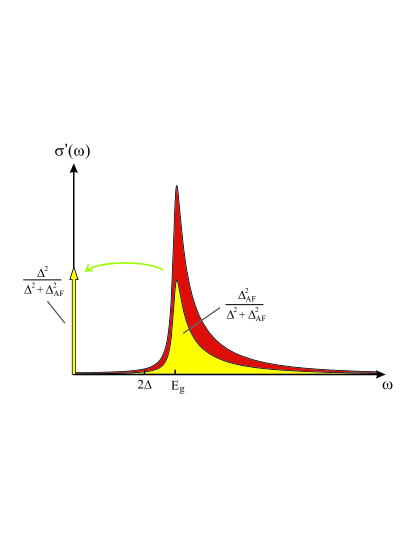
Figure 1: Transfer of optical spectral weight for a magnetic superconductor, considering particle-hole symmetry and a finite scattering rate $\tau^{-1}\simeq 0.07\Delta_{\mathrm{AF}}$. In the pure antiferromagnetic state (red), the spectrum has a peak at $E_{g}=2\Delta_{\mathrm{AF}}$ and no Drude peak. In the coexistence state (yellow), a fraction $\ \Delta^{2}/\left(\Delta_{\mathrm{AF}}^{2}+\Delta^{2}\right)$ of the total spectral weight of the antiferromagnetic phase is transferred to a finite Drude peak, while another fraction $\Delta_{\mathrm{AF}}^{2}/\left(\Delta_{\mathrm{AF}}^{2}+\Delta^{2}\right)$ stays at energies above the new optical gap $E_{g}=2\sqrt{\Delta_{\mathrm{AF}}^{2}+\Delta^{2}}$. Thus, a system without free carriers in the normal state acquires zero frequency spectral weight through transfer of weight over energies larger than $2\Delta$.

In the parent compounds $\mathrm{BaFe}_{2}\mathrm{As}_{2}$ and $\mathrm{SrFe}_{2}\mathrm{As}_{2}$, which do not show superconductivity, long range antiferromagnetic order below the Néel temperature $T_{N}$ leads to the formation of a mid-infrared (MIR) peakHu08 , with spectral weight being transferred to $\omega\simeq 2\Delta_{\mathrm{AF}}$ due to the opening of a spin density wave gap. Here $\Delta_{\mathrm{AF}}$ is the single-particle gap for momentum states that are Bragg scattered by the magnetic ordering vector (see figure 2). For $\mathrm{BaFe}_{2}\mathrm{As}_{2}$, $2\Delta_{\mathrm{AF}}\simeq 1000\mathrm{cm}^{-1}$ (i.e. $\Delta_{\mathrm{AF}}\simeq 62\mathrm{meV}$), yielding $\Delta_{\mathrm{AF}}/\left(k_{B}T_{N}\right)\simeq 5$, which is not unrealistic for itinerant antiferromagnets. For $T<T_{N}$, the low energy optical response of the parent compounds is characterized by the Drude form, Eq.(2), however with a significantly reduced plasma frequency $\omega_{p,\mathrm{AF}}^{2}\simeq\left(0.1-0.2\right)\omega_{p}^{2}$, where $\omega_{p}$ is the plasma frequency above $T_{N}$Hu08 . Finally, systematic investigations of $\sigma^{\prime}\left(\omega\right)$ in $\mathrm{Ba}(\mathrm{Fe}_{1-x}\mathrm{Co}_{x})_{2}\mathrm{As}_{2}$ as function of temperature and carrier concentration were performed in Refs.Uchida10 ; Lucarelli10 . Upon doping, the MIR peak gets weaker, consistent with the decrease of the ordered magnetic moment $M$ with dopingFernandes10 . Indeed, assuming $\Delta_{\mathrm{AF}}\propto M$ and using the results from Ref.Fernandes10 for the doping dependence of $M\left(T=0\right)$, one finds for doping concentrations where $T_{N}\simeq T_{c}$ that $\Delta_{\mathrm{AF}}\simeq\Delta$, strongly supporting the view that the same electrons that undergo Cooper pairing form the ordered moment. This is consistent with the recent analysisFernandes10 of the phase diagram of $\mathrm{Ba}(\mathrm{Fe}_{1-x}\mathrm{Co}_{x})_{2}\mathrm{As}_{2}$: neutron scattering experiments showed that magnetism and superconductivity compete strongly, to the extent that the staggered moment is suppressedPratt09 ; Christianson09 below $T_{c}$ and the magnetic phase boundary $T_{N}\left(x\right)$ is bent back towards smaller $x$-values for $T_{N}<T_{c}$. Theoretical arguments then demonstrate that this coexistence is only possible for an $s^{+-}$-pairing state. The optical properties in the regime of simultaneous magnetic and superconducting order are promising as they might reveal important information about the interplay between the superfluid condensate, the normal state Drude peak and the MIR peak.

In this paper we analyze the optical conductivity in the magnetically ordered phase as well as in the regime of simultaneous magnetic and superconducting order. Using parameters suitable to the description of the phase diagramFernandes10 of $\mathrm{Ba}(\mathrm{Fe}_{1-x}\mathrm{Co}_{x})_{2}\mathrm{As}_{2}$, we numerically obtain the optical spectrum below $T_{N}$. Due to the partial gapping of the Fermi surface in the itinerant antiferromagnetic state, we obtain a Drude peak in addition to a MIR peak at $\omega\simeq 2\Delta_{\mathrm{AF}}$, in qualitative agreement with the experimental data. Thus, our results give further strong evidence for the itinerant character of the magnetically ordered state.

As shown by nuclear magnetic resonance and muon spin rotation experimentsLaplace09 ; Julien09 ; Bernhard09 , antiferromagnetism and superconductivity coexist homogeneously in $\mathrm{Ba}(\mathrm{Fe}_{1-x}\mathrm{Co}_{x})_{2}\mathrm{As}_{2}$ for the doping range $0.035<x<0.059$. Recent tunnel diode resonator measurements showed that, in this regime, the $T=0$ superfluid density is reduced when compared to its value in the pure superconducting stateGordon10 . One might expect, at first glance, that such a reduction is due to the suppressed plasma frequency below $T_{N}$, and the inverse squared penetration depth $\lambda^{-2}$ is given by the reduced value $\omega_{p,\mathrm{AF}}^{2}/c^{2}$. In contrast to this expectation, we find that the superfluid condensate of a superconductor with magnetic long range order, while reduced compared to the case without magnetic order, has $\lambda^{-2}$ values that are significantly larger than $\omega_{p,\mathrm{AF}}^{2}/c^{2}$. In particular, we find a sizable condensate fraction even in the limit where $\omega_{p,\mathrm{AF}}^{2}=0$. By analytically investigating the simple but relevant limit of particle-hole symmetry, we demonstrate that, in the magnetically ordered superconducting state, spectral weight with energies $\omega\simeq 2\Delta_{\mathrm{AF}}$ is transferred from the MIR-peak into the singular $\delta\left(\omega\right)$ term of $\sigma^{\prime}\left(\omega\right)$, enhancing $n_{s}$ (see figure 1). This spectral weight is transferred from regions of the spectrum that can easily be larger than $2\Delta$, reflecting the fact that the rigidity of the superconducting ground state with respect to transverse current fluctuations, while smaller than in the paramagnet, is still larger than what the low frequency Drude weight would suggest.

Our results show that the superfluid density in a magnetic superconductor is not only related to the remaining electronic states of the magnetically reconstructed Fermi surface at $T=0$, but also to the transfer of spectral weight around the MIR peak. These conclusions are consistent with recent theoretical investigations from Vorontsov et al.Vorontsov10 showing that superconductivity is able to coexist with magnetism even when the reconstructed Fermi surface at $T=0$ is completely gapped.

The paper is organized as follows: in Section II we review the basic properties of the optical spectrum of classic superconductors. In Section III we present our results for the optical conductivity in the magnetically ordered phase of the iron arsenides. Section IV is devoted to the investigation of the optical spectrum of the coexistence state and its relationship to the superfluid density. Section V brings our conclusions and in Appendix A we present an explicit calculation of the penetration depth using an alternative approach.

II Optical conductivity in superconductors

Within the Kubo formalism the longitudinal optical conductivity is given by

$$\sigma\left(\omega\right)=\frac{i}{\omega+i0^{+}}\left(\Pi\left(\mathbf{q=0},\omega\right)+\frac{\omega_{p}^{2}}{4\pi}\right)$$ (5)

with longitudinal current-current correlation function

$$\Pi\left(\mathbf{q},\omega\right)=-i\int_{0}^{\infty}e^{i\omega t}\left\langle\left[j_{\alpha}\left(\mathbf{q,}t\right),j_{\alpha}\left(\mathbf{-q,}0\right)\right]_{-}\right\rangle dt.$$ (6)

where $j_{\alpha}$ is the $\alpha$-th component of the current operator. For the real part of the optical conductivity, we have:

$$\sigma^{\prime}\left(\omega\right)=\ D\delta\left(\omega\right)+\sigma_{\mathrm{reg}}^{\prime}\left(\omega\right),$$ (7)

with the regular contribution $\sigma_{\mathrm{reg}}\left(\omega\right)$, that does not contain a $\delta\left(\omega\right)$ contribution. From Eq.(5), it follows that the Drude weight $D$ of the optical conductivity is given by

$$D=\frac{1}{4}\left(\omega_{p}^{2}+4\pi\Pi\left(\mathbf{q=0},\omega\rightarrow 0\right)\right)$$ (8)

while the regular contribution is

$$\sigma_{\mathrm{reg}}^{\prime}\left(\omega\right)=-\frac{\mathrm{Im}\Pi\left(\mathbf{q=0},\omega\right)}{\omega}.$$ (9)

The current-current correlation function also determines the London penetration depth via

$$\lambda^{-2}=c^{-2}\left(\omega_{p}^{2}+4\pi\Pi\left(\mathbf{q\rightarrow 0},\omega=0\right)\right)$$ (10)

i.e. we consider the static current response at small but finite momentum, in distinction to the weight $D$ that measures the homogeneous ($\mathbf{q=0}$) response at small $\omega$. In general, the order of the limits $\mathbf{q=0}$, $\omega\rightarrow 0$ versus $\omega=0$, $\mathbf{q\rightarrow 0}$, matters and yields different results. Yet, in the case of a system with gapped excitation spectrum, it was shown in Ref.Scalapino93 that the order in which these limits are taken is irrelevant. Thus, in the case of a fully gapped superconductor, it follows generally that the Drude weight in the superconductor  

$$D=\frac{c^{2}}{4\lambda^{2}}$$ (11)

is determined by the penetration depth and thus by the superfluid condensate

$$n_{s}=\frac{m^{\ast}c^{2}}{4\pi e^{2}}\lambda^{-2}.$$ (12)

Formally, a contribution $D\neq 0$ in Eq.(7) is not a proof for superconductivity and may occur in a metallic system that is unable to relax its momentum. Then, the metal becomes a perfect conductor, where charges are freely accelerated by an external electric field. However, in a realistic system one always expects scattering events that allow for momentum relaxation. In case of a perfect conductor, such events broaden the singular Drude peak e.g.

$$\delta\left(\omega\right)\rightarrow\frac{1}{\pi}\frac{\tau}{1+\left(\omega\tau\right)^{2}}$$ (13)

with scattering time $\tau$. Thus, formally, $D=0$ and the Drude response becomes part of the regular contribution to the conductivity $\sigma_{\mathrm{reg}}^{\prime}\left(\omega\right)$. This is different for a superconductor, where scattering events may cause a reduction of the value of $D$ in Eq.(7) but do not change the $\delta\left(\omega\right)$-form of the zero frequency contribution. The Meissner effect requires  that $\omega_{p}^{2}>-4\pi\Pi\left(\mathbf{q\rightarrow 0},\omega=0\right)$. Together with the fact that the order of limits does not matter for a gapped systemScalapino93 , follows $D>0$, i.e. the $\delta\left(\omega\right)$-form is robust. This preservation of the singular $\omega=0$ response is a consequence of the unique rigidity of the superconductor with respect to transverse current fluctuations. Formally, this rigidity of the superconducting ground state is reflected by the smallness of $\left|\Pi\left(\mathbf{q\rightarrow 0},\omega=0\right)\right|$ compared to $\omega_{p}^{2}/\left(4\pi\right)$.

A quantitative determination of the penetration depth in a superconductor can be performed by analyzing the spectral weight transfer in $\sigma\left(\omega\right)$, and is expressed by the Ferrell-Glover-Tinkham (FGT) sum ruleFerrell58 ; Tinkham59 :

$$\lambda^{-2}=\frac{8}{c^{2}}\int_{0^{+}}^{\infty}\left(\sigma_{ns}^{\prime}\left(\omega\right)-\sigma_{sc}^{\prime}\left(\omega\right)\right)d\omega.$$ (14)

This sum rule relates $\lambda$ to the change of total spectral weight between the normal state ($ns$) and the superconducting ($sc$) state for $\omega>0$. It follows from the $f$-sum rule, Eq. (4), and the emergence of the $D\delta\left(\omega\right)$-term only below $T_{c}$. Thus, upon entering the superconducting state, spectral weight is transferred from finite frequencies to the $\delta$-function at $\omega=0$. We mention that for Eq.(14) to hold, one assumes that the expectation value of the optical mass $m^{\ast}$, i.e. the value of $\omega_{p}^{2}=4\pi e^{2}n/m^{\ast}$, is unaffected by the onset of superconductivity. In the FeAs superconductors, this seems to be the caseLi08 ; Uchida10 , in distinction to the evidence for violation of the FGT sum rule in cuprate superconductorsBasov05 .

III Optical spectrum in the itinerant antiferromagnetic phase

III.1 Microscopic model for competing magnetic and superconducting order

To develop a microscopic model of the interplay between superconductivity and magnetism, we use a few basic ingredients to describe the main features of the iron arsenidesFernandes10 : the electronic structure is characterized by two sets of Fermi surface sheets, a circular hole pocket around the center of the Brillouin zone and an elliptical electron pocket shifted by the magnetic ordering vector $\mathbf{Q}$. The non-interacting part $\mathcal{H}_{0}$ of the Hamiltonian is then given by

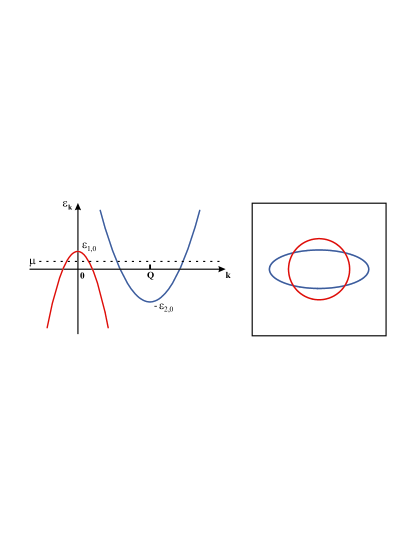
Figure 2: Schematic representation of the band structure considered here (left panel).The Fermi surface has an elliptical electron pocket (blue ellipse) displaced by the magnetic ordering vector $\mathbf{Q}$ from the circular hole pocket (red circle). In the right panel, we present the Fermi surface at zero doping. For simplicity, we displaced the centers of the bands to make them coincide.

$$\mathcal{H}_{0}=\sum_{\mathbf{k}\sigma}\left(\xi_{1,\mathbf{k}}c_{\mathbf{k}\sigma}^{\dagger}c_{\mathbf{k}\sigma}+\xi_{2,\mathbf{k}}d_{\mathbf{k}\sigma}^{\dagger}d_{\mathbf{k}\sigma}\right).$$ (15)

We consider only one hole band located in the center of the Brillouin zone with dispersion $\xi_{1,\mathbf{k}}$, and one electron band, shifted by $\mathbf{Q}$ from the hole band, with dispersion $\xi_{2,\mathbf{k}}$ (see figure 2):

$$\xi_{1,\mathbf{k}} = \varepsilon_{1,0}-\frac{k^{2}}{2m}-\mu$$ (16)

$$\xi_{2,\mathbf{k+Q}} = -\varepsilon_{2,0}+\frac{k_{x}^{2}}{2m_{x}}+\frac{k_{y}^{2}}{2m_{y}}-\mu,$$ (17)

A magnetic interaction $I$ and an interband pairing interaction $V$ lead to the possibility of antiferromagnetic order with antiferromagnetic gap

$$\Delta_{\mathrm{AF}}=\frac{I}{2}\sum_{\mathbf{k},\sigma}\sigma\left\langle c_{\mathbf{k}\sigma}^{\dagger}d_{\mathbf{k+Q}\sigma}\right\rangle$$ (18)

and superconductivity with coupled gap equations

$$\Delta_{2} = -\frac{V}{N}\sum_{\mathbf{k}}\left\langle c_{\mathbf{k}\uparrow}^{\dagger}c_{-\mathbf{k}\downarrow}^{\dagger}\right\rangle$$ (19)

$$\Delta_{1} = -\frac{V}{N}\sum_{\mathbf{k}}\left\langle d_{\mathbf{k+Q}\uparrow}^{\dagger}d_{-\mathbf{k}-\mathbf{Q}\downarrow}^{\dagger}\right\rangle.$$ (20)

For $V<0$, as it would be the case for phonon mediated superconductivity, one obtains the $s^{++}$ state ($\Delta_{1}\Delta_{2}>0$), whereas for $V>0$ it follows the unconventional sign-changing $s^{+-}$ state ($\Delta_{1}\Delta_{2}<0$). Introducing the Nambu operator $\Psi_{\mathbf{k}}=\left(c_{\mathbf{k\uparrow}},c_{-\mathbf{k\downarrow}}^{\dagger},d_{\mathbf{k+Q\uparrow}},d_{-\mathbf{k}-\mathbf{Q}\mathbf{\downarrow}}^{\dagger}\right)^{T}$, we consider the mean field Hamiltonian

$$H=\int_{\mathbf{k}}\Psi_{\mathbf{k}}^{\dagger}\widehat{\varepsilon}_{\mathbf{k}}\Psi_{\mathbf{k}}$$ (21)

with simultaneous antiferromagnetic and superconducting order. Here

$$\widehat{\varepsilon}_{\mathbf{k}}=\left(\begin{array}[]{cccc}\xi_{1,\mathbf{k}}&\Delta_{1}&\Delta_{\mathrm{AF}}&0\\ \Delta_{1}&-\xi_{1,\mathbf{k}}&0&\Delta_{\mathrm{AF}}\\ \Delta_{\mathrm{AF}}&0&\xi_{2,\mathbf{k+Q}}&\Delta_{2}\\ 0&\Delta_{\mathrm{AF}}&\Delta_{2}&-\xi_{2,\mathbf{k+Q}}\end{array}\right)$$ (22)

For details of this model, see Refs Fernandes10 ; Fernandes10_2 . Now, the $\mathbf{q=0}$ current-current correlation function is given by

$$\Pi_{\alpha\beta}\left(i\omega_{n}\right)=e^{2}T\sum_{\mathbf{k},m}\mathrm{tr}\left(\widehat{v}_{\mathbf{k}\alpha}\widehat{G}_{\mathbf{k}}\left(i\nu_{m}+i\omega_{n}\right)\widehat{v}_{\mathbf{k}\beta}\widehat{G}_{\mathbf{k}}\left(i\nu_{m}\right)\right)$$ (23)

with $\widehat{G}_{\mathbf{k}}^{-1}\left(i\omega_{n}\right)=i\omega_{n}\widehat{1}-\widehat{\varepsilon}_{\mathbf{k}}$ and the velocity matrix in Nambu space $\widehat{v}_{\mathbf{k}\alpha}=\partial/\partial k_{\alpha}\mathrm{diag}\left(\xi_{1,\mathbf{k}},\xi_{1,\mathbf{k}},\xi_{2,\mathbf{k+Q}},\xi_{2,\mathbf{k+Q}}\right)$. Here, the indices $\alpha$ and $\beta$ refer to Cartesian components of vectors, $\omega_{n}=2n\pi T$ is a bosonic Matsubara frequency and $\nu_{m}=(2m+1)\pi T$ is a fermionic Matsubara frequency.

III.2 Magnetically ordered phase without superconductivity

First, we investigate the optical properties of the pure antiferromagnetic state. In this case, one has $2\times 2$ matrices in Nambu space and the Green’s function is given by:

$$\widehat{G}_{s\mathbf{k}}\left(i\omega_{n}\right) = \left(i\omega_{n}-E_{1,\mathbf{k}}\right)^{-1}\left(i\omega_{n}-E_{2,\mathbf{k}}\right)^{-1}\times$$ (26)

$$\left(\begin{array}[]{cc}i\omega_{n}-\xi_{2,\mathbf{k+Q}}&-s\Delta_{\mathrm{AF}}\\ -s\Delta_{\mathrm{AF}}&i\omega_{n}-\xi_{1,\mathbf{k}}\end{array}\right)$$

where $s$ denotes the spin and $E_{a,\mathbf{k}}$, the quasiparticle energy:

$$E_{a,\mathbf{k}}=\left(\frac{\xi_{1,\mathbf{k}}+\xi_{2,\mathbf{k+Q}}}{2}\right)\pm\sqrt{\Delta_{\mathrm{AF}}^{2}+\left(\frac{\xi_{1,\mathbf{k}}-\xi_{2,\mathbf{k+Q}}}{2}\right)^{2}}$$ (27)

To evaluate the current-current correlation function, Eq. (23), we use the Kramers-Kronig relations:

$$\widehat{G}_{s\mathbf{k}}\left(i\omega_{n}\right)=-\int_{-\infty}^{\infty}\frac{d\Omega}{\pi}\frac{\mathrm{Im}\widehat{G}_{s\mathbf{k}}\left(\Omega+i0^{+}\right)}{i\omega_{n}-\Omega}$$ (28)

In order to obtain more realistic results, we replace one of the $i0^{+}$ convergence factors above by a finite single-particle lifetime $i\tau^{-1}$. Then, the real part of the conductivity is given only by the regular contribution (9). A straightforward calculation leads to:

$$\sigma_{\alpha\alpha}^{\prime}\left(\omega\right) = 2e^{2}v_{F,\alpha}^{2}\left(\frac{\tau^{-1}}{\omega^{2}+\tau^{-2}}\right)\sum_{a=1}^{2}\sum_{\mathbf{k}}\frac{f_{\alpha}\left(E_{a,\mathbf{k}},\omega\right)}{\left(E_{a,\mathbf{k}}-E_{\bar{a},\mathbf{k}}\right)}\times$$ (29)

$$\frac{\left(2\omega+E_{a,\mathbf{k}}-E_{\bar{a},\mathbf{k}}\right)}{\left(\omega+E_{a,\mathbf{k}}-E_{\bar{a},\mathbf{k}}\right)^{2}+\tau^{-2}}$$

where $\mathbf{v}_{F}$ is the hole-band Fermi velocity and:

$$f_{\alpha}\left(E_{a,\mathbf{k}},\omega\right) = \left[\frac{n_{F}\left(E_{a,\mathbf{k}}\right)-n_{F}\left(E_{a,\mathbf{k}}+\omega\right)}{\omega}\right]\times$$ (30)

$$\left(-\frac{2\Delta_{\mathrm{AF}}^{2}}{\bar{m}_{\alpha}}+\frac{C_{1,\mathbf{k}}^{(a)}}{\bar{m}_{\alpha}^{2}}+C_{2,\mathbf{k}}^{(a)}\right)$$

with $C_{i,\mathbf{k}}^{(a)}=\left(E_{a,\mathbf{k}}-\xi_{i,\mathbf{k}}\right)\left(E_{a,\mathbf{k}}+\omega-\xi_{i,\mathbf{k}}\right)$, Fermi function $n_{F}$ and relative electron-band mass $\bar{m}_{\alpha}=m_{\alpha}/m$. Here, we introduced the index $\bar{a}$ defined as $\bar{a}=2$ for $a=1$ and $\bar{a}=1$ for $a=2$.

In Ref. Fernandes10 , we introduced the band structure parameters that provide a good agreement between the model of the previous subsection and the neutron diffraction data on $\mathrm{Ba}(\mathrm{Fe}_{1-x}\mathrm{Co}_{x})_{2}\mathrm{As}_{2}$. Specifically, they are given by $\varepsilon_{1,0}=0.095$ eV, $\varepsilon_{2,0}=0.125$ eV, $m=1.32m_{\mathrm{electron}}$, $m_{x}=2m$, and $m_{y}=0.3m$, together with the electronic interaction $I=0.95$ eV and the assumption that each Co atom adds one extra electron. In this subsection, since we are only interested in the pure antiferromagnetic phase, we set $V=0$. In figure 3, we use these parameters to obtain the real part of the optical conductivity at approximately zero temperature and for different Co doping concentrations, with no superconductivity involved. Note that the only free parameter here is the single-particle lifetime $\tau$, which was chosen to be $\tau^{-1}=5.5$ meV for all doping concentrations. This is the same order of magnitude of the scattering rate associated with the narrow Drude peak observed in optical experimentsLucarelli10 .

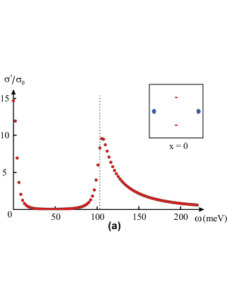
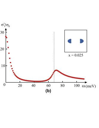
Figure 3: Real part of the optical conductivity $\sigma^{\prime}$ (in units of $\sigma_{0}=2\pi^{-1}\rho e^{2}v_{F,x}^{2}/\varepsilon_{0}$) as function of the frequency $\omega$ (in units of meV) at $T\approx 0$ for different Co doping concentrations: (a) $x=0$, (b) $x=0.025$, and (c) $x=0.057$. We use the band structure parameters that consistently describe the phase diagram of $\mathrm{Ba}(\mathrm{Fe}_{1-x}\mathrm{Co}_{x})_{2}\mathrm{As}_{2}$ (see main text for more details); only magnetic ordering is considered. The dashed gray line refers to the frequency $2\Delta_{\mathrm{AF}}$ and the inset shows the magnetically reconstructed Fermi surface (see figure 2).

Our objective here is not to describe all the details of the observed optical spectrum, which would require a description of all five Fe-3d orbitals (see, for example, Ref. Kaneshita09 ), but rather to understand its main features. From figure 3, we see that, in general, the optical spectrum in the antiferromagnetic phase has a Drude peak as well as a finite-frequency peak. The latter is located very close to $\omega\simeq 2\Delta_{\mathrm{AF}}$, and is associated with the opening of the spin density wave gap. As shown in the same figure, $\Delta_{\mathrm{AF}}$ only partially gaps the Fermi surface, resulting in a finite Drude peak proportional to $\tau$. Recall that, for nested bands and $\tau\rightarrow\infty$, the reconstructed Fermi surface is completely gapped and the optical conductivity in the magnetically ordered phase vanishes for $\omega<2\Delta_{\mathrm{AF}}$ (see Eq. 39 below for $\Delta=0$).

The existence of a peak at $2\Delta_{\mathrm{AF}}$, combined with the $f$-sum rule, Eq. (4), implies that the plasma frequency associated with the remaining Drude peak in the antiferromagnetic state must be smaller than the plasma frequency of the Drude peak in the paramagnetic phase, as seen experimentallyUchida10 (assuming that the optical mass is the same in both situations). Note that the theoretical value of $\Delta_{\mathrm{AF}}$ in the undoped sample is $\Delta_{\mathrm{AF}}\approx 51$ meV (Fig. 3a), which is very close to the value extracted from the measured optical spectrumHu08 . As doping increases and the magnitude of the gap decreases, the MIR peak gets weaker and moves towards lower frequencies (Fig. 3b), until it is almost completely masked by the Drude peak (Fig. 3c). These results are in general agreement with optical measurementsHu08 ; Uchida10 ; Lucarelli10 on $\mathrm{Ba}(\mathrm{Fe}_{1-x}\mathrm{Co}_{x})_{2}\mathrm{As}_{2}$, demonstrating the itinerant character of the magnetically ordered state in these compounds.

IV Optical spectrum in the magnetically ordered superconducting phase

So far we have considered only the magnetically ordered state. However, for $\mathrm{Ba}(\mathrm{Fe}_{1-x}\mathrm{Co}_{x})_{2}\mathrm{As}_{2}$, superconductivity coexists with antiferromagnetism at very low temperatures for $0.035<x<0.059$. In order to achieve a more transparent insight about the optical conductivity in the coexistence state, we investigate analytically the limit of particle-hole symmetry, where $\varepsilon_{0}\equiv\varepsilon_{1,0}=\varepsilon_{2,0}$, $m_{x}=m_{y}=m$ and $\mu=0$. In this case, $\xi_{\mathbf{k}}\equiv\xi_{1,\mathbf{k}}=-\xi_{2,\mathbf{k+Q}}$, implying that the hole and electron Fermi surfaces are identical (perfect nesting). In the case of $s^{+-}$-pairing we have

$$\widehat{\varepsilon}_{\mathbf{k}}=\xi_{\mathbf{k}}\tau_{3}\sigma_{3}+\Delta_{\mathrm{AF}}\tau_{0}\sigma_{1}+\Delta\tau_{1}\sigma_{z}$$ (31)

where $\Delta=\Delta_{1}=-\Delta_{2}$ and $\tau_{\alpha}$ and $\sigma_{\beta}$ are the Pauli matrices that act in Nambu and band space, respectively. In case of $s^{++}$-pairing, we replace $\sigma_{z}$ by $\sigma_{0}$ in the last term. Eq.(31) leads to the single particle Green’s function

$$\widehat{G}_{\mathbf{k}}\left(i\omega_{n}\right)=-\frac{i\omega_{n}\tau_{0}\sigma_{0}+\widehat{\varepsilon}_{\mathbf{k}}}{\omega_{n}^{2}+\Delta^{2}+\Delta_{\mathrm{AF}}^{2}+\xi_{\mathbf{k}}^{2}}.$$ (32)

At zero temperature the $\mathbf{q=0}$ current-current correlation function is:

$$\Pi\left(i\omega\right)=\frac{\omega_{p}^{2}}{2}\int\frac{d\Omega d\xi}{\left(4\pi\right)^{2}}\>\mathrm{tr}\left(\widehat{v}_{0}\widehat{G}_{\mathbf{k}}\left(i\omega+i\Omega\right)\widehat{v}_{0}\widehat{G}_{\mathbf{k}}\left(i\Omega\right)\right)$$ (33)

where $\widehat{v}_{0}=\tau_{0}\sigma_{z}$ contains the proper sign of the current vertex. Performing the trace over the band and Nambu degrees of freedom, we find

$$\Pi\left(\omega\right) = \frac{\omega_{p}^{2}}{8\pi^{2}}\int d\Omega d\xi\frac{\xi^{2}+\Delta^{2}-\Delta_{\mathrm{AF}}^{2}-\Omega\left(\omega+\Omega\right)}{\xi^{2}+\Delta_{\mathrm{AF}}^{2}+\Delta^{2}+\Omega^{2}}$$ (34)

$$\times\frac{1}{\xi^{2}+\Delta_{\mathrm{AF}}^{2}+\Delta^{2}+\left(\omega+\Omega\right)^{2}}$$

In the limit $\omega\rightarrow 0$ follows

$$\Pi\left(\omega\rightarrow 0\right)=-\frac{\omega_{p}^{2}}{4\pi}\frac{\Delta_{\mathrm{AF}}^{2}}{\Delta_{\mathrm{AF}}^{2}+\Delta^{2}}$$ (35)

and we obtain for the optical conductivity

$$D=\frac{\omega_{p}^{2}}{4}\frac{\Delta^{2}}{\Delta_{\mathrm{AF}}^{2}+\Delta^{2}}.$$ (36)

For the non-superconducting antiferromagnet ($\Delta=0$ but $\Delta_{\mathrm{AF}}\neq 0$) follows $D=0$. This is a consequence of perfect nesting that leads to a fully gapped antiferromagnetic state. In the non-magnetic superconductor ($\Delta_{\mathrm{AF}}=0$ but $\Delta\neq 0$) the current-current correlation function vanishes at $T=0$. Then, it follows $D=\omega_{p}^{2}/4$ and Eq.(11) yields the BCS result for the penetration depth $\lambda_{0}=\omega_{p}^{2}/c^{2}$. In the general case we obtain for the penetration depth

$$\lambda^{-2}=\lambda_{0}^{-2}\>\frac{\Delta^{2}}{\Delta_{\mathrm{AF}}^{2}+\Delta^{2}}$$ (37)

We point out that this result is the same as in the case of a charge density wave state coexisting with a conventional $s$-wave stateMachida84 . As shown in Appendix A, we obtain the same result for the penetration depth by explicitly analyzing Eq.(10), i.e. by first taking $\omega=0$ and then $\mathbf{q}\rightarrow 0$. In this context, the existence of a finite $\Pi\left(\omega=0,\mathbf{q}\rightarrow 0\right)$ at $T=0$ is related to the fact that one of the two coherence factors is not identically zero, in contrast to what happens for non-magnetic superconductors. Thus, the rigidity of the non-magnetic BCS ground state with respect to transverse current fluctuations is reduced in the magnetically ordered state.

Note that, formally, the coexistence between superconductivity and magnetism is only marginal for particle-hole symmetry, as we discussed elsewhereFernandes10 . Yet, small perturbations in both the chemical potential and the ellipticity of the electron band are able to place the system in the coexistence regimeFernandes10 ; Vavilov09 ; Vorontsov10 ; Fernandes10_2 . Following Refs. Vavilov09 ; Vorontsov10 , we can investigate the effect of these small perturbations on our result for the penetration depth (37) by considering the perturbed band structure $\xi_{2,\mathbf{k}\mathbf{+Q}}=-\xi_{1,\mathbf{k}}-2\delta_{\varphi}$, with $\delta_{\varphi}=\delta_{0}+\delta_{2}\cos 2\varphi$ such that $\delta_{0}=\mu+\frac{k_{F}^{2}}{4}\left(\frac{1}{m}-\frac{m_{x}+m_{y}}{2m_{x}m_{y}}\right)$ and $\delta_{2}=\frac{k_{F}^{2}}{8}\left(\frac{m_{x}-m_{y}}{m_{x}m_{y}}\right)$. Here, $\varphi$ is the angle on the elliptical electron pocket. A straightforward calculation leads to:

$$\lambda^{-2}\approx\lambda_{0}^{-2}\>\frac{\Delta^{2}}{\Delta_{\mathrm{AF}}^{2}+\Delta^{2}}\left[1+\frac{4\Delta_{\mathrm{AF}}^{2}}{3\left(\Delta_{\mathrm{AF}}^{2}+\Delta^{2}\right)^{2}}\left\langle\delta_{\varphi}^{2}\right\rangle\right]$$ (38)

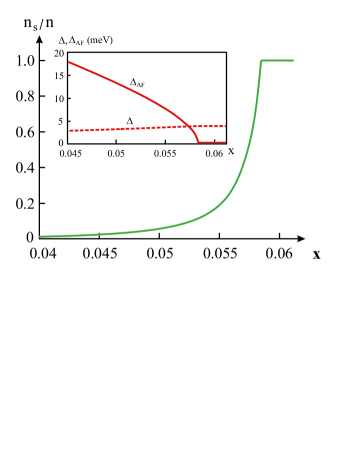
Figure 4: Ratio of the superfluid condensate $n_{s}$ and the electron density $n$ with parameters relevant for $\mathrm{Ba}(\mathrm{Fe}_{1-x}\mathrm{Co}_{x})_{2}\mathrm{As}_{2}$ in the clean limit, as function of $x$ and for $T=0$. For $x\lesssim 0.059$ simultaneous antiferromagnetic and superconducting order sets in while for $x\gtrsim 0.059$ no long range magnetic order exists. The inset shows the $T=0$ values of $\Delta$ (dashed red line) and $\Delta_{\mathrm{AF}}$ (solid red line) as function of $x$, according to the theory of Ref. Fernandes10 . For simplicity we consider the particle-hole symmetry expression (37) and use the value of the SC gap referent to the electron band.

with $\left\langle\delta_{\varphi}^{2}\right\rangle=\delta_{0}^{2}+\delta_{2}^{2}/2$. Thus, both perturbations in the chemical potential and in the ellipticity lead to a decrease in the penetration depth, i.e. to an increase in the value of $D$. Therefore, we can interpret the particle-hole symmetric result (37) as an “upper-bound” for $\lambda$. With this in mind, even though the band structure of the pnictides is not particle-hole symmetric, it is instructive to substitute in Eq. (37) the $T=0$ values of $\Delta$ and $\Delta_{\mathrm{AF}}$ obtained by numerically solving the gap equations with the band structure parameters of $\mathrm{Ba}(\mathrm{Fe}_{1-x}\mathrm{Co}_{x})_{2}\mathrm{As}_{2}$ (see Section III). The results are displayed in figure 4. Remarkably, similar values for the relative increase of $\lambda_{T=0}$ have been recently measured by Gordon et al.Gordon10 along the coexistence region of $\mathrm{Ba}(\mathrm{Fe}_{1-x}\mathrm{Co}_{x})_{2}\mathrm{As}_{2}$ using the tunnel diode resonator technique.

Next, we analyze the optical conductivity at finite frequencies. To this end, we evaluate the integrations in Eq.(34) and perform the analytical continuation to the real frequency axis, $i\omega\rightarrow\omega+i0^{+}$, obtaining:

$$\sigma_{reg}^{\prime}\left(\omega\right)=\left\{\begin{array}[]{cc}0&\omega<E_{g}\\ \frac{\omega_{p}^{2}}{2\omega^{2}}\frac{\Delta_{\mathrm{AF}}^{2}}{\sqrt{\omega^{2}-E_{g}^{2}}}&\omega\geq E_{g}\end{array}\right.$$ (39)

with the optical gap

$$E_{g}=2\sqrt{\Delta_{\mathrm{AF}}^{2}+\Delta^{2}}$$ (40)

In the normal state, $\Delta=0$ and the optical conductivity is nonzero only for $\omega>$ $2\Delta_{\mathrm{AF}}$. Entering the superconducting state, it follows for $\Delta<\Delta_{\mathrm{AF}}$ that there is no spectral weight in the normal state for $\omega<2\Delta$. Thus, the finite penetration depth obtained in Eq.(37) must be due to the transfer of spectral weight that involves energies above $2\Delta$. Indeed, analyzing the remaining high frequency spectral weight, we find from Eq.(39) that

$$2\int_{E_{g}}^{\infty}\sigma_{reg}^{\prime}\left(\omega\right)d\omega=\frac{\omega_{p}^{2}}{4}\frac{\Delta_{\mathrm{AF}}^{2}}{\Delta_{\mathrm{AF}}^{2}+\Delta^{2}}$$ (41)

where the factor of $2$ accounts for negative frequencies. Thus, the total weight of the non-superconducting antiferromagnet splits in two parts with ratio $\left(\Delta/\Delta_{\mathrm{AF}}\right)^{2}$. Below $T_{c}$ a fraction $\ \Delta^{2}/\left(\Delta_{\mathrm{AF}}^{2}+\Delta^{2}\right)$ is transferred to $\omega=0$ to yield Meissner screening and a finite penetration depth. In addition, the fraction $\Delta_{\mathrm{AF}}^{2}/\left(\Delta_{\mathrm{AF}}^{2}+\Delta^{2}\right)$ remains at energies above the optical gap $E_{g}$, as illustrated in figure 1. Here we use the fact that $E_{g}$ of the non-superconducting antiferromagnetic state and of the state with $\Delta$ and $\Delta_{\mathrm{AF}}$ finite is essentially the same due to the reduced ordered moment below $T_{c}$, see Ref.Fernandes10 .

Analogously, one can rationalize this result using Ferrell-Glover-Tinkham (FGT) sum rule, Eq. (14). By calculating the difference of spectral weight between the non-superconducting state and the superconducting state with the same value of $\Delta_{\mathrm{AF}}$, we obtain exactly the Drude weight $D$:

$$2\int_{0^{+}}^{\infty}\left[\sigma_{reg}^{\prime}\left(\omega,\Delta_{\mathrm{AF}},\Delta=0\right)-\sigma_{reg}^{\prime}\left(\omega,\Delta_{\mathrm{AF}},\Delta\right)\right]d\omega$$

$$=\frac{\omega_{p}^{2}}{4}\frac{\Delta^{2}}{\Delta_{\mathrm{AF}}^{2}+\Delta^{2}}$$ (42)

Our analysis for particle-hole symmetry clearly shows that, in a magnetic superconductor, the transfer of spectral weight to the Drude peak below $T_{c}<T_{N}$ is not from $\omega<2\Delta$, but from higher frequencies $\omega<2\sqrt{\Delta_{\mathrm{AF}}^{2}+\Delta^{2}}$. Therefore, analyzing our results for the optical conductivity of the pure magnetic phase (figure 3), as well as the experimental optical spectrum, the superfluid condensate is formed not only by the reduced remaining Drude peak but also by the significant portion of spectral weight associated with the MIR peak. More importantly, even in the absence of a remaining Drude peak in the pure magnetic state at $T=0$, spectral weight can be transferred to a $\delta\left(\omega\right)$-term below $T_{c}$, yielding a finite superfluid density.

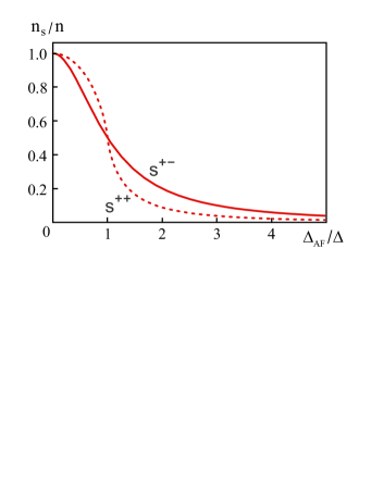
Figure 5: Ratio of the superfluid density $n_{s}$ and the electron density $n$ as function of the antiferromagnetic gap $\Delta_{\mathrm{AF}}$ (in units of the superconducting gap $\Delta$) for $s^{++}$-pairing (dashed line) and $s^{+-}$-pairing (solid line) at $T=0$.

Let us briefly discuss the situation for $s^{++}$-superconductivity and particle-hole symmetric bands. Similar calculations lead to the $T=0$ penetration depth

$$\lambda^{-2}=\lambda_{0}^{-2}\frac{2\Delta\Delta_{\mathrm{AF}}+\left(\Delta_{\mathrm{AF}}^{2}-\Delta^{2}\right)\ln\left|\frac{\Delta_{\mathrm{AF}}-\Delta}{\Delta_{\mathrm{AF}}+\Delta}\right|}{4\Delta\Delta_{\mathrm{AF}}}.$$ (43)

Correspondingly, the high frequency contribution has the total weight $1-\left(\lambda_{0}/\lambda\right)^{2}$ . In figure 5 we plot the superfluid density $n_{s}\left(\Delta,\Delta_{\mathrm{AF}}\right)$ as function of $\Delta_{\mathrm{AF}}/\Delta$ for $s^{++}$ and $s^{+-}$-pairing. We see that for $\Delta_{\mathrm{AF}}<\Delta$ holds that $n_{s}$ is larger for $s^{++}$-pairing compared to $s^{+-}$, while the opposite is true for $\Delta_{\mathrm{AF}}>\Delta$. Qualitatively, the two behaviors are not very different and would not provide a sharp criterion to identify the symmetry of the pairing state in the iron arsenides. Yet, previous analysisFernandes10 ; Fernandes10_2 ; Vorontsov10 demonstrated that the conventional $s^{++}$ state is unable to coexist with itinerant magnetism in the pnictides.

V Conclusions

In conclusion, we analyzed the optical conductivity of both an itinerant antiferromagnetic state and a magnetically ordered superconductor. For the pure magnetic phase, using the parameters associated to the phase diagramFernandes10 ; Fernandes10_2 of $\mathrm{Ba}(\mathrm{Fe}_{1-x}\mathrm{Co}_{x})_{2}\mathrm{As}_{2}$, we were able to identify the main features observed in the experimental optical spectrumHu08 ; Uchida10 ; Lucarelli10 . In particular, for the undoped compound, we found a reduced Drude peak associated to the remaining reconstructed parts of the Fermi surface, as well as a mid-infrared (MIR) peak at $\omega\simeq 2\Delta_{\mathrm{AF}}\approx 51$ meV, associated to the gap opened at momentum $\mathbf{k_{0}}$ that are Bragg scattered by the magnetic ordering vector $\mathbf{Q}$, i.e. $\xi_{1,\mathbf{k}_{0}}=\xi_{2,\mathbf{k_{0}+Q}}$. Upon doping, the spin density wave gap is reduced and, consequently, the MIR peak becomes weaker and more masked by the Drude peak.

The experimentally observed optical conductivity has other particular features that are not contemplated by our two-band based model, such as high-frequency interband transitions, a seemingly doping-independent incoherent contribution with a rather long tail, other possible low-weight Drude-like peaks at finite frequenciesUchida10 ; Lucarelli10 and, of course, the origin of the scattering processes that lead to a finite lifetime $\tau$. Clearly, a detailed description of the optical spectrum has to take into account the effects of the other bands that do not participate in the spin density wave stateKaneshita09 , and possibly the role played by different orbitals that cross the Fermi level. Yet, our simplified model that provides a very satisfactory descriptionFernandes10 of the phase diagram of $\mathrm{Ba}(\mathrm{Fe}_{1-x}\mathrm{Co}_{x})_{2}\mathrm{As}_{2}$, is able to correctly capture not only the main qualitative features of the spectrum, but also the order of magnitude of the frequency associated to the MIR peak.

Most interestingly, our results clarify how spectral weight is transferred in magnetic superconductors below the superconducting transition temperature, even in case where the Fermi surface of the ordered magnet is fully gapped. In classical superconductors, only the spectral weight below the optical gap $E_{g}=2\Delta$ is transferred to the Drude peak. However, in the case where itinerant magnetism is also present and particle-hole symmetry holds, the optical gap is given by $E_{g}=2\sqrt{\Delta_{\mathrm{AF}}^{2}+\Delta^{2}}$, involving energies that can potentially be much larger than the superconducting gap. Thus, in the regime where magnetism and superconductivity coexist in the iron arsenides, the remaining Drude peak of the antiferromagnetic phase, whose plasma frequency can be significantly smaller than the plasma frequency of the paramagnetic state, is not the only origin for the value of the superfluid condensate. Instead, spectral weight associated to the higher-frequency MIR peak is transferred to the $\delta$-function at $\omega=0$, enhancing the superfluid condensate. Yet, this superfluid density is always smaller than its value in the non-magnetic superconducting phase, in agreement with experimentsGordon10 .

This transfer of optical spectral weight is a consequence of the unique rigidity of the superconductor with respect to transverse current fluctuations. It implies that, even in the limit where the pure $T=0$ antiferromagnetic phase has no Drude peak, it is still possible to obtain a finite superfluid density below $T_{c}$. The superfluid density of the coexistence state is not only associated to electronic states from the remaining Fermi surface, what allows the superconducting transition to take place even when a Fermi surface would not be present in the magnetically ordered state. This non-trivial observation is corroborated by recent calculations of Vorontsov et al.Vorontsov10 , that found coexisting itinerant magnetism and $s^{+-}$ superconductivity in cases where the reconstructed Fermi surface would be completely gapped at $T=0$. As they pointed out, in these situations both the antiferromagnetic and superconducting phases are “effectively attractive” and cooperate to form the coexistence state.

We are grateful to R. Gordon and R.Prozorov for helpful discussions and for sharing their penetration depth data prior to publication. This research was supported by the Ames Laboratory, operated for the U.S. Department of Energy by Iowa State University under Contract No. DE-AC02-07CH11358.

Appendix A Calculation of the penetration depth in the coexistence region

Using Kramers-Kronig relations, the current-current correlation function (23) at finite momentum and finite frequency can be written as:

$$\Pi_{\alpha\beta}\left(\mathbf{q},i\omega_{n}\right)=e^{2}T\sum_{\mathbf{k},\nu_{m}}\int_{-\infty}^{\infty}\frac{d\nu}{\pi}\int_{-\infty}^{\infty}\frac{d\nu^{\prime}}{\pi}\mathrm{tr}\left(\widehat{v}_{\mathbf{k+q}\alpha}\frac{\mathrm{Im}\widehat{G}_{\mathbf{k}+\mathbf{q}}\left(\nu^{\prime}+i0^{+}\right)}{i\nu_{m}+i\omega_{n}-\nu^{\prime}}\widehat{v}_{\mathbf{k}\beta}\frac{\mathrm{Im}\widehat{G}_{\mathbf{k}+\mathbf{q}}\left(\nu+i0^{+}\right)}{i\nu_{m}-\nu}\right)$$ (44)

It is straightforward to evaluate the Matsubara sum. Setting $\omega_{n}=0$ yields:

$$\Pi_{\alpha\beta}\left(\mathbf{q},\omega=0\right)=e^{2}\sum_{\mathbf{k}}\int_{-\infty}^{\infty}\frac{d\nu}{\pi}\int_{-\infty}^{\infty}\frac{d\nu^{\prime}}{\pi}\left[\frac{n_{F}\left(\nu\right)-n_{F}\left(\nu^{\prime}\right)}{\nu-\nu^{\prime}}\right]\mathrm{tr}\left(\widehat{v}_{\mathbf{k+q}\alpha}\mathrm{Im}\widehat{G}_{\mathbf{k}+\mathbf{q}}\left(\nu^{\prime}+i0^{+}\right)\widehat{v}_{\mathbf{k}\beta}\mathrm{Im}\widehat{G}_{\mathbf{k}+\mathbf{q}}\left(\nu+i0^{+}\right)\right)$$ (45)

where $n_{F}$ is the Fermi function. The imaginary part of the Green’s function can be calculated directly from Eq. (32):

$$\widehat{G}_{\mathbf{k}}\left(\nu+i0^{+}\right)=\frac{\nu\tau_{0}\sigma_{0}+\widehat{\varepsilon}_{\mathbf{k}}}{2E_{\mathbf{k}}}\left(\frac{1}{\nu-E_{\mathbf{k}}+i0^{+}}-\frac{1}{\nu+E_{\mathbf{k}}+i0^{+}}\right)$$ (46)

where we defined the positive excitation energy $E_{\mathbf{k}}=\sqrt{\xi_{\mathbf{k}}^{2}+\Delta_{\mathrm{AF}}^{2}+\Delta^{2}}$. It follows that:

$$\mathrm{Im}\widehat{G}_{\mathbf{k}}\left(\nu+i0^{+}\right)=-\frac{\pi\left(\nu\tau_{0}\sigma_{0}+\widehat{\varepsilon}_{\mathbf{k}}\right)}{2E_{\mathbf{k}}}\left[\delta\left(\omega-E_{\mathbf{k}}\right)-\delta\left(\omega+E_{\mathbf{k}}\right)\right]$$ (47)

Substituting Eq. (47) in the expression (45), we can evaluate the frequency integrals as well as the trace in Nambu space. In the limit of small momentum, we obtain:

$$\Pi_{\alpha\beta}\left(\mathbf{q}\rightarrow 0,\omega=0\right) = \lim_{\mathbf{q}\rightarrow 0}\sum_{\mathbf{k}}2e^{2}v_{\mathbf{k}}^{\alpha}v_{\mathbf{k}}^{\beta}\left\{\left[\frac{n_{F}\left(E_{\mathbf{k}}\right)-n_{F}\left(E_{\mathbf{k}+\mathbf{q}}\right)}{E_{\mathbf{k}}-E_{\mathbf{k}+\mathbf{q}}}\right]\left(1+\frac{\xi_{\mathbf{k}}\xi_{\mathbf{k}+\mathbf{q}}+\Delta^{2}-\Delta_{\mathrm{AF}}^{2}}{E_{\mathbf{k}}E_{\mathbf{k}+\mathbf{q}}}\right)\right.$$ (48)

$$\left.+\left[\frac{n_{F}\left(E_{\mathbf{k}}\right)-n_{F}\left(-E_{\mathbf{k}+\mathbf{q}}\right)}{E_{\mathbf{k}}+E_{\mathbf{k}+\mathbf{q}}}\right]\left(1-\frac{\xi_{\mathbf{k}}\xi_{\mathbf{k}+\mathbf{q}}+\Delta^{2}-\Delta_{\mathrm{AF}}^{2}}{E_{\mathbf{k}}E_{\mathbf{k}+\mathbf{q}}}\right)\right\}$$

yielding, for a two-dimensional isotropic superconductor:

$$\Pi_{\alpha\beta}\left(\mathbf{q}\rightarrow 0,\omega=0\right) = -v_{F}^{2}e^{2}\delta_{\alpha\beta}\sum_{\mathbf{k}}\left[2\left(-\frac{\partial n_{F}}{\partial E_{\mathbf{k}}}\right)\left(1-\frac{\Delta_{\mathrm{AF}}^{2}}{E_{\mathbf{k}}^{2}}\right)+\frac{\Delta_{\mathrm{AF}}^{2}}{E_{\mathbf{k}}^{3}}\tanh\left(\frac{\beta E_{\mathbf{k}}}{2}\right)\right]$$ (49)

We introduce the density of states $\rho$ and take $T=0$, obtaining:

$$\Pi_{\alpha\beta}\left(\mathbf{q}\rightarrow 0,\omega=0\right)=-\rho v_{F}^{2}e^{2}\delta_{\alpha\beta}\int_{-\infty}^{\infty}d\xi\left[2\delta\left(\sqrt{\xi^{2}+\Delta^{2}+\Delta_{\mathrm{AF}}^{2}}\right)\left(1-\frac{\Delta_{\mathrm{AF}}^{2}}{\xi^{2}+\Delta^{2}+\Delta_{\mathrm{AF}}^{2}}\right)+\frac{\Delta_{\mathrm{AF}}^{2}}{\left(\xi^{2}+\Delta^{2}+\Delta_{\mathrm{AF}}^{2}\right)^{3/2}}\right]$$ (50)

For $\Delta\neq 0$ or $\Delta_{\mathrm{AF}}\neq 0$ the first term vanishes, whereas the second one gives:

$$\Pi_{\alpha\beta}\left(\mathbf{q}\rightarrow 0,\omega=0\right)=-2\rho v_{F}^{2}e^{2}\delta_{\alpha\beta}\left(\frac{\Delta_{\mathrm{AF}}^{2}}{\Delta^{2}+\Delta_{\mathrm{AF}}^{2}}\right)$$ (51)

which leads to the same result as Eq. (37) from the main text. Notice, from Eq. (48), that the non-zero value assumed by the current-current correlation function at $T=0$ is due to the coherence factor $\left(1-\frac{\xi_{\mathbf{k}}\xi_{\mathbf{k}+\mathbf{q}}+\Delta^{2}-\Delta_{\mathrm{AF}}^{2}}{E_{\mathbf{k}}E_{\mathbf{k}+\mathbf{q}}}\right)$. For a non-magnetic superconductor, this term goes to zero as $\mathbf{q}\rightarrow 0$ for any temperature; then, the only contribution to the current-current correlation function comes from the usual coherence factor $\left(1+\frac{\xi_{\mathbf{k}}\xi_{\mathbf{k}+\mathbf{q}}+\Delta^{2}-\Delta_{\mathrm{AF}}^{2}}{E_{\mathbf{k}}E_{\mathbf{k}+\mathbf{q}}}\right)$, whose prefactor vanishes at $T=0$ due to the existence of a gap in the quasiparticle energy spectrum. In both coherence factors, the relative minus sign between $\Delta^{2}$ and $\Delta_{\mathrm{AF}}^{2}$ is a result of the fact that while $\xi$ and $\Delta$ change from one Fermi surface sheet to the other, $\Delta_{\mathrm{AF}}$ stays the same. Therefore, the change in the penetration depth cannot be attributed to a change only in the density of states, in accordance to our analysis of the finite frequency optical spectrum.

References

- (1) D. C. Mattis and J. Bardeen, Phys. Rev. 111, 412 (1958).
- (2) R. A. Ferrell and R. E. Glover, III, Phys. Rev. 109, 1398 (1958).
- (3) M. Tinkham and R. A. Ferrell, Phys. Rev. Lett. 2, 331 (1959).
- (4) J. Bardeen, L. N. Cooper and J. R. Schrieffer, Physical Review 106, 162 (1957).
- (5) A. A. Abrikosov, L. P. Gor’kov, and I. E. Dzyaloshinskii, Quantum field theoretical methods in statistical physics, ed., Pergamon, (1965).
- (6) D.N. Basov and T. Timusk, Rev. Mod. Phys. 77, 721 (2005).
- (7) M. R. Norman, A. V. Chubukov, E. van Heumen, A. B. Kuzmenko, and D. van der Marel, Phys. Rev. B 76, 220509(R) (2007).
- (8) J. P. Carbotte, E. Schachinger, and D. N. Basov, Nature (London) 401, 354 (1999).
- (9) Ar. Abanov, A. V. Chubukov and J. Schmalian, Phys. Rev. B 63, 180510(R) (2001).
- (10) Ar. Abanov, A. V. Chubukov and J. Schmalian, J. Electron Spectrosc. Relat. Phenom. 117-118, 129 (2001).
- (11) E. van Heumen, E. Muhlethaler, A. B. Kuzmenko, H. Eisaki, W. Meevasana, M. Greven, and D. van der Marel, Phys. Rev. B 79, 184512 (2009).
- (12) Y. Kamihara, T.Watanabe, M. Hirano, and H. Hosono, J. Am. Chem. Soc. 130, 3296 (2008).
- (13) M. Rotter, M. Tegel, and D. Johrendt, Phys. Rev. Lett. 101, 107006 (2008).
- (14) I.I. Mazin, D.J. Singh, M.D. Johannes, M.H. Du, Phys. Rev. Lett. 101, 057003 (2008).
- (15) A. D. Christianson, E. A. Goremychkin, R. Osborn, S. Rosenkranz, M. D. Lumsden, C. D. Malliakas, I. S. Todorov, H. Claus, D. Y. Chung, M. G. Kanatzidis, R. I. Bewley, and T. Guidi, Nature 456, 930 (2008).
- (16) R. M. Fernandes, D. K. Pratt, W. Tian, J. Zarestky, A. Kreyssig, S. Nandi, M.-G. Kim, A. Thaler, N.Ni, P. C. Canfield, R. J. McQueeney, J. Schmalian, and A. I. Goldman, Phys. Rev. B 81, 140501(R) (2010).
- (17) C. T. Chen, C. C. Tsuei, M. B. Ketchen, Z. A. Ren, Z. X. and Zhao, Nature Phys. 6, 260 (2010).
- (18) G. Li, W. Z. Hu, J. Dong, Z. Li, P. Zheng, G. F. Chen, J. L. Luo, and N. L. Wang, Phys. Rev. Lett. 101, 107004 (2008).
- (19) W. Z. Hu, J. Dong, G. Li, Z. Li, P. Zheng, G. F. Chen, J. L. Luo, and N. L. Wang, Phys. Rev. Lett. 101, 257005 (2008).
- (20) F. Pfuner, J. G. Analytis, J.-H. Chu, I. R. Fisher and L. Degiorgi, European Physical Journal B 67, 513 (2009).
- (21) D. Wu, N. Barišić, P. Kallina, A. Faridian, B. Gorshunov, N. Drichko, L. J. Li, X. Lin, G. H. Cao, Z. A. Xu, N. L. Wang, and M. Dressel, Phys. Rev. B 81, 100512(R) (2010).
- (22) M. Nakajima, S. Ishida, K. Kihou, Y. Tomioka, T. Ito, Y. Yoshida, C. H. Lee, H. Kito, A. Iyo, H. Eisaki, K. M. Kojima, and S. Uchida, Phys. Rev. B 81, 104528 (2010).
- (23) B. Gorshunov, D. Wu, A. A. Voronkov, P. Kallina, K. Iida, S. Haindl, F. Kurth, L. Schultz, B. Holzapfel, and M. Dressel, Phys. Rev. B 81, 060509(R) (2010).
- (24) E. van Heumen, Y. Huang, S. de Jong, A.B. Kuzmenko, M.S. Golden, and D. van der Marel, arXiv:0912.0636 (2009).
- (25) K. W. Kim, M. Rössle, A. Dubroka, V. K. Malik, T. Wolf, and C. Bernhard, arXiv:0912.0140 (2009).
- (26) A. Lucarelli, A. Dusza, F. Pfuner, P. Lerch, J.G. Analytis, J.-H. Chu, I.R. Fisher, L. Degiorgi, arXiv:1004.3022 (2010).
- (27) R. T. Gordon, H. Kim, N. Salovich, R. W. Giannetta, R. M. Fernandes, V. G. Kogan, T. Prozorov, S. L. Bud’ko, P. C. Canfield, M. A. Tanatar, and R. Prozorov, arXiv:1006.2068 (2010).
- (28) D. K. Pratt, W. Tian, A. Kreyssig, J. L. Zarestky, S. Nandi, N. Ni, S. L. Bud’ko, P. C. Canfield, A. I. Goldman, and R. J. McQueeney, Phys. Rev. Lett. 103, 087001 (2009).
- (29) A. D. Christianson, M. D. Lumsden, S. E. Nagler, G. J. MacDougall, M. A. McGuire, A. S. Sefat, R. Jin, B. C. Sales, and D. Mandrus, Phys. Rev. Lett. 103, 087002 (2009).
- (30) Y. Laplace, J. Bobroff, F. Rullier-Albenque, D. Colson, and A. Forget, Phys. Rev. B 80, 140501(R) (2009)
- (31) M.-H. Julien, H. Mayaffre, M. Horvatić, C. Berthier, X. D. Zhang, W. Wu, G. F. Chen, N. L. Wang and J. L. Luo, Europhys. Lett. 87, 37001 (2009).
- (32) C. Bernhard, A. J. Drew, L. Schulz, V. K. Malik, M. Rössle, Ch. Niedermayer, Th. Wolf, G. D. Varma, G. Mu, H.-H. Wen, H. Liu, G. Wu, and X. H. Chen, New J. Phys. 11, 055050 (2009).
- (33) A. B. Vorontsov, M. G.Vavilov, and A. V.Chubukov, arXiv:1003.2389 (2010).
- (34) D. J. Scalapino, S. R. White, and S. Zhang, Phys. Rev. B 47, 7995 (1993).
- (35) R. M. Fernandes and J. Schmalian, arXiv:1005.2437 (2010).
- (36) E. Kaneshita, T. Morinari, and T. Tohyama, Phys. Rev. Lett. 103, 247202 (2009).
- (37) K. Machida, J. Phys. Soc. Jpn. 53, 712 (1984).
- (38) M. G. Vavilov, A. V. Chubukov, and A. B. Vorontsov, arXiv:0912.3556 (2009).