Inertial waves in rotating bodies: a WKBJ formalism for inertial modes and a comparison with numerical results

Abstract

Inertial waves governed by Coriolis forces may play an important role in several astrophysical settings, such as eg. tidal interactions, which may occur in extrasolar planetary systems and close binary systems, or in rotating compact objects emitting gravitational waves. Additionally, they are of interest in other research fields, eg. in geophysics.

However, their analysis is complicated by the fact that in the inviscid case the normal mode spectrum is either everywhere dense or continuous in any frequency interval contained within the inertial range. Moreover, the equations governing the corresponding eigenproblem are, in general, non-separable.

In this paper we develop a consistent WKBJ formalism, together with a formal first order perturbation theory for calculating the properties of the normal modes of a uniformly rotating coreless body (modelled as a polytrope and referred hereafter to as a planet) under the assumption of a spherically symmetric structure. The eigenfrequencies, spatial form of the associated eigenfunctions and other properties we obtained analytically using the WKBJ eigenfunctions are in good agreement with corresponding results obtained by numerical means for a variety of planet models even for global modes with a large scale distribution of perturbed quantities. This indicates that even though they are embedded in a dense spectrum, such modes can be identified and followed as model parameters changed and that first order perturbation theory can be applied.

This is used to estimate corrections to the eigenfrequencies as a consequence of the anelastic approximation, which we argue here to be small when the rotation frequency is small. These are compared with simulation results in an accompanying paper with a good agreement between theoretical and numerical results.

The results reported here may provide a basis of theoretical investigations of inertial waves in many astrophysical and other applications, where a rotating body can be modelled as a uniformly rotating barotropic object, for which the density has, close to its surface, an approximately power law dependence on distance from the surface.

1 Introduction

In astrophysical applications inertial waves that can exist in rotating bodies may be excited by several different physical mechanisms, most notably through tidal perturbation by a companion (eg. Papaloizou & Pringle 1981, hereafter PP) or in the case of compact objects through secular instability arising through gravitational wave losses (eg. Chandrasekhar 1970, Friedman & Schutz 1978, Andersson 1998, Friedman $\&$ Morsink 1998). They also can play a role in other physical systems. For example, they can also be excited by several mechanisms in the Earth’s fluid core with possible detection being announced (Aldridge $\&$ Lumb 1987).

For rotating planets and stars that have a barotropic equation of state these wave modes are governed by Coriolis forces and so have oscillation periods that are comparable to the rotation period. They are accordingly readily excited by tidal interaction with a perturbing body when the characteristic time associated with the orbit is comparable to the rotation period, which is expected naturally when the rotation period and orbit become tidally coupled. They may then play an important role in governing the secular orbital evolution of the system.

Inertial modes excited in close binary systems in circular orbit were considered by PP and Savonije & Papaloizou (1997). Wu (2005)a,b considered the excitation of inertial modes in Jupiter as a result of tidal interaction with a satellite and excitation as a result of a parabolic encounter of a planet or star with a central star was studied by Papaloizou & Ivanov (2005), hereafter referred to as PI and Ivanov & Papaloizou (2007), hereafter referred to as IP. The latter work was applied to the problem of circularisation of extrasolar giant planets starting with high eccentricity. In that work the planet was assumed coreless. Ogilvie & Lin (2004) and Ogilvie (2009) have considered the case of a cored planet in circular orbit around a central star and found that inertial waves play an important role.

The importance of the role played by inertial waves in the transfer of the rotational energy of a rotating neutron star to gravitational waves via the Chandrasekhar-Friedman-Schutz (CFS) instability was pointed out by Andersson (1998). Later studies mainly concentrated on physical mechanisms of dissipation of energy stored in these modes that limit amplitudes of the modes, and, consequently, the strength of the gravitational wave signal. In these studies either numerical methods or simple local estimates of properties of inertial modes were mainly used, see eg. Kokkotas (2008) for a recent review and references.

An analytical treatment of problems related to inertial waves, such as eg. finding normal mode spectra and eigenfunctions, and coupling them to other physical fields, etc., is difficult due to a number of principal complicating technical issues.

In particular, the dynamical equations governing the perturbations of a rotating body (called planet later on) are, in general, non-separable, for compressible fluids. When such fluids are considered and rotation is assumed to be small, a low frequency anelastic approximation that filters out the high frequency modes is often used (see eg. PP). This simplifies the problem to finding solutions to leading order in the small parameter $R_{*}^{3}\Omega^{2}/(GM)$, where $\Omega$ is the rotation frequency, $G$ is the constant of gravity and $M_{*}$, $R_{*}$ are the mass and radius of the planet. In this approximation eigenfrequencies of inertial modes are proportional to $\Omega,$ while the form of the spatial distribution of perturbed quantities does not depend on the rotation rate. However, even when this approximation is adopted, the problem is, in general, non-separable apart from models with a special form of density distribution, see Arras et al (2003), Wu (2005)a and below.

Additionally, the problem of calculating the inertial mode spectrum and its response to tidal forcing is complicated by the fact that in the inviscid case the spectrum is either everywhere dense or continuous in any frequency interval it spans (Papaloizou & Pringle, 1982). This is in contrast to the situation of, for example, high frequency $p$ modes, which are discrete with well separated eigenvalues. When the anelastic approximation is adopted the singular ill posed nature of the inviscid eigenvalue problem is seen to come from the fact that the governing equation is hyperbolic and the nature of the spectrum is determined by the properties of the characteristics (eg. Wood 1977). A discrete spectrum is believed to occur when there are no such trajectories that define periodic attractors. Otherwise the inviscid spectrum is continuous. Then, when a small viscosity is introduced the spectrum becomes discrete but normal modes have energy focused onto wave attractors (see eg. Ogilvie & Lin 2004). Given these complexities it is desirable to work with and compare a variety of analytical and numerical approaches.

Coreless inviscid rotating planets with an assumed spherical or ellipsoidal shape have a discrete but everywhere dense spectrum that makes difficulties for example with mode identification and application of standard perturbation theory. However, numerical work indicates that there are well defined global modes that can be identified and followed through a sequence of models (eg. Lockitch & Friedman, 1999, hereafter LF, and PI). In this paper we investigate the inertial mode spectrum of a uniformly rotating coreless barotropic planet or star and its tidal response by a WKBJ approach coupled with first order perturbation theory and compare its eigenvalue predictions with numerical results obtained by a variety of authors and find good agreement apart from some unidentified WKBJ modes that are near the limits of the spectrum and for which the perturbation theory appears not to work. For the identified modes we also find remarkably good agreement for the form of the eigenfunctions. This indicates that they can be represented at low resolution with small scale phenomena being unimportant, meaningful mode identification (in that the modes can be followed from one model to another) and at least first order perturbation theory works for these modes.

This is also confirmed in a following paper (hereafter referred to as PIN) where we investigate the inertial mode spectrum and its tidal response by numerical solution of an initial value problem without the anelastic approximation. We are able to confirm the validity of the anelastic approximation and the applicability of the first order perturbation theory developed here for demonstrating this as well as estimating eigenvalues. Thus a suggestion of Goodman & Lackner (2009) that tidal interaction might be seriously overestimated by use of the anelastic approximation is not confirmed.

A WKBJ approach to the same problem was also considered by Arras et al (2003) and Wu (2005)a. However, in this work only terms of leading order in an expansion in inverse powers of a large WKBJ parameter $\lambda$ (see the text below for its definition) were taken into account and treatment of perturbations near the surface and close to the rotational axis were oversimplified. As a consequence, although their results are correct in the formal limit $\lambda\rightarrow\infty,$ they cannot be used to make a correspondence between WKBJ modes and those obtained numerically, or an approximate description of modes with a scale that is not very small. In this paper we treat the problem in a more extended way, considering terms of the next $O(\lambda^{-1})$ order together with an accurate treatment of perturbations near the surface and close to the rotation axis. Additionally, we consider a frequency correction of the next order, $O(\lambda^{-2}),$ for modes having non-zero azimuthal number, $m$.

We checked results obtained with use of the WKBJ formalism against practically all numerical data existing in the literature finding good agreement in practically all cases. Therefore, we can assume that our formalism may be applied to provide an approximate analytic description of inertial modes, including those with large scale variations, where the WKBJ approach might be expected to be invalid. Also, different quantities associated with the modes may be described within the framework of our formalism or its natural extension, such as the tidal overlap integrals (see PI and IP), quantities determining the growth rate due to the CFS instability and decay of inertial waves due different processes, eg. by non-linear mode-mode interactions (see eg. Schenk et al 2002, Arras et al 2003). Thus, the formalism developed here may provide a basis for the analytic treatment of inertial waves in many different astrophysical applications.

The plan of the paper is as follows. In section 2 we briefly review the basic equations and their linearised form for a uniformly rotating barotropic planet or star. In section 2.3 we go on to consider these in the anelastic approximation which is appropriate when the rotation frequency of the star is very much less than the critical or break up rotation frequency. We give a simple physical argument why we expect this approximation to be valid in this limit even when the sound speed tends to a small value or possibly zero at the surface of the configuration. In section 2.5 we give a brief discussion about when discrete normal modes may be expected to occur such as in the case of a coreless slowly rotating planet with surface boundary assumed to be either spherical or ellipsoidal. We then present a formal first order perturbation theory that can be used to estimate corrections to eigenfrequencies occurring as either a consequence of terms neglected in the WKBJ approximation or the anelastic approximation. The latter application is tested by a direct comparison with the results of numerical simulations in PIN. Section 2.6 concludes with a brief account of the form of the anelastic equations in pseudo-spheroidal coordinates in which they become separable for density profiles of the form $\rho\propto(1-r^{2}/R_{*}^{2})^{\beta},$ where $r$ is the local radius, $R_{*}$ is the surface radius and $\beta$ is a constant. (Arras et al 2003, Wu 2005a).

In section 3 we develop a WKBJ approximation for calculating the normal modes which is based on the idea that in the short wavelength limit these modes coincide with those appropriate to separable cases which include the homogeneous incompressible sphere as a well known example. Solutions of a general WKBJ form appropriate to the interior of the sphere are matched to solutions appropriate to the surface regions where they become separable which is the case when the density vanishes as a power of the distance to the boundary as is expected for a polytropic equation of state. This matching results in an expression for the eigenfrequencies given in section 3.5.

In section 3.6 we go on to develop expressions for the eigenfunctions appropriate to any location in the planet including the rotation axis and the critical latitude region where one of the inertial mode characteristics is tangential to the planet surface. These solutions are then used to obtain corrections to the eigenfrequencies resulting from density gradient terms neglected in the initial WKBJ approximation in section 3.9. In section 4 we compare the corrected eigenfrequencies obtained from the WKBJ approximation with those obtained numerically by several different authors who used differing numerical approaches and find good agreement even for global modes. A similar comparison with the results of numerical simulations for a polytropic model with positive results is reported in PIN. We also compare the forms of the eigenfunctions with those obtained in Ivanov & Papaloizou (2007) and find a good agreement even for global modes.

Finally in section 5.1 we discuss our results in the context of the evaluation of the overlap integrals that occur in evaluating the response to tidal forcing. We show that these vanish smoothly in the limit that the polytropic index tends to zero and we indicate that they vanish at the lowest WKBJ order and are thus expected to vanish rapidly as the order of the mode increases. We go on to summarize our conclusions in section 5.2.

2 Basic definitions and equations

In this section we review the formalism and equations we adopt in this paper. As much of this has been presented in previous work (PI, IP) only a brief review is given here.

In what follows we continue to investigate oscillations of a uniformly rotating fully convective body referred hereafter to as a planet, focusing on the low frequency branch associated with inertial waves.

2.1 Framework for linear perturbation analysis

The planet is characterised by its mass $M_{*}$, radius $R_{*}$ and the associated characteristic frequency

$$\Omega_{*}=\sqrt{GM_{*}\over R_{*}^{3}},$$ (1)

where $G$ is the gravitational constant. We adopt a cylindrical coordinate system $(\varpi,\phi,z)$ and associated spherical coordinate system $(r,\phi,\theta)$ with origin at the centre of mass of the planet.

In this paper we make use of the Fourier transform of a general perturbation quantity, say Q, with respect to the azimuthal angle $\phi$ and the time $t$ in the form

$$Q=\sum_{m}\left(\exp({im\phi})\int^{+\infty}_{-\infty}d\sigma\tilde{Q}_{m}\exp({-i\sigma t})+cc\right),$$ (2)

where the sum is over $m=0$ and $2$ and $cc$ denotes the complex conjugate of the preceding quantity hereafter. The reality of $Q$ implies that the Fourier transform, indicated by tilde satisfies $\tilde{Q}_{m}(\sigma)=\tilde{Q}_{-m}^{*}(-\sigma).$ The inner products of two complex scalars $Y_{1}$, $Y_{2}$, that are functions of $\varpi,$ $z$ and $t$ are defined as

$$(Y_{1}|Y_{2})=\int_{S}\varpi d\varpi dz(Y_{1}^{*}Y_{2}),$$ (3)

where $*$ denotes the complex conjugate. Note that the definition of the inner product differs from what is given in IP where the planet’s density $\rho$ was used as a weight function. Integrals of this type are always taken over the section $S$ of the unperturbed planet for which $\phi=0.$

2.2 Linearised equations of motion governing the response to tidal perturbation

We assume that the planet is rotating with uniform angular velocity ${\Omega}$. The hydrodynamic equations for the perturbed quantities take the simplest form in the rotating frame with $z$ axis along the direction of rotation.

Since the planet is fully convective, the entropy per unit of mass of the planetary gas remains approximately the same over the volume of the planet, and the pressure $P$ can be considered as a function of density $\rho$ only, thus $P=P(\rho)$. As the characteristic oscillation periods associated with inertial modes are in general significantly shorter than the global thermal timescale we may adopt the approximation that perturbations of the planet can be assumed to be adiabatic. Then the relation $P=P(\rho)$ holds during perturbation as well leading to a barotropic equation of state. In the barotropic approximation the linearised Euler equations take the form (see PI)

$${D^{2}{\mbox{\boldmath${\xi}$}}\over Dt^{2}}+2{\mbox{\boldmath${\Omega}$}}\times{D\mbox{\boldmath${\xi}$}\over Dt}=-\nabla W,$$ (4)

where

$$W=c_{s}^{2}\rho^{{}^{\prime}}/\rho+\Psi^{int}+\Psi^{ext},$$ (5)

${\xi}$ is the Lagrangian displacement vector, $\rho^{{}^{\prime}}$ is the density perturbation, $c_{s}$ is the adiabatic sound speed, $\Psi^{int}$ is the stellar gravitational potential arising from the perturbations and $\Psi^{ext}$ is an external forcing potential, say, the tidal potential in the problem of excitation of inertial waves by tides, see PI and IP.

The linearised continuity equation is

$$\rho^{{}^{\prime}}=-\nabla\cdot(\rho{\mbox{\boldmath${\xi}$}}).$$ (6)

Note that the centrifugal term is absent in equation $(\ref{eq p3})$ being formally incorporated into the potential governing the static equilibrium of the unperturbed star. The convective derivative ${D\over Dt}\equiv{\partial\over\partial t}$ as there is no unperturbed motion in the rotating frame.

Although incorporation of the perturbation to the internal gravitational potential presents no principal difficulty, in this paper, for simplicity we neglect it, setting $\Psi^{int}=0$. This procedure known as ’the Cowling approximation’ can be formally justified in the case when perturbations of small spatial scale in the WKBJ limit are considered. However, it turns out that when low frequency inertial modes are considered the Cowling approximation has been found to lead to results which are in qualitative and quantitative agreement with those obtained numerically for global modes obtained with a proper treatment of perturbations to the gravitational potential (see below). Therefore, we do not expect that the use of the Cowling approximation can significantly influence our main conclusions.

Provided that the expressions for the density and sound speed are specified for some unperturbed model of the planet, the set of equations $(\ref{eq p3}-\ref{eq p6})$ is complete. Now we express the Lagrangian displacement vector and the density perturbation in terms of $W$ with help of equations $(\ref{eq p3})$ and $(\ref{eq p4})$, and substitute the result into the continuity equation from which we obtain an equation for its Fourier transform in the form

$$\sigma^{2}{\mbox{\boldmath${A}$}}\tilde{W}_{m}-\sigma{\mbox{\boldmath${B}$}}\tilde{W}_{m}-{\mbox{\boldmath${C}$}}\tilde{W}_{m}=\sigma^{2}d{\rho\over c_{s}^{2}}(\tilde{\Psi}^{ext}_{m}-\tilde{W}_{m}),$$ (7)

where $d=4\Omega^{2}-\sigma^{2}$, and

$${\mbox{\boldmath${A}$}}=-{1\over\varpi}{\partial\over\partial\varpi}\left(\varpi\rho{\partial\over\partial\varpi}\right)-{\partial\over\partial z}\left(\rho{\partial\over\partial z}\right)+{m^{2}\rho\over\varpi^{2}},$$ (8)

$${\mbox{\boldmath${B}$}}=-{2m\Omega\over\varpi}{\partial\rho\over\partial\varpi},\quad{\mbox{\boldmath${C}$}}=-4\Omega^{2}{\partial\over\partial z}\left(\rho{\partial\over\partial z}\right).$$ (9)

It is very important to note that the operators ${A}$, ${B}$ and ${C}$ are self-adjoint when the inner product

$$(W_{1}|W_{2})=\int_{V}dz\varpi d\varpi W^{*}_{1}W_{2},$$ (10)

with $V$ denoting the volume of the star. Here these operators are assumed to act on well behaved functions and the density is taken to vanish at the surface boundary. Also when $m\neq 0$ ${A}$ and ${B}$ are positive definite and ${C}$ is non negative. When $m=0,$ ${A}$ remains positive definite if consideration is restricted to the physically acceptable variations $W$ that conserve mass, this constraint eliminating the possibility that $W$ is constant.

When the Cowling approximation is adopted equation (7) fully specifies solutions to the problem of forced linear perturbations of a rotating barotropic planet. In the general case, a complete set of equations is described in PI.

2.3 The anelastic approximation

When $\tilde{\Psi}^{ext}_{m}=0,$ equation (7) leads to an eigenvalue problem describing the free oscillations of a rotating star in the form

$$\sigma^{2}{\mbox{\boldmath${A}$}}\tilde{W}_{m}-\sigma{\mbox{\boldmath${B}$}}\tilde{W}_{m}-{\mbox{\boldmath${C}$}}\tilde{W}_{m}=-\sigma^{2}d{\rho\over c_{s}^{2}}\tilde{W}_{m},$$ (11)

Assuming that rotation of the planet is relatively slow such that the angular velocity $\Omega\ll\Omega_{*}$, these may be classified as $f$ or $p$ modes with eigenfrequencies such that $|\sigma|>\Omega_{*}$ or inertial modes with eigenfrequencies $|\sigma|\sim\Omega$. The $f$ and $p$ modes exist in non rotating stars and can be treated in a framework of perturbation theory taking advantage of the small parameter $\alpha=|\Omega/\sigma|$ (see eg. Ivanov $\&$ Papaloizou 2004 and references therein).

On the other hand for inertial waves $\alpha$ is of order unity, such a perturbation approach cannot be used. Since, in general, equation (11) is rather complicated even for numerical solution, in order to make it more tractable the so-called ’anelastic approximation’ has been frequently used (see eg. PP, Lockitch & Friedman 1999 and Dintrans & Ouyed 2001) for which the right hand side of (11) is neglected.

In order to justify this approximation we note that for eigenfunctions that are non singular everywhere in the planet, we can crudely estimate the derivatives entering equation (11) as $|\nabla W|\sim kW/R_{*}$ and $|\nabla^{2}W|\sim k^{2}W/R^{2}_{*}$, where the parameter $k>1$. Consider first the interior region of the planet where we approximately have $c_{s}^{2}\sim GM_{*}/R_{*}$. It follows from equation (11) that the left hand side and the right hand side can be respectively estimated as $\sim\Omega^{2}\rho k^{2}\tilde{W}_{m}/R_{*}^{2},\quad{\rm and}\quad\Omega^{4}\rho\tilde{W}_{m}/c_{s}^{2}.$ The ratio of these is of order

$$\hskip 170.71652pt{\Omega^{2}R_{*}^{2}\over c_{s}^{2}k^{2}}\sim{\Omega^{2}\over\Omega_{*}^{2}k^{2}}\ll 1.$$ (12)

This estimate is, however, not valid near the boundary of the planet where $c_{s}^{2}\rightarrow 0$ and the left hand side of the inequality (12) diverges. However, in the same limit the terms containing the density gradient on the left hand side of (11) will dominate terms involving the second derivatives of $\tilde{W}_{n}$. Thus in this limit the magnitude of the contribution from terms on the left hand side of (7) may be estimated to be

$$\hskip 170.71652pt{\Omega^{2}}\left|{d\rho\over dr}\right|k\tilde{W}_{m}/R_{*}\sim\Omega^{2}\Omega_{*}^{2}{\rho k\tilde{W}_{m}/c^{2}_{s}},$$ (13)

where we remark that it follows from hydrostatic equilibrium that close to the surface $|d\rho/dr|\sim\rho GM_{*}/(c_{s}^{2}R_{*}^{2}).$ Accordingly, when $r\rightarrow R_{*}$ the ratio of the terms on the right and left hand sides of equation (11) can be estimated as

$$\hskip 170.71652pt\sim{\Omega^{2}\over\Omega_{*}^{2}k}\ll 1$$ (14)

From equations (12) and (14) it follows that when $\Omega\ll\Omega_{*}$ the terms determining deviation from the anelastic approximation are small compared to the leading terms everywhere in the planet. Accordingly, in the slow rotation regime, we can use this approximation to find the leading order solutions for eigenfrequencies and eigenfunctions and then proceed to regard the terms on the right hand side of (11) as a perturbation.

The validity of the anelastic approximation in the context of the tidal excitation of inertial modes has been recently questioned in a recent paper by Goodman & Lackner (2009) on account of the divergence of the terms on the right hand side of equation(11) as $r\rightarrow R_{*}$ although an actual demonstration of its failure was not given. In fact the above discussion, which also applies to equation (7) as this differs only by the addition of a forcing term, indicates that these terms are never important provided $\Omega/\Omega_{*}$ is sufficiently small. This is to be expected because as $\Omega$ is reduced, the structure of the modes remains unaffected in the anelastic approximation whereas the radial width of the region where terms on the right hand side of equation(11) might become comparable to any other terms shrinks to zero.

We also note that the vanishing of the normal velocity at the boundary in the anelastic approximation is correct in the limit $\Omega/\Omega_{*}\rightarrow 0$ as the ratio of the horizontal to normal components there can be shown using the above arguments to also be on the order of $(\Omega/\Omega_{*})^{2}.$ Finally in PIN, we find by comparing the results of tidal forcing calculations using a spectral approach with the anelastic approximation, to those obtained using direct numerical solution of the initial value problem, that it gives good results even when $\Omega/\Omega_{*}$ is not very small.

2.4 Self-adjoint formalism

It was shown by PI and IP that both quite generally and also when the anelastic approximation is used equations (7) and (11) can be brought to the standard form leading to an eigenvalue problem for a self-adjoint operator. Here we describe the approach, which leads to the self-adjoint formulation of the problem in the anelastic approximation.

The self-adjoint and non negative character of the operators ${A}$, ${B}$ and ${C}$ is made use of to formally introduce their square roots, eg. ${\mbox{\boldmath${A}$}}^{1/2}$, defined by condition ${\mbox{\boldmath${A}$}}={\mbox{\boldmath${A}$}}^{1/2}{\mbox{\boldmath${A}$}}^{1/2}$, etc. As is standard, the requirement of non negativity, makes the definitions of these square roots unique. The positive definiteness of ${A}$ (see above discussion) also allows definition of the inverse of ${\mbox{\boldmath${A}$}}^{1/2}$, ${\mbox{\boldmath${A}$}}^{-1/2}$.

Let us consider a new generalised two dimensional vector $\vec{Z}$ with components such that $\vec{Z}=(Z_{1},Z_{2})$ and the straightforward generalisation of the inner product given by equation (10). It is now easy to see that equation (7) is equivalent to

$$\sigma\vec{Z}={\mbox{\boldmath${H}$}}\vec{Z}+\vec{S},$$ (15)

where

$${\mbox{\boldmath${H}$}}=\left(\begin{array}[]{cc}{\mbox{\boldmath${A}$}}^{-1/2}{\mbox{\boldmath${B}$}}{\mbox{\boldmath${A}$}}^{-1/2}&{\mbox{\boldmath${A}$}}^{-1/2}{\mbox{\boldmath${C}$}}^{1/2}\\ {\mbox{\boldmath${C}$}}^{1/2}{\mbox{\boldmath${A}$}}^{-1/2}&0\end{array}\right),$$ (16)

and the vector $\vec{S}$ has the components

$$({\mbox{\boldmath${A}$}}^{-1/2}\sigma^{2}d{\rho\over c_{s}^{2}}(\tilde{\Psi}^{ext}_{m}-\tilde{W}_{m}),\quad 0).$$ (17)

Note that as follows from (15) the relation between the components of $\vec{Z}$ and $\tilde{W}_{m}$ can be taken to be given by

$$Z_{1}=\sigma{\mbox{\boldmath${A}$}}^{1/2}\tilde{W}_{m},\qquad Z_{2}={\mbox{\boldmath${C}$}}^{1/2}\tilde{W}_{m}.$$ (18)

Since the off diagonal elements in the matrix (16) are adjoint of each other and the diagonal elements are self adjoint, it is clear that the operator ${H}$ is self-adjoint. Equation (15) can be formally solved using the spectral decomposition of ${\mbox{\boldmath${H}$}}.$ We now make a few remarks concerning the spectrum.

2.5 The oscillation spectrum of a rotating fluid contained within an axisymmetric domain

It has been known for many years (see eg. Greenspan 1968, Stewartson $\&$ Rickard 1969) that the eigenvalue problem we consider is not well posed in the inertial mode range $-2\Omega<\sigma<2\Omega.$ This is because in this spectral range the eigenvalue equation (11) becomes a hyperbolic partial differential equation with boundary conditions specified on the planet boundary. The form of the spectrum depends on the behaviour of the characteristics, which correspond to localised inertial waves, under successive reflections from the boundary. Note that these reflections maintain a constant angle with the rotation axis rather than the normal to the boundary. The situation was conveniently summarised by Wood (1977) (see also Fokin 1994a,b and references therein). There are three types of behaviour of the characteristic paths for frequencies in the inertial mode range. They may all close forming periodic trajectories, they may be ergodic, or there may be a finite number of periodic trajectories that form attractors. The first two types of behaviour are believed to be associated with discrete normal modes while the third type leads to wave attractors and a continuous spectrum. The homogeneous sphere within a spherical or ellipsoidal boundary exhibits the first two kinds of behaviour and has discrete normal modes which form a dense spectrum (eg. Bryan 1889) while the same system with a solid core has wave attractors (eg. Ogilvie & Lin 2004, Ogilvie 2009). Note the characteristics behave in the same way for all spheres or ellipsoids with a continuous density distribution so that these should have normal modes. Note too that in the limit of very short wavelength modes only the second derivative terms matter in equation (11) and the system becomes equivalent to the two dimensional case studied by Ralston (1973) and Schaeffer (1975). In that case the normal modes are associated with the frequencies for which all characteristic paths are periodic. They form a dense spectrum and are infinitely degenerate. From this discussion we expect the modes of a system with a continuous density distribution to approach the same form as those of the homogeneous sphere, an aspect upon which we build our later WKBJ approach.

2.5.1 Formal solution of (15) in the anelastic approximation

From the above discussion we expect the normal modes for the cases of interest to form a discrete but dense spectrum. The anelastic approximation can be implemented by setting $\tilde{W}_{m}=0$ in equation (17). In this case we can look for a solution to (15) in the form

$$\vec{Z}=\sum_{k}\alpha_{k}\vec{Z}_{k},$$ (19)

where $\vec{Z}_{k}$ are the real eigenfunctions of ${H}$ satisfying

$$\sigma_{k}\vec{Z}_{k}={\mbox{\boldmath${H}$}}\vec{Z}_{k},$$ (20)

the associated necessarily real eigenfrequencies being $\sigma_{k}.$

Substituting (20) into (15) we obtain

$$\alpha_{k}={<\vec{Z}_{k}|\vec{S}>\over<\vec{Z}_{k}|\vec{Z}_{k}>(\sigma-\sigma_{k})}.$$ (21)

The operator ${H}$ induces the inner product and associated orthogonality relation for eigenfunctions according to the rule

$$<\vec{Z}_{k}|\vec{Z}_{l}>=\sigma_{k}\sigma_{l}(W_{k}|{\mbox{\boldmath${A}$}}W_{l})+(W_{k}|{\mbox{\boldmath${C}$}}W_{l})=\delta_{kl},$$ (22)

where

$$W_{k}={\mbox{\boldmath${C}$}}^{-1/2}Z_{2}^{k}=\sigma_{k}^{-1}{\mbox{\boldmath${A}$}}^{-1/2}Z_{1}^{k}.$$ (23)

Using (17) and (21) we explicitly obtain

$$\tilde{W}_{m}=\sigma^{2}d\sum_{k}{\sigma_{k}\over N_{k}(\sigma-\sigma_{k})}(W_{k}|{\rho\over c_{s}^{2}}\tilde{\Psi}^{ext}_{m})W_{k},$$ (24)

where

$$N_{k}=\sigma^{2}_{k}(W_{k}|{\mbox{\boldmath${A}$}}W_{k})+(W_{k}|{\mbox{\boldmath${C}$}}W_{k})$$ (25)

is the norm. The decomposition (19) should be valid for any vector $\vec{F}$ with components $(F,0)$, where $F$ is any function of the spatial coordinates. The second component of this equality shows that in order for this to be valid an identity

$$\sum_{k}{<\vec{F}|\vec{Z}_{k}>\over N_{k}}Z_{2}^{k}=0$$ (26)

must be hold (IP). This identity allows us to represent the relation (24) in a different form (PI):

$$\tilde{W}_{m}=\sigma d\sum_{k}{\sigma_{k}^{2}\over N_{k}(\sigma-\sigma_{k})}(W_{k}|{\rho\over c_{s}^{2}}\tilde{\Psi}^{ext}_{m})W_{k}.$$ (27)

Note that in response problems such as the problem of excitation of the inertial waves during the periastron flyby, in order to take account of causality issues correctly when extending to the complex $\sigma$ plane, one should add a small imaginary part in the resonance denominator in (27) according to the Landau prescription: $(\sigma-\sigma_{k})\rightarrow(\sigma+i\nu-\sigma_{k})$, where $\nu>0$ is a small real quantity.

2.5.2 Corrections to the anelastic approximation

When external forces are absent and the potential $\tilde{\Psi}^{ext}_{m}$ is set to zero, equation (7) (or, alternatively, equation (15)) defines the full eigenvalue problem. Under very general assumptions it was shown by IP that this problem can be formally solved in an analogous manner. However, it is rather difficult to use the general expressions obtained by IP without making further approximations. Here we note that, given that the spectrum is discrete, we may find conditions satisfied by the eigenfunctions and eigenvalues by replacing $\tilde{\Psi}^{ext}_{m}$ by $-\tilde{W}_{m}$ in equations (24) and (27). These conditions relate any eigenfunction, now equated to $\tilde{W}_{m}$ and its associated eigenvalue $\sigma$ to the eigenfunctions and eigenvalues of the anelastic problem. Proceeding in this way we go on to form the quantity

$$\sigma\sigma_{l}(W_{l}|{\mbox{\boldmath${A}$}}\tilde{W}_{m})+(W_{l}|{\mbox{\boldmath${C}$}}\tilde{W}_{m})=-{\sigma^{2}d\sigma_{l}\over(\sigma-\sigma_{l})}(W_{l}|{\rho\over c_{s}^{2}}\tilde{W}_{m}),$$ (28)

where $W_{l}$ is an anelastic eigenfunction and we have made use of the orthogonality relation (22).

As argued in section 2.3, the quantity on the right hand side can be regarded as a perturbation where the small parameter is $\epsilon=(\Omega/\Omega_{*})^{2}.$ Provided an eigenfunction can be identified as $\epsilon\rightarrow 0$ and is non degenerate with $\tilde{W}_{m}\rightarrow W_{l},$ it follows from (28) that in this limit

$$(\sigma-\sigma_{l})=-{d_{l}\sigma^{3}_{l}\over N_{l}}(W_{l}|{\rho\over c_{s}^{2}}W_{l}),$$ (29)

where $d_{0}=4\Omega^{2}-\sigma_{l}^{2}$.

The spectrum of inertial modes is dense. This may lead to a potential difficulties in identifying and following modes as parameters change as we discussed above. However, it is possible to argue that this problem can be alleviated for large scale global modes by for example modifying the eigenvalue problem by adding terms that have a very small effect on the global modes but spectrally separate close by short scale modes. Dintrans and Ouyed (2001) adopt such a procedure by adding a viscosity and this enables them to identify and follow global modes. Note that a similar situation would result if conservative high order derivative terms were added that preserved the self-adjoint form of the problem. Numerical work presented below and in PIN also confirms that global modes have a clear identity and can be followed as parameters change provided that the angular frequency is sufficiently small. Thus we both expect and verify the validity of the expression (29) in this limit. For larger values of $\Omega$ one should take into account a possibility of mixing between two neighbouring large scale global modes to explain results of numerical calculations, see PIN. In this case expression (29) should be modified in an appropriate way.

2.5.3 Eigenvalues corresponding to opposite signs of $m$

In the next section we find solutions of the eigenvalue problem in the WKBJ approximation. It will be shown that the corresponding eigenvalues and eigenmodes are independent of the sign of $m$ to two leading orders. This is explained by the fact that to that order solutions are determined only by operators containing second and first derivatives in equation (7). On the other hand it follows from the same equation that the only dependence on sign of $m$ is determined by the operator ${B}$ which does not contain any derivatives of $W$.

In order to find the first correction to the WKBJ eigenfrequencies that depends on sign of $m,$ we treat the operator ${B}$ as a perturbation. This leads to a change in the eigenfrequency that can be found by using the same formalism that lead to equation (29) but then simply replacing $\sigma_{l}d_{l}\rho W_{l}/c_{s}^{2}$ in that equation by $-{\mbox{\boldmath${B}$}}W_{l}.$ Equation (29) then gives

$$\sigma-\sigma_{l}=-2m\Omega\sigma_{l}^{2}\left(\int d\varpi dz{\partial\rho\over\partial\varpi}W_{l}^{2}\right)/N_{l}.$$ (30)

Note that since ${\partial\rho\over\partial\varpi}<0$ it follows from equation (30) that when $\Omega>0$ the sign of $\sigma-\sigma_{l}$ is proportional to the sign of $m$.

2.6 A form of equation (7) valid for a spherical planet

In what follows we assume that an object experiencing tidal interactions can be approximated as having a spherically symmetric structure. In this case it is appropriate to use another form of (7) with $\tilde{\Psi}^{ext}_{m}=0$, which is especially convenient for an analysis of WKBJ solutions. We can obtain this from (7) using the fact that for a spherical star ${\partial\over\partial\varpi}\rho={\varpi\over r}{d\over dr}\rho$ and ${\partial\over\partial z}\rho={z\over r}{d\over dr}\rho$. We obtain

$$\left[\sigma^{2}\Delta-4\Omega^{2}{\partial^{2}\over\partial z^{2}}\right]W={1\over rH}\left(\left[\sigma^{2}\varpi{\partial W\over\partial\varpi}-dz{\partial W\over\partial z}\right]-\left[2m\sigma\Omega-{d(\sigma/\Omega_{K}(r))^{2}}\right]W\right),$$ (31)

where we set, for simplicity, $W\equiv\tilde{W}_{m}$, $\Delta$ is the Laplace operator, $H=-{dr\over d\ln\rho}$ is a characteristic density scale height and $\Omega_{K}(r)=\sqrt{GM(r)\over r^{3}}$, where $M(r)$ is the mass enclosed within a radius $r$. Note that we use the hydrostatic balance equation $-c_{s}^{2}{d\rho\over dr}={GM(r)\over r^{3}}$ to obtain equation (31) from equation (7). The last term in the second square braces on the right hand side describes correction to the anelastic approximation. It is discarded when the WKBJ approximation is used.

2.6.1 Pseudo-spheroidal coordinates

When the density approaches a constant value, $H$ tends to infinity and the right hand side of equation (31) vanishes. In this case it describes an incompressible fluid, see eg. Greenspan (1968). It was shown by Bryan (1889) that in this case this equation is separable in special ’pseudo-spheroidal’ orthogonal coordinates defined by the relations

$$\varpi=R_{*}\sqrt{{(1-x_{1}^{2})(1-x_{2}^{2})\over(1-\mu^{2})}},\quad z={R_{*}x_{1}x_{2}\over\mu},{\rm\ \ where\ \ the\ \ constant\ \ parameter\ \ }\mu={\sigma\over 2\Omega}.$$ (32)

Since the governing equations are invariant to the mapping $(\sigma,m)\rightarrow(-\sigma,-m)$, without loss of generality we assume from now on that $\mu>0$ for all modes while $m$ can have either sign. Also, from equation (31) it follows that the modes should be either even or odd with respect to the reflection in the equatorial plane $z\rightarrow-z$. Therefore, it is sufficient to consider only the upper hemisphere $(z>0,\sqrt{\varpi^{2}+z^{2}}\leq R_{*})$. In this region we can assume that the variables $x_{1}$ and $x_{2}$ are contained within the intervals $[\mu,1]$ and $[0,\mu]$, respectively. A detailed description of this coordinate system can be found in eg. Arras et al (2003), Wu (2005)a.

Using the new variables equation (31) takes the form

$$(\hat{D}_{2}-\hat{D}_{1})W={1\over\mu^{2}(1-\mu^{2})Hr}\left(\hat{A}W-(x_{1}^{2}-x_{2}^{2})(m\mu-4\mu^{2}(1-\mu^{2})({\Omega/\Omega_{K}(r)})^{2})W\right)$$ (33)

where

$$\hat{D}_{i}=-{d\over dx_{i}}(1-x_{i}^{2}){d\over dx_{i}}+{m^{2}\over(1-x_{i}^{2})},$$ (34)

$$\hat{A}=x_{1}(1-x_{1}^{2})(x_{2}^{2}-\mu^{2}){\partial\over\partial x_{1}}-x_{2}(1-x_{2}^{2})(x_{1}^{2}-\mu^{2}){\partial\over\partial x_{2}},$$ (35)

and the quantities $r$, $H$, $\Omega_{*}(r)$ are understood to be functions of the variables $x_{1}$ and $x_{2}$. It is easy to see that the eigenfunctions of the operators $\hat{D}_{i}$ are the associated Legendre functions, $P_{\nu}^{m}(x_{i})$, and we have

$$D_{i}P_{\nu}^{m}(x_{i})=\lambda^{2}P_{\nu}^{m}(x_{i}),$$ (36)

where $\lambda=\sqrt{\nu(\nu+1)}$. Let us stress that as the domains of $x_{1}$ and $x_{2}$ are not $[-1,1],$ $\nu$ is not necessarily an integer.

In some important cases equation (33) is separable. Firstly, when the gas is incompressible, the right hand side of (33) is zero. In this case it follows from equation (36) that the solution can be represented as product of two associated Legendre functions.

Secondly, as was mentioned by Arras et al (2003) and later explored in detail by Wu (2005)a,b when equation (33) is considered in the anelastic approximation it is separable for planetary models with density profiles of the form

$$\rho=C\left(1-\left({r\over R_{*}}\right)^{2}\right)^{\beta},$$ (37)

where $C$ is a constant. These models include the incompressible one which corresponds to $\beta=0$. It was also noted by Arras (2003) and Wu (2005)a,b that for polytropic models with equation of state

$$\hskip 170.71652ptp=k\rho^{\gamma},$$ (38)

close to surface the density distribution has the form

$$\hskip 170.71652pt\rho=Dx^{n},$$ (39)

where $x=1-r/R_{*}$, $n=1/(\gamma-1)$ is the polytropic index, and $D$ is a constant. In the asymptotic limit $r\rightarrow R_{*}$ this expression coincides with what is obtained from equation (37) with $\beta=n$. This proves that when polytropic models are considered equation (33) is separable in a plane parallel approximation often adopted close to the surface. Here we would like to note that this is valid even when the anelastic approximation is relaxed since close to the surface we have $\Omega_{K}(r)\approx\Omega_{*}=const$ and the additional term appearing in this case in the braces on the right hand side of (33) has the same spatial structure of a term already present in the anelastic approximation.

3 WKBJ solutions for the normal modes

In general equation (33) should be solved numerically. We can, however, look for analytical solutions to (33) in the WKBJ approximation assuming that solutions are fast oscillating functions in the planet’s interior. The first and second derivatives of these functions are assumed to be proportional to first and second power of a large parameter $\lambda$, the value of which is specified below. This problem has been analysed before by Arras (2003) and Wu (2005)a who obtained expressions for eigenvalues and eigenfunctions for the problem of free oscillations in the inertial mode spectral range. Here we revisit the problem, taking into account terms that appear at the next order in an asymptotic expansion of the quantities of interest in a power series in $1/\lambda.$ This will allow us to obtain analytic expressions which agree with numerical results, even for the rather small values of $\lambda$, appropriate to global modes (see below).

3.1 Natural units

In what follows in order to simplify notation we express all dimensional quantities in natural units. These are such that the spatial coordinates, density, angular velocity and sound speed are expressed in units of $R_{*}$, the mean density ${\bar{\rho}}=3M_{*}/(4\pi R_{*}^{3})$,$\sqrt{GM_{*}/R_{*}^{3}}$ and $\sqrt{GM_{*}/R_{*}}$ respectively. All other quantities of interest are expressed in terms of powers of these basic units.

3.2 WKBJ solutions

It is easy to find from either (31) or (33) that in the planet’s interior far from the rotational axis, the WKBJ solution should have the form

$$W_{WKBJ}={1\over\sqrt{\rho\varpi}}(C_{1}e^{i\lambda\phi_{+}(u_{+})}+C_{2}e^{i\lambda\phi_{-}(u_{-})}+cc)+O({1\over\lambda}),$$ (40)

where $\phi_{\pm}(u_{\pm})$ are arbitrary functions of

$$u_{\pm}=\varpi\pm{\mu\over\sqrt{1-\mu^{2}}}z,$$ (41)

the constancy of which defines the characteristics of equation (33). Acceptable forms for the functions $\phi_{\pm}$ have to be determined by matching the solution (40) to approximate solutions valid near the surface boundary and near the rotational axis. It turns out that this matching is possible if the WKBJ solution has the form

$$W_{WKBJ}={1\over\sqrt{\rho\varpi}}(\cos(\lambda y_{1}+\phi_{1})\cos(\lambda y_{2}+\phi_{2})),$$ (42)

where $y_{1,2}=\arccos(x_{1,2})$ and $\phi_{1,2}$ are constants to be determined. One can readily check with help of the coordinate transformations (32) that this form agrees with the general expression (40), see equation (85) below. Since $y_{1,2}$ are multivalued functions of $x_{1,2}$ we should specify a one-valued branch of these. Taking into account that our calculations will be done for positive values of $x_{1,2}$, we assume below that values of $y_{1,2}$ are in the range $[0,\pi/2]$.

For simplicity, in the main text we are going to consider the modes even with respect to reflection $z\rightarrow-z$, called hereafter ‘the even modes’. For example, such modes are excited by tidal interactions since tidal potential is an even function of $z$. The case of the modes odd with respect to this reflection (’the odd modes’) can be dealt with in a similar way. This case is considered in Appendix A.

From equation (32) it follows that reflection of the coordinate $z$ leads to the reflection of the coordinate $x_{2}$ such that $x_{2}\rightarrow-x_{2}$, while the coordinate $y_{2}$ changes according to the rule $y_{2}\rightarrow\pi-y_{2}.$ We readily find that (42) is unchanged under this transformation provided the phase

$$\phi_{2}=-\pi\lambda/2,$$ (43)

(see also eg. Wu 2005a). We remark that the same result is obtained by requiring that the derivative of (42) with respect to $y_{2}$ vanish on the equator where $y_{2}=\pi/2.$

3.3 Matching near the rotation axis

In the WKBJ approximation sufficiently far from the rotational axis all terms proportional to $W$ give small corrections to the solution (40) and are formally discarded. However, when $\varpi\rightarrow 0$ and, accordingly, $x_{1}\rightarrow 1$, it follows from equation (34) that the term proportional to $m^{2}W$ in the expression for the operator $\hat{D}_{1}$ diverges in this limit and should be retained. When this is done the phase $\phi_{1}$ can be found from condition of regularity of $W$ close to the rotation axis $\varpi=0$.

We begin by using the WKBJ solution already found to develop an approximate expression for $W$ that is appropriate for small values of $\delta=1-x_{1}$ and which can be matched at large distances from the rotation axis. An appropriate expression for $W$ which can be matched to the correct WKBJ limit sufficiently far from the rotational axis is

$$W\propto{1\over\sqrt{\rho}{(1-x_{2}^{2})^{1/4}}}\cos\lambda(y_{2}-\pi/2)W_{a}(\delta),$$ (44)

where we take into account that the factor $\sqrt{\varpi}$ entering (40) is proportional to the product $(1-x_{1}^{2})^{1/4}(1-x_{2}^{2})^{1/4}\propto\delta^{1/4}(1-x_{2}^{2})^{1/4}$, see equation (32), and the factor $\delta^{1/4}$ is formally incorporated in the definition of $W_{a}(\delta)$ which is to be found by imposing the condition of regularity on the rotation axis. In order to do this we obtain an equation for $W_{a}$ from equation (31) (or (33)) that retains terms containing the derivatives and terms that potentially diverge in the limit $\varpi\rightarrow 0$ while other terms can be discarded.

From equations (31) and (33) it follows that $W_{a}(\delta)$ satisfies equation (36) in the limit of small $\delta$

$$\delta^{2}{d^{2}\over d\delta^{2}}W_{a}+\delta{d\over d\delta}W_{a}+({\lambda^{2}\over 2}\delta-{m^{2}\over 4})W_{a}=0.$$ (45)

The solution to (45) regular at the point $\delta=0$ can be expressed in terms of the Bessel function

$$W_{a}\propto J_{|m|}(\sqrt{2}\lambda\delta^{1/2}),$$ (46)

where we assume from now on that $\lambda$ is positive. In the limit of large $(\lambda\delta)$ the asymptotic form of the expression (46) is

$$W_{a}\propto\delta^{-1/4}\cos\left(\sqrt{2}\lambda\delta^{1/2}-|m|{\pi\over 2}-{\pi\over 4}\right).$$ (47)

It is easy to see that when $\delta$ is small $y_{1}\approx\sqrt{2\delta}$. Therefore, from equations (44) and (47) it follows that the solution has the required form (42) provided that

$$\phi_{1}=-|m|{\pi\over 2}-{\pi\over 4},$$ (48)

and we have, accordingly,

$$W_{WKBJ}={1\over\sqrt{\rho\varpi}}F,\quad F=\cos\left(\lambda y_{1}-|m|{\pi\over 2}-{\pi\over 4}\right)\cos\left(\lambda y_{2}-\lambda{\pi\over 2}\right).$$ (49)

Note that the phase (48), which can in fact be verified with reference to the incompressible sphere, differs from that given in Arras et al (2003) and Wu (2005)a. This disagreement is due to an oversimplified treatment of the WKBJ solution close to the rotational axis in these papers.

3.4 Matching at the planet surface

The eigenvalues appropriate to the problem of free oscillations can be found by matching the solution (49) to approximate solutions valid near the surface of the planet. In pseudo-spheroidal coordinates (32) the equation determining the upper hemispherical surface of the planet $(r=R_{*},z>0)$ has two branches: 1) $x_{1}=\mu,0<x_{2}<\mu$ and 2) $\mu<x_{1}<1,x_{2}=\mu$. In order to simultaneously consider solutions to equation (33) that can be close to either of these branches, we introduce two new coordinates $\delta_{i},$ with $i=1$ corresponding to the first branch and $i=2$ corresponding to the second branch, that are defined by the relation

$$x_{i}=\mu\pm\delta_{i},$$ (50)

where the sign $+$ ($-$) corresponds to the 1st (2nd) branch, and assume later on that the $\delta_{i}$ are small.

The form of the solutions close to the surface depends on the density profile. In what follows we the consider the planet models with a polytropic equation of state for which the density profile close to the surface is given by equation (39). The variable $x=1-r/R_{*}$ entering equation (39) can be expressed through $x_{j}$ and $\delta_{i}$ as

$$x=\mp{(x_{j}^{2}-\mu^{2})\delta_{i}\over\mu(1-\mu^{2})},$$ (51)

where we assume from now on that the upper (lower) sign corresponds to the 1st (2nd) branch and the index $i$ takes on the values $1$ ( first branch) and $2$ (2nd branch) with $j\neq i.$

We now look for solutions close to the surface that have $\lambda\delta_{j}$ large but $\lambda\delta_{i}$ small. This is possible because in the WKBJ theory $\lambda$ is a large parameter. The domain for which $\lambda\delta_{i}$ is small for both $i=1$ and $i=2$ is called the critical latitude domain and will be considered separately below. Solutions valid in all of these domains must match correctly on to a solution of the form (49) in order to produce a valid eigenfunction.

Using equations (39) and (42) we can look for a solution close to the surface in the form

$$W\propto|x_{j}^{2}-\mu^{2}|^{-n/2}(1-x_{j}^{2})^{-1/4}\cos(\lambda y_{j}+\phi_{j})W_{i}(\delta_{i}),$$ (52)

where we also use equation (32) in order to express the factor $\varpi^{-1/2}$ in terms $x_{j}$ setting $\delta_{i}=0$ there. Substituting this expression in equation (33) and taking the limit $\delta_{i}\rightarrow 0$ we obtain

$$\delta{d^{2}\over d\delta^{2}}W+n{d\over d\delta}W+{1\over(1-\mu^{2})}(\lambda^{2}\delta\pm nm_{*})W=0,$$ (53)

where, for simplicity, we omit the index $(i)$ in the quantities $\delta_{i}$ and $W_{i}$, and

$$m_{*}=m-4\mu(1-\mu^{2})\frac{\Omega^{2}}{\Omega_{*}^{2}}.$$ (54)

We recall that the term proportional to $\Omega/\Omega_{*}$ gives the correction to the anelastic approximation. Since in the low frequency limit $\Omega/\Omega_{*}$ is assumed to be much smaller than unity, this term is small and we approximately have $m_{*}\approx m$.

Equation (53) can be brought into a standard form by the change of variables

$$\zeta=2i\kappa\delta,\quad\Psi=e^{i\kappa\delta}W=e^{\zeta/2}W,\ \ {\rm where}\ \ \kappa={\lambda\over\sqrt{1-\mu^{2}}}.$$ (55)

Adopting these we obtain

$$\zeta\Psi^{\prime\prime}+(n-\zeta)\Psi^{\prime}-{1\over 2}(n\pm i\chi)\Psi=0,$$ (56)

where a prime denotes differentiation with respect to $\zeta$ and $\chi=nm_{*}/(\lambda\sqrt{1-\mu^{2}}).$ This is the confluent hyper-geometric equation. Its solution that is regular at the surface is expressed in terms of the confluent hyper-geometric function $\Phi(a,b,z)$ as

$$W\propto e^{-\zeta/2}\Phi\left((n\pm i\chi)/2,n,\zeta\right).$$ (57)

Note that this solution is similar to solutions of the Schrodinger equation with the Coulomb potential describing wave functions belonging to continuous part of its spectrum, ( see eg. Landau $\&$ Lifshitz 1977).

In the limit of $|\kappa\delta|\gg 1$ we obtain from (57)

$$W\propto\zeta^{-n/2}\left({1\over\Gamma({1\over 2}(n\mp i\chi))}\exp\left(i\left(-{|\zeta|\over 2}\mp{\chi\over 2}\ln|\zeta|+{\pi n\over 4}\right)\right)+cc\right),$$ (58)

where $G(z)$ is the gamma function. Since the quantity $\chi$ is assumed to be small we can approximately write

$${1/\Gamma({1\over 2}(n\mp i\chi))}\approx(1\pm i\psi({n\over 2}){\chi\over 2})/\Gamma({n\over 2})\approx\exp\left(i\psi({n\over 2}){\chi\over 2}\right)/\Gamma({n\over 2}),$$ (59)

where $\psi(z)\equiv{d\over dz}\Gamma(z)$ is the psi function. In the same approximation equation (58) can be rewritten in the form

$$W\propto\zeta^{-n/2}\cos\left({|\zeta|\over 2}\pm{\chi\over 2}\left(\ln|\zeta|-\psi({n\over 2})\right)-{\pi n\over 4}\right).$$ (60)

After substituting the result expressed by equation (60) into (52) the resulting expression should be of the general‘ form (given by 42) evaluated close to the surface. This, however, cannot be realised on account of the presence of the factor $\ln|\zeta|$ in (60). This term, having a coordinate dependence of order of $1/\lambda$ after removing a constant phase would formally require terms of that order that are not accounted for in the expressions (40) and (42) to enable matching, therefore to the order we are currently working, it is discarded. Since only this term depends on the sign of $m$ and on the correction to the anelastic approximation, both dependencies are absent in the resulting approximation.

Another way of obtaining solutions to (53) compatible with the form (42) inside the planet is to set to zero the small quantity $\chi\propto 1/\lambda$ in equation (57). In this case the solution can be expressed in terms of a Bessel function such that

$$W(\delta)\propto\delta^{(1-n)/2}J_{1/2(n-1)}(\kappa\delta).$$ (61)

Note that this expression is equivalent to (57) when the anelastic approximation is adopted and $m=0$. When $\kappa\delta\rightarrow\infty$ we get

$$W_{i}\propto\delta_{i}^{-n/2}\cos\left({\lambda\over\sqrt{1-\mu^{2}}}\delta_{i}-{\pi n\over 4}\right),$$ (62)

where we the index $(i)$ has been restored and we use the explicit expression for $\kappa$. Substituting (62) into equation (52), taking into account that the factor $(|x_{j}^{2}-\mu^{2}|\delta_{i})^{-n/2}\propto\sqrt{\rho}$, and that close to the surface we have

$$y_{i}\approx\arccos\mu\mp{\delta_{i}\over\sqrt{1-\mu^{2}}}.$$ (63)

3.5 Determination of the eigenfrequencies

It can now be seen that the expression (52) has the required form (42) provided that the phases $\phi_{i}$ satisfy appropriate appropriate conditions. However, these phases have already been determined from the requirements of regularity on the rotation axis and symmetry with respect to reflection in the equatorial plane and are accordingly specified through equation (49) which equation(52) must match.

It is readily seen that the expressions (49) and (52) can be compatible only for particular choices of $\lambda$ and $\mu$. These compatibility conditions determine the eigenspectrum of the problem in the WKBJ approximation. They are easily found from equations (49), (62) and (63)to be given by

$${\pi\over 4}n+\pi k_{1}=\lambda\arccos(\mu)-{\pi\over 2}|m|-{\pi\over 4}\quad{\rm and}\quad{\pi\over 4}n+\pi k_{2}=\lambda\left({\pi\over 2}-\arccos(\mu)\right).$$ (64)

Here $k_{1}$ and $k_{2}$ are positive or negative integers that must be chosen in a way which ensures that the angle $\arccos(\mu)$ belongs to the branch $0<\arccos(\mu)<{\pi\over 2}$.

Adding the above relations we obtain

$$\lambda=2l+n+|m|+{1\over 2},$$ (65)

where $l=k_{1}+k_{2}$. Substituting (65) into the first expression in (64) we obtain an expression for the eigenfrequency

$$\mu=\frac{\sigma}{2\Omega}=\cos\left(\pi{k+{|m|/2}+(n+1)/4\over\lambda}\right),$$ (66)

where we set $k\equiv k_{1}$ from now on.

As shown in Appendix A the modes with different symmetry with respect to reflection $z\rightarrow-z$ (both the ’even’ and the ‘odd’ modes) can be described by the same expression (66) provided that the expression for $\lambda$ changes to

$$\lambda=p+n+|m|+{1\over 2},$$ (67)

where the integer $p$ is even for the even modes while for those with odd symmetry $p$ is odd.

For the WKBJ approximation to be valid $\lambda$ should be large, and, accordingly, $l\gg 1$. We would like, however, to consider all values of $l$ and $k$ allowed by our assumption that $\lambda$ is positive and $\arccos(\mu)$ belongs to the interval $(0,\pi/2)$. These conditions imply that $l$ is positive and lead to inequality:

$$-\left[{(1+n)\over 4}+{|m|\over 2}\right]\leq k\leq\left[l+{n\over 4}\right],$$ (68)

where $[Q]$ means that integer part of $Q$ is taken.

When $l$ and $k$ are sufficiently large one may neglect other quantities in the argument of the cosine in equation (66). In this case one gets $\mu=\cos(\pi k/(2l))$ - an expression obtained in previous papers (see Arras 2003 and Wu 2005a). One may also consider the limit of an incompressible fluid by setting $n=0$ in (66). In this case the expression (66) gives the correct asymptotic eigenfrequencies appropriate to the high order modes of pulsation of an incompressible fluid in a rotating spherical container, see Appendix B for details.

3.6 A general expression for eigenfunctions close to the surface of the planet

The purpose here is to establish an expression for $W$ that is approximately valid in the whole region close to the surface where the separation of variables is possible and the eigenfunction can be written as the product of functions of $x_{1}$ alone and $x_{2}$ alone. Also, this expression should approach the $WKBJ$ expression (49) in the limit of sufficiently large $\lambda x$ in order to have the norm that will be given by equation (91) below.

Close to the planet surface we have $x\equiv 1-r\ll 1$, the density profile can be represented in the form (39), and equation (7) becomes separable in the pseudo-spheroidal coordinates $(x_{1},x_{2})$ (Arras et al 2003, Wu 2005a). As described already in section 3.4, in these coordinates the region close to the surface is described by two branches $x_{i}=\mu\pm\delta_{i},\ \ (i=1,2)$ see equation (50). We denote these branches as the $(+)$ branch for which $i=1$ and the $(-)$ branch for which $i=2,$ respectively.

When one of the coordinates, $x_{j},$ say, is sufficiently far from the value $x_{j}=\mu$ the eigenfunction is proportional to the expression given by equation (52). In practice the requirement that $x_{j}$ is far from $\mu$ is that $|\lambda\delta_{j}|$ be large. When this parameter is of order unity or less, $x_{j}$ is considered to be close to $\mu.$ When both coordinates are close to $\mu$ in this sense, the eigenfunction is proportional, with, in the limit of large $\lambda,$ proportionality factor being slowly varying, to the product $W_{1}(\delta_{1})W_{2}(\delta_{2})$, where $W_{i}(x_{i})$ can be found from equation (61). From equation (32) it follows that when $x_{1}\approx x_{2}\approx\mu$ the spherical polar angle $\theta$ is close to the critical latitude defined by $\theta=\arccos(\mu).$ Accordingly, we describe this region as the region near the critical latitude.

3.6.1 An expression for the eigenfunction near the critical latitude

In order to obtain an expression for the eigenfunction that is valid near the critical latitude we proceed as follows. At first we consider a region of the planet sufficiently far from rotational axis, where $\lambda(1-x_{1})\gg 1$. We start from the form of solution given by equation(52) in the form

$$W\propto(\pm(\mu^{2}-x_{2,1}^{2})^{-n/2}(1-x_{2,1}^{2})^{-1/4}\cos(\lambda y_{2,1}+\phi_{2,1})\bar{W}(\delta_{1,2}),$$ (69)

where here and below the first index and upper sign (second index and lower sign) correspond to the $(+)$ branch ($(-)$ branch). The function $\bar{W}(y)$ satisfies equation (53) with $m_{*}$ set to zero. As we discussed above the term proportional to $m_{*}$ gives a correction which will be calculated below. The fact that the function $\bar{W}(y)$ is normalised in order to have the appropriate limit in the case of large $y$ is stressed by the overbar. We have

$$\bar{W}(y)=\sqrt{\pi\kappa\over 2}y^{(1-n)/2}J_{(n-1)/2}(\kappa y),$$ (70)

where we recall that $\kappa=\lambda/\sqrt{1-\mu^{2}}.$

Equation (69) is not valid near the critical latitude where both $x_{1}$ and $x_{2}$ are close to $\mu.$ To obtain a modified form that is valid, the function $\cos(\lambda y_{2,1}+\phi_{2,1})$ must be replaced by a function that matches this when $\lambda|y_{2,1}-\arccos(\mu)|$ is large but which takes has the correct form to result in the proportionality of the eigenfunction, as indicated above to $\bar{W}(\delta_{1})\bar{W}(\delta_{2}),$ when this is small. It can be seen that an expression for $W$ having the required properties can be written in the form

$$W_{\pm}=D_{*}^{-1/2}(1-x^{2}_{2,1})^{-1/4}(\pm(\mu^{2}-x_{2,1}^{2}))^{-n/2}\bar{W}(\delta_{1,2})\Delta_{2,1}^{n/2}\bar{W}(\Delta_{2,1}),\hskip 8.53581pt{\rm where}$$ (71)

$$\Delta_{2,1}=\pm\sqrt{1-\mu^{2}}(y_{2,1}-\arccos(\mu)).$$ (72)

Here the quantity $D_{*}=D((1-\mu^{2})\mu)^{-n}$, where $D$ is defined in equation (39) . We remark that in the limit $\kappa\delta_{1,2}\rightarrow\infty$ together with the limit $\kappa\Delta_{1,2}\rightarrow\infty$ we can use the asymptotic expansion of Bessel functions

$$J_{(n-1)/2}(\kappa y)=\sqrt{{2\over\pi\kappa y}}[\cos{(\kappa y-{\pi n\over 4})}(\sum_{k=0}^{\infty}{A_{k}\over(\kappa y)^{2k}})-\sin{(\kappa y-{\pi n\over 4})}(\sum_{k=0}^{\infty}{B_{k}\over(\kappa y)^{(2k+1)}})],$$ (73)

where

$$A_{k}={(-1)^{k}\over 2^{2k}(2k)!}{\Gamma({n\over 2}+2k)\over\Gamma({n\over 2}-2k)},\quad B_{k}={(-1)^{k}\over 2^{(2k+1)}(2k+1)!}{\Gamma({n\over 2}+2k+1)\over\Gamma({n\over 2}-2k-1)},$$ (74)

together with equation(64) to show that expression (71) attains the required form specified in equations $(\ref{eqn24})$ and $(\ref{eqn30})$.

3.6.2 An expression for the eigenfunction near the pole and surface

In the region close to the pole of the planet we have $x_{2}\sim\mu$ and $\delta=1-x_{1}\ll 1.$ The discussion given above excluded consideration of this domain which needs to be considered separately. Close to the pole but away from the surface the solution is given by equation (44). From very similar considerations to those above, close to the surface where $|\lambda\delta_{2}|$ is of order unity or less and to the pole where $1-x_{1}\ll 1,$ the solution is proportional, to within, in the limit of large $\lambda,$ a slowly varying proportionality factor, to the product of $\bar{W}{(\delta_{2})}$ and the solution given by equation (46) which is valid near the rotation axis. Thus in this domain $W\propto W_{a}(\delta)\bar{W}{(\delta_{2})}.$ An an approximate solution for $W_{pole}$ that satisfies the required matching conditions and also reduces to the form (71) in the limit $\lambda(1-x_{1})\gg 1$ can be written as

$$W_{pole}=(-1)^{k_{1}}D_{*}^{-1/2}(1-x_{1}^{2})^{-1/4}(x_{1}^{2}-\mu^{2})^{-n/2}\sqrt{{\pi\lambda y_{1}\over 2}}J_{|m|}(\lambda y_{1})\bar{W}(\delta_{2}),$$ (75)

where the factor $(-1)^{k_{1}}$ takes into account that when $k_{1}$ is odd $W_{a}$ and $W_{WKBJ}$ differ by sign in the matching region, see equation (64).

3.7 An approximate expression valid over the whole surface domain

We now use an interpolation procedure to combine expressions derived above, that are valid in separate domains inside the planet, to form single expressions that can be used over the whole domain. To do this we introduce a function $\eta[x]$ that is defined for $x\in[0,1]$ and belongs to $C^{(\infty)}.$ We stipulate that $\eta[x]$ decreases monotonically with $x$ and is such that $\eta[x]\equiv 1$ when $x\in[0,1-x_{*}]$ and $\eta[x]\equiv 0$ when $x\in[x_{*},1]$ The quantity $x_{*}$ is a parameter such that $1/2<x_{*}<1.$ An explicit form of $\eta[x]$ as well as the value of $x_{*}$ are not important for our purposes. This is because all representations in the different domains attain a matching asymptotic form in the planet interior and elsewhere.

3.7.1 An expression for $W_{-}$

We may now write down an approximate solution valid close to the surface for all $x_{1}\in[\mu,1]$ for $W_{-}$ which we denote as $W_{-}^{*}$ as

$$W_{-}^{*}=\eta[z_{1}]W_{-}+(1-\eta[z_{1}])W_{pole},$$ (76)

where $z_{1}=(x_{1}-\mu)/(1-\mu)$ and we recall that $W_{-}$ in the above is to be obtained from equation (71). The expression (76) can be rewritten in another useful form, which explicitly shows that the solution is separable close to the surface:

$$W_{-}^{*}=D_{*}^{-1/2}(1-x_{1}^{2})^{-1/4}(x_{1}^{2}-\mu^{2})^{-n/2}\tilde{W}_{1}(x_{1})\bar{W}(\delta_{2}),$$ (77)

where

$$\tilde{W}_{1}=\eta[z_{1}]\Delta_{1}^{n/2}\bar{W}(\Delta_{1})+(1-\eta[z_{1}])\sqrt{\pi\lambda y_{1}\over 2}J_{|m|}(\lambda y_{1}).$$ (78)

3.7.2 An expression for $W_{+}$

In this case we formulate an expression valid close to the surface and for all $x_{2}\in(0,\mu).$ Close to the equatorial plane and away from the critical latitude, and $\kappa(\mu-x_{2})=\kappa\Delta_{2}\gg 1$ it is convenient to represent the function $W_{+}$ in terms of an asymptotic series in ascending powers of $(\kappa\Delta_{2})^{-1}$. Substituting the series (73) in (71) for $W_{+}$ we obtain:

$$W_{eq}=D_{*}^{-1/2}(1-x_{2}^{2})^{-1/4}(\mu^{2}-x_{2}^{2})^{-n/2}\tilde{W}_{eq}(x_{2})\bar{W}(\delta_{1}),$$ (79)

where

$$\tilde{W}_{eq}(x_{2})=(-1)^{k_{2}}\cos\lambda(y_{2}-{\pi\over 2})\sum_{k=0}^{\infty}{A_{k}\over(\kappa\Delta_{2})^{2k}}+(-1)^{(k_{2}+1)}\sin\lambda(y_{2}-\pi/2)\sum_{k=0}^{\infty}{B_{k}\over(\kappa\Delta_{2})^{(2k+1)}},$$ (80)

where the coefficients $A_{k}$ and $B_{k}$ are given in equation (74) and we take into account that $\kappa\Delta_{2}-{n\pi/4}=\lambda(y_{2}-{\pi/2})+\pi k_{2}$, according to equations (64) and (72).

On the other hand it is convenient to use the expression (71) directly in the region close to the critical latitude. The expressions (71) and (79) can be combined with help of the function $\eta[x]$ to provide a single function $W_{+}^{*}$, which is analogous to the function $W_{-}^{*}$ discussed above and can be used for $x_{2}\in(0,\mu)$:

$$W_{+}^{*}=D_{*}^{-1/2}(1-x_{2}^{2})^{-1/4}(\mu^{2}-x_{2}^{2})^{-n/2}\tilde{W}_{2}(x_{2})\bar{W}(\delta_{1}),$$ (81)

where

$$W_{2}(x_{2})=\eta[z_{2}]\Delta_{2}^{n/2}\bar{W}(\Delta_{2})+(1-\eta[z_{2}])\tilde{W}_{eq}(x_{2}),$$ (82)

and $z_{2}=1-x_{2}/\mu$.

3.8 Calculation of the mode norm

In order to calculate different quantities related to a particular mode we need an expression for the mode norm given by equation (25). One can show that when $\lambda$ is large enough the interior of the planet gives the dominant contribution to the integrals determining the norm. Thus the expression (49) for the eigenfunction is appropriate. In addition one can simplify the expression (25) by noting that eigenfunctions satisfy equation (7) with the right hand side set to zero. Furthermore, the term involving the operator ${B}$ in equation (7) may be neglected. This is because it does not contain second derivatives and therefore contributes a higher order correction to the WKBJ approximation as discussed above. Additionally, for the same reason, only the terms proportional to the second derivatives in the operators ${A}$ and ${C}$ need to be retained since these terms give the leading contributions to the norm being proportional to $\lambda^{2}$. Thus we have

$$\sigma^{2}{\mbox{\boldmath${A}$}}W_{WKBJ}\approx{\mbox{\boldmath${C}$}}W_{WKBJ},$$ (83)

and

$$N\approx 2(W_{WKBJ}|{\mbox{\boldmath${C}$}}W_{WKBJ})=8\Omega^{2}\int_{V}d\varpi dz\left({\partial\over\partial z}F\right)^{2},$$ (84)

where in order to evaluate the norm (25), we use the explicit form of ${C}$ given by equation (9) and, after an integration by parts, adopt equation (49) for the eigenfunction. The quantity $F$ can be expressed in the form

$$F={1\over 2}(\cos(\lambda y_{+}-\Psi_{+})+\cos(\lambda y_{-}-\Psi_{-})),$$ (85)

where

$$y_{\pm}=y_{2}\pm y_{1},\quad\Psi_{\pm}={\pi\over 2}|m|+{\pi\over 4}\pm{\pi\over 2}\lambda.$$ (86)

Note that $y_{\pm}$ can be readily expressed in terms of coordinates $(x_{1},x_{2})$ and $(\varpi,z)$:

$$\cos y_{\pm}=x_{1}x_{2}\mp\sqrt{1-x_{1}^{2}}\sqrt{1-x_{2}^{2}}=\mu z\mp(\sqrt{1-\mu^{2}})\varpi,$$ (87)

where we use equations (32). From equation (87) it follows that the quantities $y_{\pm}$ are constant on characteristics of equation (7), see equation (41). By differentiating (85) we then obtain

$${\partial F\over\partial z}=-{\mu\lambda\over 2}\left({\sin(\lambda y_{+}-\Psi_{+})\over\sin y_{+}}+{\sin(\lambda y_{-}-\Psi_{-})\over\sin y_{-}}\right).$$ (88)

In the limit of large $\lambda$ the integral of square of the derivative (88) in (84) can be approximately calculated taking into account that only average values of ${\sin^{2}(\lambda y_{\pm}-\Psi_{\pm})}\approx{1/2}$ give a significant contribution to the integral. In this way we obtain

$$\int_{V}d\varpi dz\left({\partial F\over\partial z}\right)^{2}={\mu^{2}\lambda^{2}\over 8}I,$$ (89)

where

$$I\equiv\int_{V}rdrd\theta\{{1\over\sin^{2}y_{+}}+{1\over\sin^{2}y_{-}}\}=2\pi.$$ (90)

Note that in order to evaluate the integral (90) we use the fact that from (87) we have $\sin^{2}y_{\pm}=1-r^{2}\cos^{2}(\theta\pm\arccos(\mu))$. The integral is elementary and most easily done by noting that it is easily shown to be independent of $\mu,$ and can accordingly be evaluated setting $\mu=1.$ Substituting (90) into (84) we obtain a very simple expression for the norm:

$$N={2\pi(\mu\lambda\Omega)^{2}}.$$ (91)

3.9 Calculation of the frequency correction $\sigma_{1}^{m}$

As follows from equation (66) the eigenfrequencies of the modes are degenerate with respect to change of sign of $m$ in the approximation we use. The correction to the eigenfrequencies accounting for the dependence on sign of $m$, $\sigma_{1}^{m}$, is calculated above, see equation (30). As follows from this equation, $\sigma_{1}^{m}$ is determined by the integral

$$I=-\int_{V}d\varpi dz{\partial\rho\over\partial\varpi}W_{k}^{2}.$$ (92)

The integral (92) has contributions from the interior of the planet where the mode eigenfunction is given by (49) and also close to the surface where equations (71) and (75) apply. Contributions to the integral close to the surface arise from both the $(+)$ and $(-)$ branches. Accordingly, we have $I=I^{WKBJ}+I^{+}+I^{-}$. At first let us evaluate the contribution from the inner region, $I^{WKBJ}$. In order to do this we substitute (49) into (92), thus obtaining

$$I^{WKBJ}=-\int drd\theta F^{2}{d\over dr}\ln\rho.$$ (93)

Since the quantity $F$ is rapidly oscillating we use the average value of $F^{2}$, $<F^{2}>=1/4$ in (93). Hence

$$I^{WKBJ}=-{\pi\over 4}\int_{0}^{1-\epsilon}dr{d\over dr}\ln\rho={\pi\over 4}\ln{\rho_{c}\over\rho_{*}},$$ (94)

where $\rho_{c}$ is the value of the central density of the planet and $\rho_{*}\ll\rho_{c}$ is a value of density close to the surface of the planet $(r=r_{*}=1-\epsilon)$ above which the contribution to $I$ has to be determined by a separate treatment of the surface region. With help of equation (39) equation (93) can be rewritten in the form

$$I^{WKBJ}={\pi\over 4}(\ln{\rho_{c}\over D}-n\ln x_{*}),$$ (95)

where $x_{*}=1-r_{*}=\epsilon$ is the dimensionless distance from the surface corresponding to the density $\rho_{*}$: $\rho_{*}=\rho(x_{*})$.

Now let us evaluate the contribution to integral from the region close to the surface. For definiteness, let us consider the $(+)$ branch where $\delta_{1}=x_{1}-\mu$ is assumed to be small. An analysis of contribution of the region close to the critical latitude to the integral (92) shows that this contribution is small and can be neglected. Thus, we can use an expression of the form (52), choosing $i=1$ and $j=2$ there, that correctly matches (49) in the interior. We substitute this in (92) and change the integration variables from cylindrical coordinates to pseudo-spheroidal coordinates, using the fact that

$$\varpi d\varpi dz={x_{1}^{2}-x_{2}^{2}\over(1-\mu^{2})\mu}dx_{1}dx_{2}\approx{\mu^{2}-x_{2}^{2}\over(1-\mu^{2})\mu}d\delta_{1}dx_{2},$$ (96)

(see eg. Wu 2005a). Also, we use the approximate density profile given by equation (39) and express the radial variable $x$ there in terms of $\delta_{1}$ and $x_{2}$ with help of (51). In this way we obtain

$$I^{+}=n\int dx_{2}d\delta_{1}(1-x_{2}^{2})^{-1/2}F_{2}^{2}\delta_{1}^{n-1}\bar{W}^{2}(\delta_{1}),$$ (97)

where $F_{2}=\cos(\lambda y_{2}+\phi_{2}).$ The integral (97) should be evaluated in a volume bounded by the surfaces $x=0$ and $x=x_{*}$.

First let us evaluate the integral $I_{n}=\int d\delta_{1}\delta_{1}^{n-1}\bar{W}(\delta_{1})^{2}$. Using the explicit expression (70) for $\bar{W}(y)$, we obtain

$$I_{n}={\pi\over 2}\int^{y_{*}}_{0}dyJ^{2}_{(n-1)/2}(y).$$ (98)

Here we note that the integral converges only for the case $n>0$. The integration variable $y=\kappa\delta_{1}$ with $y_{*}=\kappa\delta_{*}.$ The condition $y=y_{*}$ defines the surface $x=x_{*}.$ From equation (51) we have

$$\delta_{*}={(1-\mu^{2})\mu x_{*}\over\mu^{2}-x_{2}^{2}}.$$ (99)

The integral (98) logarithmically diverges when $y_{*}\rightarrow\infty$. When $y_{*}$ is sufficiently large it can be represented in the form

$$I_{n}={1\over 2}\ln(B_{n}y_{*}),$$ (100)

where the constant $B_{n}$ can be calculated numerically for a general value of n . Substituting (100) to (97), using the averaged value of $F^{2}_{2}$, $<F_{2}^{2}>=1/2$, we obtain

$$I^{+}={n\over 2}\int^{\mu}_{0}dx_{2}(1-x_{2}^{2})^{-1/2}\ln(B_{n}y_{*}),$$ (101)

where a multiplicative factor of two has been applied in order to account for the contributions from both the upper and lower hemispheres. Using equation (99) we can bring (101) to the form

$$I^{+}={n\over 2}(\ln(B_{n}\kappa(1-\mu^{2})\mu x_{*})\int^{\mu}_{0}dx_{2}(1-x_{2}^{2})^{-1/2}-\Phi^{+}(\mu)),$$ (102)

where

$$\Phi^{+}(\mu)=\int_{0}^{\mu}dx(1-x^{2})^{-1/2}\ln(\mu^{2}-x^{2}).$$ (103)

The same approach can be used to evaluate the integral corresponding to the $(-)$ branch with the result:

$$I^{-}={n\over 2}(\ln(B_{n}\kappa(1-\mu^{2})\mu x_{*})\int^{1}_{\mu}dx_{1}(1-x_{1}^{2})^{-1/2}-\Phi^{-}(\mu)),$$ (104)

where

$$\Phi^{-}(\mu)=\int_{\mu}^{1}dx(1-x^{2})^{-1/2}\ln(x^{2}-\mu^{2}).$$ (105)

Thus, the integral corresponding the the region close to the surface, $I^{s}=I^{+}+I^{-}$ can be evaluated as

$$I^{s}={n\over 2}({\pi\over 2}\ln(B_{n}\kappa(1-\mu^{2})\mu x_{*})-\Phi_{tot}),$$ (106)

where

$$\Phi_{tot}=\int^{1}_{0}dx(1-x^{2})^{-1/2}\ln|x^{2}-\mu^{2}|.$$ (107)

It can be shown (eg. Prudnikov et al 1986) that the last integral does not depend on $\mu$: $\Phi_{tot}=-\pi\ln 2$. Substituting this value to (106), remembering that the total integral $I=I^{WKBJ}+I^{s}$ and adding (106) to (95), we obtain the final expression for the integral

$$I={\pi\over 4}\ln\left[{\rho_{c}\over D}(4B_{n}\lambda\mu\sqrt{1-\mu^{2}})^{n}\right].$$ (108)

Note that the integral (108) does not depend on position of the matching point $x_{*}$. Substituting it and the norm (91) to the expression for the frequency correction (30) we have

$$\sigma_{1}^{m}={m\Omega\over\lambda^{2}}\ln\left[{\rho_{c}\over D}(4B_{n}\lambda\mu\sqrt{1-\mu^{2}})^{n}\right].$$ (109)

In Appendix B we show that the expression (109) has a correct form in the limiting case of an incompressible fluid $n=0$.

The expression (109) is not valid when $|\mu|$ is sufficiently close to $1$. We recall that one can prove that the absolute value of any eigenfrequency must be less than or equal to $2\Omega$,( see eg. PP). This condition may be violated when $\Delta\mu=1-\mu\ll 1$ and the correction (109) is added to the unperturbed frequency (66). A similar constraint may be obtained from consideration of the assumptions leading to (100). Indeed, the matching radius should obviously be smaller than the radius of the star, and, accordingly, $x_{*}<1$. For small values of $\Delta\mu$ this condition together with equation (99) leads to

$$\delta_{*}<\mu,$$ (110)

where we assume that a ’typical’ value of $x_{2}$ entering (99) is of the order of $\sim\mu\approx 1$. On the other hand, for the validity of the asymptotic expression (97) we should have $\kappa\delta_{*}>1$, and therefore

$$\delta_{*}<{\sqrt{\Delta\mu}\over\lambda}.$$ (111)

Combining inequalities (110) and (111) we obtain

$$\Delta\mu>{C\over\lambda^{2}},$$ (112)

where a coefficient $C>1$ can be obtained from a more accurate analysis. Thus, our simple approach is likely to be invalid for eigenfrequencies with absolute values sufficiently close to $2\Omega$. Therefore, we discard unperturbed values (66) that lead to eigenfrequencies with absolute values larger than $2\Omega$ when the correction (109) is added.

The same analysis can be used to calculate the quantity $\sigma_{1}^{an}$ determining the correction to the anelastic approximation. As follows from equation (29) the correction is proportional to an integral very similar in form to that given by equation (92). This integral also has contributions from the surface and the interior where the standard WKBJ solutions may be used. These contributions are comparable and so they should be matched at some radius. In fact, it may be shown that the surface contribution is equal to the surface contribution to (92) given by equation (106). The internal WKBJ contribution is more complicated and should, in general, be evaluated numerically. Therefore, for simplicity, we adopt a different approach when dealing with the correction to the anelastic approximation. We calculate $\sigma_{1}^{an}$ numerically using the expression (29) for several ’global’ eigenmodes (i.e. modes with a large scale distribution of perturbed quantities). Such modes are of especial importance in applications of the formalism. For example, as discussed in PI, IP and in PIN, those mainly determine the dynamic tidal response of the planet. Since $\sigma_{1}^{an}\propto\lambda^{-2}$, we expect that corrections to small scale WKBJ modes are less significant. They are, therefore, neglected.

.

4 A comparison of analytical and numerical results

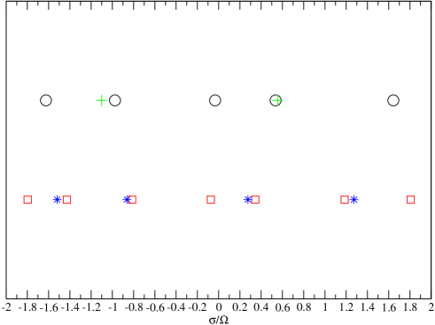
Figure 1: Positions of the eigenfrequencies calculated in the WKBJ approximation and the numerical results obtained by LF on the $\sigma/\Omega$ axis are plotted for the case $|m|=2$. The open circles and squares are obtained from the WKBJ approach and the pluses and stars give the results of the numerical computations of LF. The circles (pluses) correspond to modes having $l=l_{min}$ while the open squares (stars) correspond to modes with $l=l_{min}+1$.

In this section we compare the frequencies obtained from the approach described above with those obtained by a number of authors who have employed a variety numerical methods.

To obtain the values from the above analysis we use equation (66) for the eigenfrequencies, and, in the case of non zero $m$, add the expression for the correction to the frequency given by (109). We compare the results for polytropes with polytropic indices $n=1$, and $1.5$. The quantities $B_{n}$ entering (109) for these cases were obtained numerically with help of equation (100). We found $B_{1}\approx 14.4$ and $B_{3/2}\approx 5.97$. The range of allowed values of $k$ is found from equation (68). Additionally, we shall discard modes, which have $|\mu|$ close to $0$ or $1$ (see discussion below). We comment here that it follows from equation (109) that the frequency correction $\sigma^{m}_{1}$ becomes undefined for such values of $\mu.$

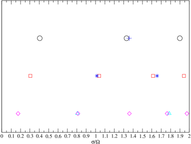
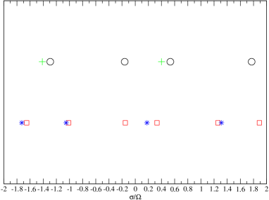
Figure 2: As for Fig. 1 but the left panel illustrates the case $m=0$ and the right hand side panel corresponds to $|m|=1.$. In the left panel we also show the locations of the WKBJ modes corresponding to $l=4$ (diamonds) and the locations of two eigenfrequencies calculated by Dintrans $\&$ Ouyed (2001) (triangles).

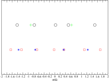
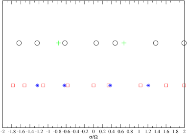
Figure 3: As for Fig. 1 but for the case of $|m|=3$ (left panel) and $|m|=4$ (right panel).

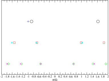
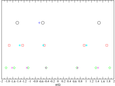
Figure 4: The result of comparison of the odd modes. Circles, squares and diamonds show positions of the WKBJ modes, corresponding to $l^{o}=0,1,2$, respectively. Pluses, stars and crosses give positions of frequencies numerically calculated by LF. The cases of $|m|=1$ (left panel) and $|m|=2$ (right panel) are shown.

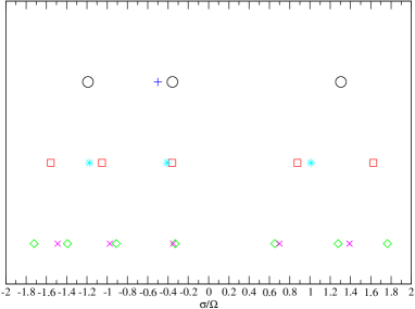
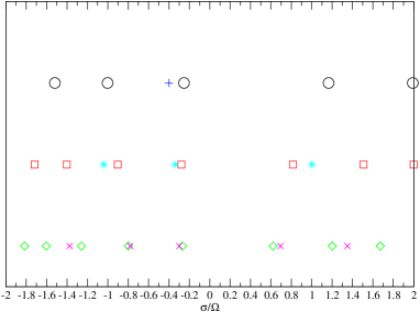
Figure 5: As for Figs. 4 but for the case of $|m|=3$ (left panel) and $|m|=4$ (right panel).

Most of the eigenvalues considered are for the model with $n=1$, which has been extensively discussed, (see eg. LF and Dintrans $\&$ Ouyed, 2001). The amount of attention paid to this model is due to the fact that it approximately reproduces the density distribution of a cold coreless Jupiter mass sufficiently below the planet’s surface. Some eigenvalues for planetary models (mostly the so-called ’global modes’ with $m=2$ and $l=1$) were calculated by IP. The properties of the global modes in this case are very similar to those of a polytrope with $n=1.$ Since the different numerical approaches essentially agree with each other for the case $n=1$ with non zero values of $m,$ we compare our results with the numerical values obtained by LF.

LF consider both even and odd modes and classify the mode order by an integer $l_{0}$, which is related to integer $p$ defined in equation (67) through $l_{0}=p+|m|-1$. Let us remind that when the even modes are considered $p=2l$, see equation (65), and for the odd modes $p$ is related to the integer $l^{o}$ classifying the odd modes as $p=2l^{o}+1$, see equation (126) of Appendix A. Using this definition, it is easy to see that LF give eigenfrequencies of modes having even symmetry with $l=l_{min}=1$ and $l=2$ for the case $|m|>0$ and $l=l_{min}=2$ and $l=3$ for the case $m=0.$ For the case of $m=1,$ we also considered the next order even modes with $l=4$ and compared eigenfrequencies with what was obtained by Dintrans $\&$ Ouyed (2001). We also compare the WKBJ odd modes for $m=1,2,3$ and $4$ with the results of LS. The integer $l^{o}$, in this case, takes the values $l^{o}=l^{o}_{min}=0,1$ and $2$. For the case $n=1.5$ the comparison of the WKBJ eigenfrequencies is made with the numerical results obtained by spectral methods in PI.

The results of the comparisons for $n=1$ are shown in Figs. 1- 5, where positions of the eigenfrequencies within the allowed range $-2<\sigma/\Omega<2$ are shown. The WKBJ eigenfrequencies, $\sigma$ are found from

$$\sigma=\sigma_{*}+\sigma_{1}^{m},$$ (113)

where $\sigma_{*}=2\mu$, and $\mu$, $\sigma^{m}_{1}$ are given by equations (66), (109), respectively. In our analytical investigation we assumed that the quantity $\mu$, and, accordingly, $\sigma_{*}$, is positive, but allowed the sign of the azimuthal number $m$ to be either positive or negative. For the purpose of this section it is convenient to take a different but equivalent point of view and assume that the sign of $m$ is fixed: $m>1$ and allow the quantities $\sigma_{*}$ to have either sign. The positive and negative signs correspond to prograde and retrograde mode propagation with respect to direction of rotation of the planet, respectively.

Let us first discuss the result of comparison of the even modes, which is presented in Figs. 1-3.

In Fig. 1 illustrates the case with $m=2.$ This is the most important value when one considers the problem of dynamical tides excited by a perturbing companion. The WKBJ eigenfrequencies are shown as open circles for $l=1$ and squares for $l=2$, respectively. The corresponding numerical values are indicated by crosses and stars. As seen in Fig. 1, the numerical and analytical values show quite good agreement with each other. This agreement is good even for the modes with the smallest possible value of $l=1,$ which have a global distribution of perturbed quantities over the volume of the star and therefore might not be expected to be in any kind of agreement with the results of a WKBJ theory. This might be explained by the rather large value of the parameter $\lambda$ for these modes, being equal to $5.5.$ From the discussion above, its inverse $\lambda^{-1}\approx 0.18$ is assumed to be a small parameter in our WKBJ expansions. There are, however, three unidentified modes for the case $l=1$ as well as for $l=2$. These modes have frequencies concentrating near the borders of the allowed frequency range with $\sigma\approx\pm 2$ as well as in the region close to $\sigma=0.$ It is possible that although these correspond to global modes for the incompressible $(n=0)$ model, these do not retain their character when $n$ is increased to $1$ and beyond through a strong coupling to short wavelength modes nearby in eigenfrequency (see discussion in section 2.5). Discarding these modes, hereafter referred to as unidentified modes, the relative difference between the analytical and numerical results is of order of or smaller than $10$ per cent.

In Fig. 2 we illustrate the case with $m=0$ in the left panel and the case with $m=1$ in the right panel. For $m=0$ the eigenfrequency distribution is symmetric with respect to the reflection $\sigma\rightarrow-\sigma$, and, therefore, only positive values of $\sigma$ are shown. As for the previous case, when $m=0$ the agreement between the WKBJ values classified as ’physical’ and the results of the numerical study is quite good, even when the ’global’ mode with $\sigma\approx 1.3$ is considered, the relative difference being of the order of $3$ per cent for this mode . Again, this may be accounted for by the relatively large value of $\lambda=5.5$ for $m=0$ and $l_{min}=2.$ Additionally, on this plot we show the results of a calculation by Dintrans $\&$ Ouyed (2001). They calculated five modes for $m=0.$ Three of them have locations nearly the same as those obtained by LF. They are, therefore, not shown in the plot. As seen from the plot, the other two modes may be identified with with the analytical modes having $l=4$. Note that the agreement gets better with increasing WKBJ order $,l,$ as expected.

When $|m|=1$ the agreement is similar to the case with $|m|=2$ apart from the mode with $l=2$ and $k=2,$ where the WKBJ value $\sigma\approx 0.33$ is approximately twice as small as the numerical one. The reason for this disagreement is unclear to us. Note, however, that there seems to be a disagreement between numerical methods in this case. Only one of the modes with $l=2$ and $|m|=1$ obtained by LF can be reliably identified with an eigenfrequency given by Dintrans $\&$ Ouyed (2001). However, the ’global’ modes with $|m|=1$ and $l=1$ as well as all LF modes obtained for the case $m=0$ have their counterparts in the results of Dintrans $\&$ Ouyed 2001.

In Fig. 3 we show the cases of relatively large values of $|m|=3$ ( left panel) and $|m|=4$ (right panel). The agreement gets worse with increasing $|m|$, and in the case of the ’global’ mode with $|m|=4$, $l=1$ and the numerical value $\sigma/\Omega\approx 0.6,$ the disagreement is of the order of $30$ per cent. This may be explained by the fact that in our theoretical scheme the value of $|m|$ is assumed to be much smaller than the value of $\lambda$. However, for the mode with the largest disagreement the ratio $|m|/\lambda\approx 0.53$ is not very small.

In Figs. 4 and 5 the comparison of the odd modes is made. The results are similar to the previous case. Apart from the presence of unidentified WKBJ modes, all numerically obtained frequencies have well identified WKBJ counterparts. The agreement is getting better with increase of the WKBJ order $l^{o}$ and is getting worse with increase of the azimuthal number $m$. Note a rather good agreement between the ’global’ WKBJ and numerical modes corresponding to $l^{o}=0$. In fact, as was shown by PP (see also Papaloizou $\&$ Pringle 1977), eigenfrequencies and eigenfunctions of these modes can be calculated analytically giving very simple results

$$\sigma=-{2m\Omega\over m+1},\quad W=z\varpi^{m}.$$ (114)

Note that neither eigenfrequencies nor eigenfunctions depend on the planet’s density distribution in this case.

In summary, we point out that agreement between the numerical and WKBJ frequencies is unexpectedly good taking into account the fact that the WKBJ theory should not, strictly speaking, be applied to modes with such small values of $\lambda.$ Apart from the existence of the unidentified modes in the WKBJ scheme and the two ’physical’ even modes and the global odd mode corresponding to $m=4$ with the rather large disagreements alluded to above the agreement between analytical and numerical results is of the order of or smaller than $15-20$ per cent for all the remaining identified $27$ even and $35$ odd modes. As we shall see below, good agreement is also found when the spatial distribution of the modes is compared.

4.1 Properties of eigenfunctions

In order to calculate distributions of the quantity $W$ over the volume of the planet we use equation (49) in the bulk of the planet and equation (71-77) close to the surface and smoothly interpolate between the two regions. Since the function $\eta[x]$ defined in section 3.7 is inconvenient for a numerical implementation we consider instead of it a function, which is zero in the regions $[0,1-x_{*}]$ and $[x_{*},1]$ and represented as a ratio of two polynomials of $x$ in the intermediate region, which are chosen in such a way to ensure that several first derivatives are equal to zero in both points $x=1-x_{*}$ and $x=x_{*}$.

Let us stress that for self-consistency we use the frequency $\sigma_{*}$ (or $\mu$) as given by equation (66) in those equations even when the frequency correction is non zero. As above, the numerical results for the $n=1.5$ polytrope are taken from PI. The WKBJ results for $n=1$ are compared with those obtained for a realistic model of a planet of one Jupiter mass. This model has a first order phase transition between metallic and molecular hydrogen, which has been discussed, eg., in IP.

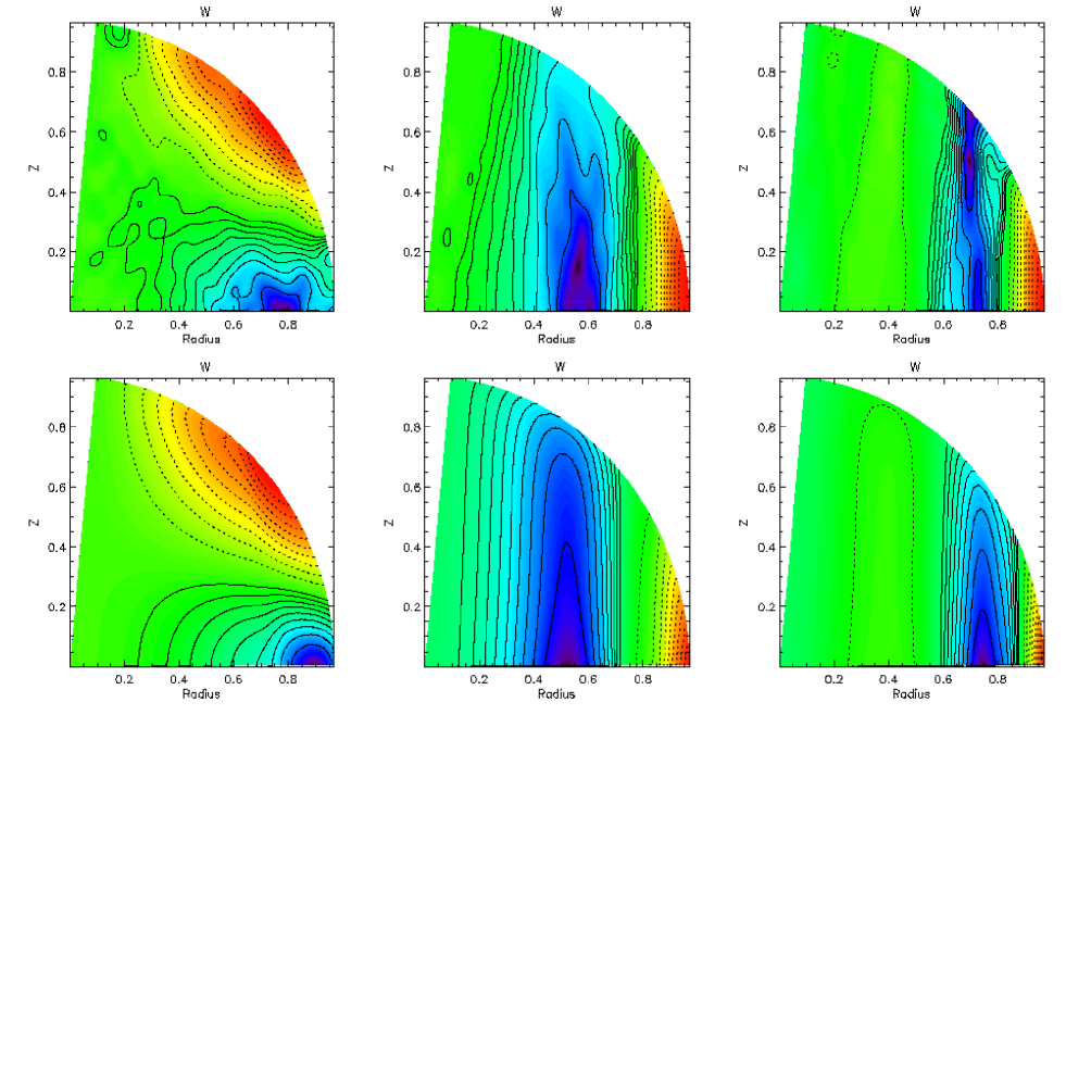
Figure 6: Distribution of $W$ over the surface of the star for the $n=1.5$ polytrope. The upper plots are obtained by numerical methods and the lower plots from the WKBJ theory. The values of eigenfrequencies are given in the text. From left to right the integers $l$ and $k$ determining the WKBJ eigenfrequencies are $l=1,k=0$, $l=1,k=1$ and $l=2,k=2$ respectively.

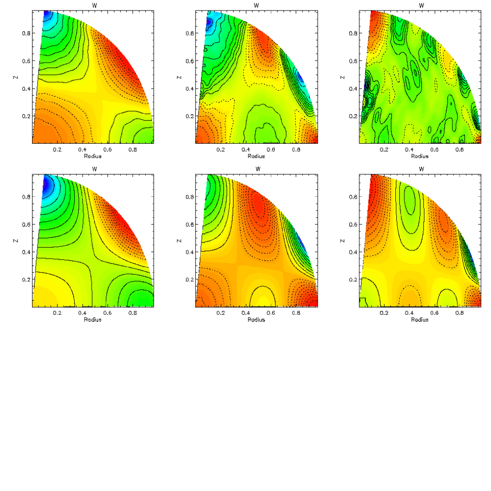
Figure 7: As for Fig. 6 but for $m=0.$ The upper plots represent numerical results for a planet with a realistic equation of state, the lower plots are calculated from the WKBJ theory assuming that $n=1.$ The eigenfrequencies are given in the text.

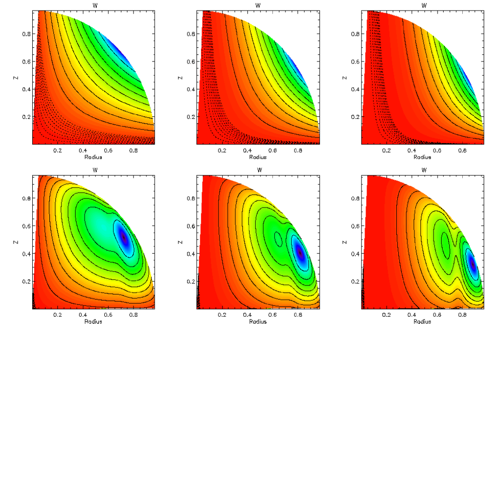
Figure 8: Distributions of $W$ for the global odd modes are shown. The azimuthal number $m=1,2,3$ from left to right. The upper plots represent the analytical results given by equation (114), the lower plots show the corresponding WKBJ counterparts.

A comparison of the different results is shown in Figs. 6 and 7. Note that in all cases shown in this section the same contour levels are used for the numerical and analytical data.

In Fig. 6 we show the distribution of $W$ over the planet’s volume for the $m=2$ modes and $n=1.5$. Numerical results are presented in the upper plots, which are taken from PI. These are for modes with $\sigma=-1.06$ ( upper left plot), $\sigma=0.67$ (upper middle plot) and $\sigma=0.67$ (upper right plot). The modes with $\sigma=-1.06$ and $\sigma=0.67$ are the so-called two main global modes, according to PI. They mainly determine transfer of energy and angular momentum through dynamic tides induced by a parabolic encounter. The respective WKBJ counterparts have the smallest possible WKBJ order $l=1$. The corresponding analytic eigenfrequencies are $\sigma=-0.99$ ($\sigma_{*}=-1.32$) and $\sigma=0.64$ ($\sigma_{*}=0.39$). The distribution shown on the upper right plot may be identified with a next order mode having $\sigma=0.435$ and $\sigma_{*}=0.29.$ One can see that there is a surprisingly good agreement between the analytical and numerical results. In particular, the retrograde mode represented on the left hand side plots has a ’spot’ in distribution at the angle $\approx\pi/4$ with respect to the rotational axis. This agrees with position of the critical latitude since $\arccos\mu=\arccos|\sigma_{*}/2|\approx 0.27\pi$. The distributions shown on the middle and right plots correspond to prograde modes. They have a well pronounced approximately vertical isolines. The main global mode may be distinguished from the mode corresponding to the next order by the number of nodes in the horizontal direction, this being one in the case of the global mode and two for the next order mode. We have checked that similar agreement exists between the WKBJ and numerical results corresponding to $n=1.$ Since the distributions are quite similar they are not shown here.

For $m=0$ we compare the WKBJ results with calculations done by a spectral method for a model of a planet of Jupiter size and mass in Fig. 7. As in the previous case the upper plots correspond to the numerical results. From left to right the numerical values of the eigenfrequencies are $1.35$ (the main global mode), $1.01$ and $0.79$. Their analytical counterparts have $l=2,k=1$, $\sigma=1.33$; $l=3,k=2$, $\sigma=1.03$ and $l=4,k=3$, $\sigma=0.83$ respectively. Note that a more pronounced disagreement in eigenfrequencies corresponding to the mode represented on the right hand side plot is mainly determined by the fact that this mode has a distribution concentrated near the surface of the planet, where the equation of state differs from that of a $n=1$ polytrope. One can see that again there is very good agreement between the results. This is especially good for the main global mode represented in the plots on the left hand side. The agreement gets somewhat worse moving from right to left. This may be explained by a number of factors such as inaccuracies of the numerical and analytical methods as well as the physical effects determined by changes of the equation of state in the outer layers of the planet and the presence of the phase transition. These factors mainly influence modes with a small spatial structure while the large scale main global mode is hardly affected by them.

Finally we consider the global odd modes and compare the analytic distributions given by equation (114) with the corresponding WKBJ distributions for $m=1,2$ and $3$ in Fig. 8. Although there is a disagreement in position of the spot close to the critical latitude, which is situated on the planet’s surface in the case of the exact analytic solutions and slightly interior to the surface of the planet in the case of the WKBJ distributions, there is a similarity in the distributions in the planet’s interior. This is quite surprising since in this case the analytic distributions do not depend on the planet’s structure at all while the WKBJ distributions are determined by the density distribution close to the planet’s surface.

5 Discussion

5.1 Overlap integrals

As we pointed out in the Introduction, integrals of the form

$$\hat{Q}_{k}={Q_{k}\over\sqrt{N}_{k}}\quad{\rm with}\quad Q_{k}=({\rho\over c_{s}^{2}}W_{k}|\Phi),$$ (115)

where $W_{k}$ corresponds to a particular eigenmode and $\Phi$ is some smooth function, appear in astrophysical applications of the theory developed in this paper. In particular, as was discussed in PI and IP, integrals of this type enter in expressions for the transfer of energy and angular momentum transferred during the periastron passage of a massive perturber. These apply to the case when the spectrum of normal modes is discrete and they involve integrals of form (115), where $\Phi=P_{2}^{m}r^{2}$ with $P_{2}^{m}$ being the associated Legendre function. Assuming that $W_{k}$ varies on a small spatial scale while the function $\Phi$ is smoothly varying such integrals may, in principal, be evaluated using our formalism with help of a theory of asymptotic evaluation of multidimensional integrals, see eg. Fedoryuk (1987), Wong (1989).

However, some important integrals of form (115) require an extension of our formalism, which can provide a smooth matching of the solution close to the surface to the WKBJ solution in the inner part of the planet that is valid at the next orders in inverse powers of $\lambda$. This is due to cancellations of leading terms in corresponding asymptotic series. Since this problem appears to be a rather generic one we would like to discuss it here in more detail for the important case when $\Phi=P^{2}_{2}r^{2}=3\varpi^{2}$. The overlap integral of this type determines excitation of the $m=2$ modes which are the most important for the tidal problem (eg. PI, IP and see also PIN). Explicitly, we have in this case

$$Q_{k}=3\int dV\left(\varpi^{2}{\rho\over c_{s}^{2}}W_{k}\right),$$ (116)

where $dV=dz\varpi d\varpi$. Note that this integral must converge to zero in the incompressible limit $n\rightarrow 0$ as in this case it is well known that inertial modes are not excited in the anelastic approximation. This fact, however, is not obvious for the integral written in the form (116) because close to the surface we have

$${\rho\over c_{s}^{2}}\approx nCx^{(n-1)},$$ (117)

with the constant $C$ converging to a nonzero value as $n\rightarrow 0.$ Therefore, as the eigenfunctions are regular, the integral $Q_{k}/n$ has a logarithmic divergence at the surface of the planet as $n\rightarrow 0.$ This raises the possibility that the overlap integral might converge to a nonzero value or behave pathologically as the incompressible limit is approached.

In order to show that, in fact, this is not so and $Q_{k}(n\rightarrow 0)\rightarrow 0$ in a smooth manner, let us consider some fiducial models having the property that the quantity

$$\omega_{0}^{2}=-\frac{c^{2}_{s}}{r\rho}\frac{d\rho}{dr}$$ (118)

is constant. For models in hydrostatic equilibrium under their own gravity, constancy of $\omega_{0}^{2}$ implies that ratio $M(r)/r^{3}$, where $M(r)$ is the mass interior to the radius $r,$ is constant. The model must accordingly be incompressible. Goodman $\&$ Lackner (2009) obtained a wider class of models in hydrostatic equilibrium under a fixed quadratic gravitational potential. Because the potential is fixed independently of the mass distribution and there are no constraints on the equation of state, such models may be constructed for an arbitrary density distribution.

Now let use consider the integral

$$Q_{fud}=3\int dV\left(\varpi^{2}{\rho\over c_{s}^{2}}\omega_{0}^{2}W_{k}\right).$$ (119)

For the fiducial models described above this is identical to the overlap integral (116) where we note that we may adopt natural units such that the constant $\omega_{0}^{2},$ which should be identified with the surface value of $GM(r)/r^{3}$ is equal to unity in that case. More generally the integrand in (119) can be transformed using equation of hydrostatic equilibrium (118) such that

$$Q_{fud}=-3\int dV\left({\varpi^{2}\over r}{d\rho\over dr}W_{k}\right)=-3\int dV\left(\varpi{\partial\rho\over\partial\varpi}W_{k}\right).$$ (120)

Now let us consider equation (11) for free normal modes in the anelastic approximation by setting $\sigma=\sigma_{k}$ and the right hand side of this equation to zero. Then we multiply it by $\varpi^{2}$, set $m=2$, and integrate over $dV$. After removing derivatives of $W_{k}$ by integrating by parts, assuming that the density vanishes at the surface boundary, it is easy to see that it follows from (11) that $Q_{fud}=0$ in the anelastic approximation provided $\sigma_{k}\neq 2\Omega.$ This means, in particular, that $m=2$ inertial waves cannot be excited in the Goodman $\&$ Lackner (2009) models in this approximation as was found by these authors when compressibility was fully taken into account (see PIN for additional discussion).

Using the fact that $Q_{fud}=0$ we may rewrite (116) for models under their own self-gravity quite generally, adopting natural units, as

$$Q_{k}=Q_{k}-Q_{fud}=3\int dV\varpi^{2}{\rho\over c_{s}^{2}}\left(1-\frac{M(r)}{r^{3}}\right)W_{k}.$$ (121)

Taking into account that the factor in the brackets is proportional to $x$ for small $x$, and, accordingly, in this limit the integrand is proportional to $nx^{n}$ we see that now the logarithmic divergence of $Q_{k}/n$ disappears and, therefore, it is clear from the representation (121) that the overlap integral indeed smoothly tends to zero in the limit $n\rightarrow 0$.

The theory of asymptotic evaluation of integrals of the form (121) tells that the values of such integrals are determined either by inner stationary points, where gradient of the WKBJ phase vanishes or contributions close to the surface or other parts of the integration domain, where the WKBJ approximation is not valid. From the expression of the $W_{k}$ in the WKBJ regime (49) it follows that there are no stationary points in the inner region of the planet. Considering the regions close to the surface it appears to be reasonable to assume that the leading contribution is determined by the region close to the critical latitude, where a ’hot spot’ is observed in distributions of $W_{k}$, see the previous section. In this region the quantities $\delta_{1}=x_{1}-\mu$ and $\delta_{2}=\mu-x_{2}$ are small. We can use them as new integration variables in (121) with help of (96), separate the contribution of this region to the integral by introduction of the functions $\eta[\delta_{1,2}]$ defined in section 3.7 in the integrand, and decompose the quantities in front of $W_{k}$ in powers of $\delta_{1,2}$ taking into account that $x\propto\delta_{1}\delta_{2}$ and $\varpi^{2}\approx(1-\mu^{2})$ in the leading order. Assuming that $W_{k}\approx\bar{W}(\delta_{1})\bar{W}(\delta_{2})$, where $\bar{W}(y)$ is given by equation (70), it is easy to see that the leading contribution to (115) is given by a symmetric combination of two integrals involving Bessel functions

$$Q_{k}\propto I_{1}(\delta_{1})I_{2}(\delta_{2})+I_{2}(\delta_{1})I_{1}(\delta_{2}),$$ (122)

where

$$I_{1}(y)=\int_{y=0}dy\eta[y]y^{n}J_{(n-1)/2}(\kappa y),\quad I_{2}(y)=\int_{y=0}dy\eta[y]y^{(n+1)}J_{(n-1)/2}(\kappa y),$$ (123)

where it is assumed that $\eta[y>y_{*}]=0$, $y_{*}$ lies within the range of integration and $1/\kappa\ll y_{*}\ll 1$. As was shown by Larichev (1973) the integral $I_{1}(y)=0$ for any particular form of the function $\eta[y]$. Thus, the leading order contribution to the overlap integral from the surface region close to the critical latitude is equal to zero. In principal, one can look for the next order terms. However, in this case our simple approach to the problem seems to be inadequate since eg. the assumption that $W_{k}$ can be represented as a product of two functions separately depending on the coordinates may be broken at this level, etc.. A more accurate approach is left for a future work. We note, however, that this cancellation means that the overlap integral should decay rapidly with increasing $\lambda,$ possibly being inversely proportional to a large power of $\lambda.$ This may qualitatively explain why a small number of relatively large scale modes are significantly excited by dynamic tides, see PI, IP and PIN.

5.2 Conclusions

In this paper we have developed a WKBJ approximation, together with a formal first order perturbation approach for calculating the normal modes of a uniformly rotating coreless planet under the assumption of a spherically symmetric structure. Matching of the general WKBJ form valid in the interior to separable solutions valid near the surface resulted in expressions for eigenfunctions that were valid at any location within the planet together with an expression for the associated eigenfrequencies given in section 3.5. Corrections as a result of density gradient terms neglected in the initial WKBJ approach were also obtained from formal first order perturbation theory.

The corrected WKBJ eigenfrequencies obtained using the WKBJ eigenfunctions were compared with results obtained numerically by several different authors and found to be in good agreement, away from the limits of the inertial mode spectrum where identifications could be made, even for modes with a global structure. We also compared the spatial forms of the eigenfunctions with those obtained using the spectral method described in IP finding similar good agreement.

This is consistent with the idea that these global modes can be identified and that first order perturbation theory works even though they are embedded in a dense spectrum.

In further support of this, the formal first order perturbation theory developed here is subsequently used to estimate corrections to the eigenfrequencies as a consequence of the anelastic approximation and is then compared with simulation results for a polytropic model with $n=1$ in PIN. These different approaches are found to be in agreement for small enough rotation frequencies and also indicates that, as implied by the simplified discussion in section 2.3 of this paper, that corrections as a result of the anelastic approximation are never very significant for the models adopted.

Our results show that the problem of finding eigenfrequencies and eigenvalues of inertial modes allows for an approximate analytical treatment, even in the case of modes having a large scale distribution of perturbed quantities.

Although we consider only the case of a polytropic planet, our formalism can be applied to a much wider context. Indeed, the approach developed here is mainly determined by the form of the density close to planet’s surface, where we assume that it is proportional to a power of distance from the surface. Thus, we expect that our main results remain unchanged for any density distribution, which is approximately power-law close to the surface. In particular, according to our results, all models of type having approximately the same behaviour of the density distribution close to the surface should have approximately the same eigenspectrum.

The formalism developed here can be extended for an approximate analytic evaluation of different quantities associated with inertial modes, such as overlap integrals characterising interaction of inertial waves with different physical fields, growth rates due to the CFS instability and decay rates due to various viscous interactions and non-linear mode-mode interaction. It may provide a basis for a perturbative analytic analysis of more complicated models, such as realistic models of star and planets flattened by rotation or models of relativistic stars.

As we discussed above, for a given value of WKBJ order, $l,$ some modes are identified with modes obtained numerically while others remain unidentified. Eigenfrequencies of the unidentified modes are always either situated close to the boundaries of the frequency range allowed for inertial modes, $\sigma=\pm 2\Omega$ or situated close to the origin $\sigma=0$. We believe that our theory is not applicable to these modes, and they develop a small scale contribution controlled by the closeness of the positions of their eigenfrequencies to $\sigma=0$ and $\pm 2\Omega,$ and thus effectively move to higher order than allowed for. Accordingly we de not consider these modes when comparing our results with results of direct numerical calculations of the excitation of inertial waves due to a tidal encounter reported in PIN.

Appendix A The eigenfrequencies of the ’odd’ WKBJ modes

In order to find the eigenfrequencies of modes odd with respect to reflection $z\rightarrow-z$ the phase $\phi_{2}$ should be chosen in such a way that the corresponding eigenfunctions are equal to zero at the planet equatorial plane, and, accordingly, $W(z=0)=W(y_{2}={\pi\over 2})=0$. From this condition and equation (42) we obtain

$$\phi_{2}=-\lambda{\pi\over 2}+{\pi\over 2}+\pi s,$$ (124)

where $s$ is an integer. Analogously to the case of even modes the phase $\phi_{1}$ is determined by equation (48) and the form of solution close to the surface is determined by equations (62) and (63). From these equations and equation (124) we get the compatibility conditions analogous to conditions (64)

$${\pi\over 4}n+\pi k_{1}=\lambda\arccos(\mu)-{\pi\over 2}|m|-{\pi\over 4}\quad{\rm and}\quad{\pi\over 4}n+\pi k_{2}=\lambda\left({\pi\over 2}-\arccos(\mu)\right)-{\pi\over 2}-\pi s,$$ (125)

and, solving (125) for $\lambda$ and $\mu$ we find that

$$\lambda=2l^{o}+|m|+n+{3\over 2},$$ (126)

where $l^{o}=k_{1}+k_{2}+s$, and that the expression for $\mu$ is given by equation (66), where (126) should be used. Comparing equations (65) and (126) we see that both even and odd modes can be described by the same expression for $\lambda$ provided that

$$\lambda=p+|m|+n+{1\over 2},$$ (127)

where $p=2l$ for the even modes and $p=2l^{o}+1$ for the odd ones, respectively.

Appendix B The oscillation spectrum of an incompressible fluid contained in a rotating spherical container in the WKBJ limit

In this appendix we show that the eigenvalues obtained from our WKBJ analysis agree with the corresponding values for an incompressible fluid contained in a rigid spherical container in the WKBJ limit.

B.1 Eigenvalues for the incompressible case in the WKBJ limit

It is well known that the spectrum of normal modes for an incompressible fluid in a rotating spherical container can be found analytically, ( see eg. Greenspan 1968, p. 64). The eigenfrequencies are determined from the equation

$$-mP^{|m|}_{s}(\mu)=(1-\mu^{2}){dP^{|m|}_{s}(\mu)\over d\mu},$$ (128)

where $P^{m}_{s}(\mu)$ is a Legendre function, $s$ is an integer, we recall that $\mu=\sigma/(2\Omega)$ and note that although it is inconsequential for the use of (B1), Greenspan’s definition of $m$ has the opposite sign to that used in this paper.

We determine the spectrum in the WKBJ limit from (128). In this limit $s$ is a large parameter. For our purposes it is important to retain all terms of order of $O({s^{-1}})$ and larger. We use the asymptotic form of Legendre functions in the limit of large $s$ in the form

$$P^{m}_{s}(\cos\phi)\propto{1\over\sqrt{\sin\phi}}\left\{\cos\left(\left(s+{1\over 2}\right)\phi-{\pi\over 4}+m{\pi\over 2}\right)+\left(m^{2}-{1\over 2}\right){\cos((s+{3\over 2})\phi+{\pi\over 4}+m{\pi\over 2})\over 2(s+{3\over 2})\sin\phi}\right\}.$$ (129)

Here we have used the well known properties of gamma functions to transform the asymptotic expression given in Gradshteyn $\&$ Ryzhik (2000) to the form (129).

We now substitute (129) into (128) after setting $\mu=\cos\phi$ in that equation. We then discard all terms $<O({s^{-1}}),$ thus obtaining

$$-m\cos\left(\left(s+{1\over 2}\right)\phi-{\phi\over 4}+|m|{\phi\over 2}\right)\approx s\sin\phi\sin\left(\left(s+{1\over 2}\right)\phi-{\pi\over 4}+|m|{\pi\over 2}\right)$$

$$+{1\over 2}\cos\left(\left(s-{1\over 2}\right)\phi-{\pi\over 4}+|m|{\pi\over 2}\right)+{1\over 2}(m^{2}-{1\over 4}\sin((s+{3\over 2})\phi+{\pi\over 4}+|m|{\pi\over 2}).$$ (130)

The quantity multiplying $s$ in the first term on the right hand side of (130) should be close to zero in order that this first term be of the same order as the other terms on the right hand side. This condition gives

$$\phi=\pi{j+{1/4}-{|m|/2}+\delta\over s+{1/2}},$$ (131)

where $j$ is an integer and $\delta$ is a small higher order correction. Setting it to zero we have

$$\mu_{0}=\cos\left(\pi{j+{1/4}-{|m|/2}\over s+{1/2}}\right).$$ (132)

This expression agrees with equation (66) when we consider the limit of incompressible fluid. To do this we set $n=0$ in (65) and (66), assume that $j-|m|=k$ and set

$$\lambda=s+{1\over 2}.$$ (133)

Comparing (133) with (65) we obtain

$$s=2l+|m|.$$ (134)

One can show that the requirement that $s-|m|$ is an even number determines eigenmodes for which $W$ has even symmetry with respect to the reflection $z\rightarrow-z$, see eg. Greenspan 1968, p. 65. Substituting (131) in (130) we get an expression for the correction $\delta$

$$\delta=-{m+{1\over 2}({3\over 4}+m^{2})\mu_{0}\over\lambda\sqrt{1-\mu_{0}^{2}}}.$$ (135)

Now we substitute (135) into (131) to obtain

$$\mu=\mu_{0}+{\mu_{0}\over 2\lambda^{2}}({3\over 4}+m^{2})+{m\over\lambda^{2}}.$$ (136)

The last term

$$\mu_{1}^{m}={m\over\lambda^{2}}$$ (137)

gives the leading order difference in eigenvalues belonging to eigenfunctions with values of $m$ of opposite sign. It is shown below that the expression (137) agrees with (109) provided that (109) is evaluated in the limit $n\rightarrow 0$.

B.2 The limit $n\rightarrow 0$ of the expression (109) for the frequency correction $\sigma_{1}^{m}$

If $n$ is directly set to zero, the integral (98) diverges at $y=0$. In order to find a limiting expression for (109) it is necessary to consider $n$ to be very small and take the limit $n\rightarrow 0$ in the final expression only after potentially divergent terms have been cancelled. Thus we assume that $n>0$ but very small and integrate (98) by parts to obtain

$$I_{n}={\pi\over 2}\int^{y_{*}}_{0}dyJ^{2}_{\nu}(y)={\pi\over 2}y_{*}J^{2}_{\nu}(y_{*})-\pi\int^{y_{*}}_{0}dyyJ_{\nu}{d\over dy}J_{\nu},$$ (138)

where $\nu=(n-1)/2$ and we remark that for $n>0$ $(yJ^{2}_{\nu}(y))\rightarrow 0$ when $y\rightarrow 0$. We use the well known relation

$$y{d\over dy}J_{\nu}(y)=\nu J_{\nu}-yJ_{\nu+1},$$ (139)

to eliminate the derivative of the Bessel function and obtain

$$nI_{n}=\pi[y_{*}J^{2}_{\nu}(y_{*})+\int_{0}^{y_{*}}dyyJ_{\nu}(y)J_{\nu+1}(y)].$$ (140)

It is easy to see that the expression on the right hand side does not diverge when $n\rightarrow 0$. However, the integral entering the right hand side of (140) diverges at large values of $y_{*}$. In order to deal with this divergence we use the asymptotic expression for the Bessel function, $J_{\nu}^{a}(y)$, valid at large values of its argument in the form,

$$J_{\nu}(y)\approx J^{a}_{\nu}(y)=\sqrt{{2\over\pi y}}\left\{\cos\left(y-\nu{\pi\over 2}-{\pi\over 4}\right)-{1\over 2y}{\Gamma(\nu+3/2)\over\Gamma(\nu-{1\over 2})}\sin\left(y-\nu{\pi\over 2}-{\pi\over 4}\right)\right\}.$$ (141)

From equation (141) it follows that the boundary term in (140) can be evaluated as

$$y_{*}J^{2}_{\nu}(y_{*})={1\over 2\pi}\left(1+\cos\left(2y_{*}-n{\pi\over 2}\right)\right)+O(y_{*}^{-1}).$$ (142)

Here we remark that because $y^{*}\sim\lambda x_{*},$ where $x_{*}$ is the dimensionless distance to the surface and $\lambda$ is large, $y^{*}$ may be large when $x_{*}$ is small corresponding to being close to the surface. Thus use of the asymptotic expansions of Bessel functions for large values of their arguments can be justified. In addition, setting $\nu=(n-1)/2$ and $\nu+1=n+1/2,$ (141) gives

$$J^{a}_{{n-1\over 2}}(y)J^{a}_{{n+1\over 2}}(y)\sim{1\over\pi y}\left(\sin\left(2y-n{\pi\over 2}\right)+{n\over 2y}\right),$$ (143)

and

$$I_{*}(y_{*})\equiv\int^{y_{*}}_{0}dyyJ^{a}_{{n-1\over 2}}(y)J^{a}_{{n+1\over 2}}(y)\sim-{1\over 2\pi}\cos\left(2y_{*}-n{\pi\over 2}\right)+{n\over 2\pi}\ln y_{*}.$$ (144)

Now, restoring complete precision, we can represent the integral entering (140) as

$$\int_{0}^{y_{*}}dyyJ_{\nu}(y)J_{\nu+1}(y)=I_{*}(y_{*})+C_{n},$$ (145)

where the quantity $C_{n}$ does not contain any divergences and can be evaluated in the limit $n\rightarrow 0$ and $y_{*}\rightarrow\infty$.

Setting $n=0$ in (144) and using the exact expressions for the Bessel functions given by

$$J_{-{1\over 2}}=\sqrt{{2\over\pi y}}\cos y,\quad J_{{1\over 2}}=\sqrt{{2\over\pi y}}\sin y,$$ (146)

we find

$$C_{0}=\int^{y_{*}}_{0}dyyJ_{-{1\over 2}}(y)J_{{1\over 2}}(y)+{1\over 2\pi}\cos 2y_{*}={1\over 2\pi}.$$ (147)

Now we use (147), (144) and (145) together with equations (142) and (140) to obtain in the limit of small $n$

$$I_{n}\approx{1\over n}+{1\over 2}\ln y_{*}.$$ (148)

Using this together with (98) and (100) we deduce that

$$B_{n}=e^{2/n}.$$ (149)

Substituting (149) in (109) and taking the limit $n\rightarrow 0$ we get

$$\sigma_{1}^{m}={2m\Omega\over\lambda^{2}},$$ (150)

where we use the fact that $\rho_{c}/D=1$ as $n\rightarrow 0$. Recalling that $\mu={\sigma/(2\Omega)}$ we see that (150) is equivalent to (137).

References

- (1) Aldridge, K. D., Lumb, L. I., 1987, Nature, 325, 421
- (2) Andersson, N., 1998, ApJ, 502, 708
- (3) Arras, P., Flanagan, E. E., Morsink, S. M., Schenk, A. K., Teukolsky, S. A., Wasserman, I., 2003, ApJ, 591, 1129
- (4) Bryan, G. H., 1889, RSPTA, 180, 187
- (5) Chandrasekhar, S., 1939 An Introduction to the Study of Stellar Structure New York: Dover
- (6) Chandrasekhar, S., 1970, Phys. Rev. Lett., 24, 611
- (7) Dintrans, B., Ouyed, R., 2001, AA, 375, L47
- (8) Fokin, M. V., 1994, Sib. Adv. in Math., 4, N1, 18
- (9) Fokin, M. V., 1994, Sib. Adv. in Math., 4, N2, 16
- (10) Fedoryuk, M. V., 1987 Asymptotics: Integrals and Series (in Russian), Nauka, Moscow
- (11) Friedman, J. L., Morsink, S. M., 1998, ApJ, 502, 714
- (12) Friedman, J. L., Schutz, B. F., 1978, ApJ, 222, 281
- (13) Goodman, J., Lackner, G., 2009, ApJ, 696, 2054
- (14) Gradshteyn I. S., Ryzhik I. M., 2000, Table of Integrals, Series and Products, Sixth Edition, Academic Press, San Diego, London
- (15) Greenspan, H. P., The Theory of Rotating Fluids, 1968, Cambridge University Press
- (16) Ivanov, P. B., Papaloizou, J. C. B., 2004, MNRAS, 347, 437
- (17) Ivanov, P. B., Papaloizou, J. C. B., 2007, MNRAS, 376, 682 (IP)
- (18) Kokkotas, K. D., 2008, Rev. Mod. Astr., 20, 140
- (19) Landau, L. D., Lifshitz, E. M.,1977, Quantum Mechanics: Non-relativistic Theory, Third Edition, Elsevier Science Ltd, Oxford
- (20) Larichev, V. D., 1973, Journal of Computational Mathematics and Mathematical Physics (in Russian), 13, 1029
- (21) Lockitch, K. H., Friedman, J. L., 1999, ApJ, 521, 764 (LF)
- (22) Ogilvie, G. I., Lin, D. N. C., 2004, ApJ, 610, 477
- (23) Ogilvie, G. I., 2009, MNRAS, 396, 794
- (24) Papaloizou, J. C. B., Ivanov, P. B., 2005, MNRAS, 364, L66 (PI)
- (25) Papaloizou, J. C. B., Ivanov, P. B., 2009, MNRAS, submitted (PIN)
- (26) Papaloizou, J. C. B., Pringle, J. E., 1978, MNRAS, 182, 423
- (27) Papaloizou, J. C. B., Pringle, J. E., 1981, MNRAS, 195, 743 (PP)
- (28) Papaloizou, J. C. B., Pringle, J. E., 1982, MNRAS, 200, 49
- (29) Prudnikov, A. P., Brychkov, Yu. A., Marichev, O., 1986, Integrals and Series, Vol 1. Elementary Functions, New York: Gordon and Breach
- (30) Ralston, J., 1973, J. of Math. Anal. and Appl., 44, 366
- (31) Savonije, G.J., Papaloizou, J. C. B., 1997, MNRAS, 291, 633
- (32) Schaeffer, D. G., 1975, Studies in Applied Mathematics, 54, 269
- (33) Schenk, A. K., Arras, P., Flanagan, E. E., Teukolsky, S. A., Wasserman, I., 2002, Phys. Rev. D, 65, 024001
- (34) Stewartson, K., Rickard, J. A., 1969, J. Fluid Mech., 35, 759
- (35) Wong, R., 1989, Asymptotic Approximations of Integrals, Academic Press, San Diego
- (36) Wood, 1977, Proc. R. Soc. Lond. A., 358, 17
- (37) Wu, Y., 2005a, ApJ, 635, 674
- (38) Wu, Y., 2005b, ApJ, 635, 688