Dynamic tides in rotating objects: a numerical investigation of inertial waves in fully convective or barotropic stars and planets

Abstract

We perform direct numerical simulations of the tidal encounter of a rotating planet on a highly eccentric or parabolic orbit about a central star formulated as an initial value problem. This approach enables us to extend previous work of Ivanov & Papaloizou to consider planet models with solid cores and to avoid making an anelastic approximation.

We obtain a power spectrum of the tidal response of coreless models which enables global inertial modes to be identified. Their frequencies are found to be in good agreement with those obtained using either a WKBJ approach or the anelastic spectral approach adopted in previous work for small planet rotation rates. We also find that the dependence of the normal mode frequencies on the planet angular velocity in case of higher rotation rates can for the most part be understood by applying first order perturbation theory to the anelastic modes.

We calculate the energy and angular momentum exchanged as a result of the tidal encounter and for coreless models again find good agreement with results obtained using either the anelastic spectral method.

Models with a solid core showed evidence of the emission of shear layers at critical latitudes and possibly wave attractors after the encounter but the total energy exchanged during the encounter did not differ dramatically from the coreless case as long as the ratio of the core radius to the total radius was less than $50\%$, there being hardly any difference at all when this ratio was less than $25\%$ of the total radius. We give a physical and mathematical interpretation of this result.

Finally we are able to validate the use of the anelastic approximation for both the work presented here and our previous work which led to estimates of circularisation rates for planets in highly eccentric orbits.

1 Introduction

A significant number of extrasolar planets are found in close circular orbits around their central star while others are found in highly eccentric orbits. This is an indication that planet-planet scattering may have been important after formation and generated highly eccentric orbits that subsequently undergo circularisation with attendant tidal heating ( see Papaloizou & Terquem 2006 for a review and references therein). In order to investigate such a scenario the tidal interaction of a planet on a highly eccentric orbit with the central star has to be evaluated. This was considered in the non rotating case by Ivanov & Papaloizou (2004) and in the rotating coreless case using an anelastic approximation by Papaloizou & Ivanov (2005) and Ivanov & Papaloizou (2007) (hereafter referred to as PI and IP, respectively). The excitation of pulsations or normal modes of the planet is a key aspect of the tidal problem.

In this paper we extend our previous work by relaxing the anelastic approximation and considering planet models with solid cores. We investigate pulsations of a uniformly rotating fully convective or barotropic object by performing numerical simulations of tidal encounters considered as initial value problems. The formalism we adopt does not require an anelastic approximation to be made and so it enables both the response of the low frequency inertial modes of oscillation as well as the higher frequency $f$ and $p$ modes to be taken into account. As in our preceding studies we consider the pulsations to be excited in an object referred to hereafter as a ’planet’ as a consequence of moving on a parabolic orbit around a central object.

We calculate the energy and angular momentum exchanged after pericentre passage for a variety of pericentre distances and angular velocities of rotation of the planet. We also study the spectrum of normal modes that is excited and compare their properties with the analytic theory developed in our accompanying paper Ivanov & Papaloizou (2009) hereafter IPN and also results obtained using the anelastic spectral approach described in Ivanov & Papaloizou (2007) (hereafter referred to as IP) . This comparison finds good agreement between the different approaches, validating the use of the anelastic approximation for describing the inertial mode response.

We also consider the effects of introducing a solid core into the planet. Although we find evidence for the development of singular phenomena such as the emission of shear layers at critical latitudes and the formation of wave attractors (see Ogilvie & Lin 2004, Ogilvie 2009 and Rieutord & Valdettaro 2010 and references therein) and after the encounter, the energy exchanged is in general not changed by a very large amount and for a modest sized core hardly at all. We give both a physical and mathematical explanation for this result in appendix B.

The plan of the paper is as follows. In section 2 we review some definitions and basic equations relegating a description of the numerical scheme we use to solve initial value problems to appendix A. Note that no anelastic approximation is made here. In section 3 we go on to describe the results we obtained for the response of a simple model of a giant planet as a polytrope of index $n=1$ to tidal encounters. We present results for the total energy and angular momentum transferred to a planet without a solid core for the full range of rotation rates and a variety of encounter pericentre distances. We then go on to consider planet models with solid cores of radius $25\%$ and $50\%$ of the total radius illustrating evidence of the focusing of inertial waves, the emission of shear layers at critical latitudes and wave attractors, in these cases. The role of these phenomena has recently been emphasised by Ogilvie & Lin (2004) and Ogilvie (2009) for the situation where the planet is tidally forced while in a fixed circular orbit. However, in our case with the smaller core, the energy and angular momentum transferred hardy differs from what is found for the coreless case. In the larger core case the interaction is somewhat stronger with the energy transfer being about one order of magnitude larger for the model with a core.

In section 4 we obtain the normal mode frequencies for the coreless planet model by taking Fourier transforms of the time series provided by the post tidal interaction responses and locating peaks in the corresponding power spectra. The normal mode frequencies are compared with those obtained using the spectral method described in PI and also the WKBJ method described in IPN, both of which adopted an anelastic approximation. The spectra obtained from the simulations are seen to contain $p$ and $f$ modes in addition to the inertial modes. The frequency locations of the main global inertial modes are found to be in good agreement with those obtained by other methods for azimuthal mode numbers $m=0$ and $m=2.$

In section 4.1.1 we investigate the dependence of the simulation normal mode frequencies (or eigenfrequencies) on the planet rotation rate paying a special attention to the case of inertial waves. In the anelastic approximation it can be shown that eigenfrequencies of inertial modes are proportional to the planet’s rotation rate, $\Omega$, so it is natural to express their values in terms of it. This proportionality breaks down when the anelastic approximation is not used and the positions of the mode eigenfrequencies measured in units of $\Omega$ are shifted when it changes. We compare positions of the simulation normal mode frequencies with those obtained using the anelastic spectral method but with a correction obtained by applying the first order perturbation theory given in IPN. The agreement is very good apart for one case that is apparently affected by an avoided crossing.

For completeness we consider the tidal response of a coreless model of the type considered by Goodman & Lackner(2009) that is in hydrostatic equilibrium under a fixed quadratic gravitational potential in section 5. These authors pointed out that a simple analytic solution is available and shows that no inertial mode excitation is expected in this case. Our numerical results indicate that any residual inertial mode excitation occurring as a result of numerical effects is very small in this case as should be expected.

In section 6 we compare the total energy and angular momentum transferred to a coreless polytropic planet with the anelastic spectral results already given in IP. We conclude that these are in good agreement and therefore the anelastic approximation is a valid approximation. Thus we do not confirm the suggestion of Goodman & Lackner (2009) that these exchanges could be seriously overestimated as a consequence of its use. Finally in section 7 we discuss our results.

2 Basic definitions and equations

Here we adopt a spherical polar coordinate system $(r,\theta,\phi)$ and the associated spherical coordinate system with origin at the centre of mass of the planet.

We consider the response to a tidal perturbation with associated gravitational potential $\Psi_{ext}$ written as a Fourier series in terms of the azimuthal angle $\phi$ in the form

$$\Psi_{ext}={\cal R}e\sum_{m=0}^{\infty}\Psi_{ext,m}\exp({im\phi}).$$ (1)

Here ${\cal R}e$ denotes that the real part is to be taken and although the sum is in general over all $m,$ we consider only $m=0$ and $2$ here. Similar Fourier decompositions are used for the state variables of the planet. In the linear approximation each Fourier component responds individually to the corresponding component of the tidal potential.

The planet is characterised by its mass $M_{*}$, radius $R_{*}$ and the associated frequency

$$\Omega_{*}=\sqrt{GM_{*}\over R_{*}^{3}},$$ (2)

where $G$ is the gravity constant. The associated energy and angular momentum scales are $E_{*}=GM_{*}^{2}/R_{*}$ and $L_{*}=M_{*}\sqrt{GM_{*}R_{*}}$ respectively. For definiteness, we consider below a planet having approximately Jovian values of mass and radius: $M_{*}$=$2\times 10^{30}g$ and $R_{*}=7\times 10^{9}cm$. Accordingly, it is assumed that $E_{*}\approx 3.81\times 10^{43}$, $L_{*}\approx 6\times 10^{46}$ and $\Omega_{*}\approx 6.23\times 10^{-4}$ in $cgs$ units. Note, however, that our results, given in dimensional form, may be scaled to other values of $M_{*}$ and $R_{*}$ when expressed in the natural units introduced above.

Following our previous work (Papaloizou $\&$ Ivanov 2005, hereafter PI, Ivanov $\&$ Papaloizou 2007, hereafter IP) we assume in this paper that the planet moves on a highly eccentric (formally, parabolic) orbit around a source of gravity of mass $M$. In the parabolic limit the orbit may be characterised by its pericentre distance, $R_{p}$. The simulations carried out in this paper started with the perturbing mass at a distance eight times the pericentre distance. Tidal forces being proportional to the inverse cube of the distance are negligible beyond this point (see eg. Faber et al 2005). For fixed masses, as an alternative to the pericentre distance, in this paper we define an encounter through the parameter

$$\eta=\sqrt{M_{*}R_{p}^{3}/(MR_{*}^{3})},$$ (3)

first introduced by Press $\&$ Teukolsky 1977, hereafter PT. Note that this expression for $\eta$ is strictly speaking valid only when $M_{*}\ll M$. A more general expression is given in equation (26) of appendix A.

2.1 Perturbed equations of motion

We assume that the planet is rotating with uniform angular velocity ${\Omega}$ directed perpendicular to the orbital plane. The hydrodynamic equations for the perturbed quantities take the simplest form in the rotating frame which we use later on.

Since the planet is fully convective, the entropy per unit of mass of the planetary gas remains approximately the same over the volume of the planet, and the pressure $P$ can be considered as a function of density $\rho$ only, $P=P(\rho)$. The perturbations of the planet may be considered as adiabatic, and therefore the same functional dependence $P=P(\rho)$ holds during perturbation as well. This condition is often referred to as the barotropic condition. In the barotropic approximation the linearised Euler equations take the form (see PI)

$$\frac{\partial{\bf v}}{\partial t}+2{\mbox{\boldmath${\Omega}$}}\times{\bf v}=-\nabla W+\frac{{\bf f}_{\nu}}{\rho},$$ (4)

where

$$W=c_{s}^{2}\rho^{{}^{\prime}}/\rho+\Psi_{ext},$$ (5)

${\bf v}=(v_{r},v_{\theta},v_{\phi})$ is the Eulerian velocity perturbation, $\rho^{{}^{\prime}}$ is the Eulerian density perturbation, $c_{s}=\sqrt{dP/d\rho}$ is the adiabatic sound speed, ${\bf f}_{\nu}$ is the viscous or diffusive force pr unit volume and as indicated above $\Psi_{ext}$ is the external forcing tidal potential. The velocity perturbation ${\bf v}$ is related to ${\mbox{\boldmath${\xi}$}}=(\xi_{r},\xi_{\theta},\xi_{\phi}),$ the Lagrangian displacement vector, through

$$\frac{\partial{\mbox{\boldmath${\xi}$}}}{\partial t}={\bf v}.$$ (6)

The linearised continuity equation gives

$$P^{\prime}=\rho^{{}^{\prime}}c^{2}_{s}=-c^{2}_{s}\nabla\cdot(\rho{\mbox{\boldmath${\xi}$}}),$$ (7)

where $P^{\prime}$ is the Eulerian pressure perturbation. Note that the centrifugal term is absent in equation $(\ref{eq p3})$ being formally incorporated into the potential governing the static equilibrium of the unperturbed star and there is no unperturbed motion in the rotating frame.

As in our previous work (eg. Papaloizou $\&$ Pringle 1981, PI, IP) we shall neglect centrifugal distortion of the basic equilibrium which will enable us to adopt a spherically symmetric unperturbed model and density distribution. We additionally simplify matters by adopting the Cowling approximation which neglects perturbations to the planet gravitational potential, being equivalent to regarding the planet as moving in a fixed specified spherical potential. Although we shall adopt a standard polytrope with $n=1$ as the basic unperturbed model which is not very centrally condensed, the main focus is on the low frequency inertial modes for which self-gravity is not expected to play a very important role. This is especially the case for small scale modes and waves of the type that arise when a solid core is considered. The Cowling approximation should also be valid when estimating the effects of compressibility on these kinds of disturbances.

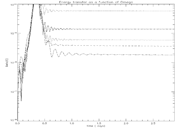
Figure 1: The energy measured in the rotating frame transferred to the planet as a function of time due to the $m=2$ tide is plotted for different angular velocities for an encounter with $\eta=4.$ The curves from the uppermost to lowermost at large times are for the non rotating case, $\Omega/\Omega_{*}=0.16,$ $\Omega/\Omega_{*}=0.36$ ( the curve obtained with twice the numerical resolution 400*400 is superposed and can barely be distinguished), $\Omega/\Omega_{*}=0.51$, $\Omega/\Omega_{*}=0.8$ and $\Omega/\Omega_{*}=1.12$ respectively (the latter case was considered for the purposes of illustrating trends). In this and other similar Figures below the time unit is days and the energy is expressed in units of the natural energy scale of the planet $E_{*}$.

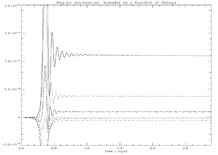
Figure 2: The angular momentum transferred to the planet induced by the $m=2$ tides is plotted as a function of time for different angular velocities for an encounter with $\eta=4.$ The curves from the lowermost to uppermost at large time are for $\Omega/\Omega_{*}=1.12,$ $\Omega/\Omega_{*}=0.8$, $\Omega/\Omega_{*}=0.51$, $\Omega/\Omega_{*}=0.36$ (curve for $400\times 400$ resolution superposed), $\Omega/\Omega_{*}=0.16$ and $\Omega=0$ respectively. In this and other similar Figures below the time unit is days and the angular momentum is expressed in units of the angular momentum scale of the planet $L_{*}$.

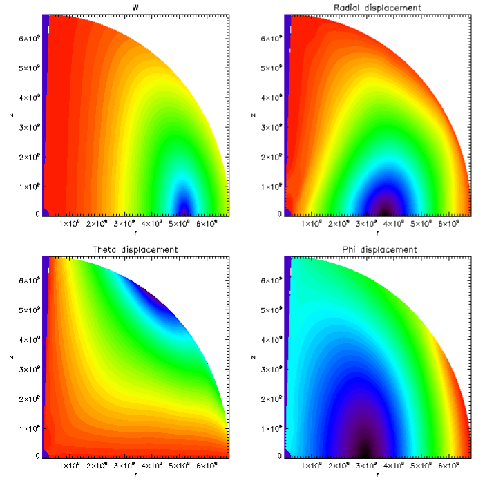
Figure 3: Contour plots for the real parts of the $m=2$ Fourier components of $W$ (upper left panel), $\xi_{r}$ (upper right panel), $\xi_{\theta}$(lower right panel) and $\xi_{\phi}$ (lower right panel) after $t=2.523days$ for the model with $\eta=4$ and $\Omega/\Omega_{*}=0.36.$ In this and other similar Figures, lengths are expressed in $cgs$ units. For reference $R_{*}=7\times 10^{9}.$

Provided that the expressions for the density, sound speed are specified for some unperturbed model of the planet as well as the form of the diffusive forces (see below) the set of equations $(\ref{eq p3}-\ref{eq p6})$ is complete. Details of its numerical solution are given in appendix A.

2.2 Addition of diffusive effects

Although problems of the type considered here are linear, because the spectrum is in a general sense singular, arbitrarily small scales can develop over time. It is important to note that such behaviour has a physical basis and does not arise from pure numerical artifacts.

For example the boundaries of the simulations we perform consist of the polar axis, the equatorial plane and the surface of the planet. Because of the coordinate singularity at $\theta=0,$ the polar axis is replaced by the cone $\theta=\theta_{n_{th}},$ see below, the latter angle being small. The angle between this cone and the equatorial plane is accordingly slightly less than a right angle. As shown by Ralston (1973), inertial waves with an appropriate frequency can undergo a sequence of alternating reflections at these boundaries, resulting in wave action accumulating in the corner, where the boundaries intersect. Hence a reflectosingularity is produced implying that such frequencies are in the continuous rather than point spectrum. Note that even small perturbations to boundaries can introduce effects of this type.

In order to avoid numerical problems arising from such phenomena we incorporate a diffusivity in the simulations which is adequate to effectively eliminate such artifacts in models with no specified central cores.

We added simple diffusive forces per unit volume in spherical coordinates of the form

$${\bf f}_{\nu}=\frac{\partial}{\partial r}\left(\rho\nu\frac{\partial{\bf v}}{\partial r}\right)+\frac{1}{r^{2}}\frac{\partial}{\partial\mu}\left(\rho\nu\sin\theta\frac{\partial{\bf v}}{\partial\mu}\right),$$ (8)

where the diffusion coefficient or effective kinematic viscosity $\nu=\nu_{0}\sqrt{GM_{*}R_{*}}$ was taken to be a constant. For the simulations reported here with coreless models and a grid resolution of $200\times 200$ (for more information about the numerical grid see appendix A), we adopted $\nu_{0}=9.36\times 10^{-6}$, and for these models with a grid resolution of $400\times 400$ we adopted $\nu_{0}=4.68\times 10^{-6}.$ For models with core radius $0.25R_{*}$ we adopted $\nu_{0}=4.57\times 10^{-5}$ at a grid resolution of $200\times 200$ and $\nu_{0}=2.28\times 10^{-5}$ at a grid resolution of $400\times 400.$ Finally, for models with core radius $0.5$ we adopted $\nu_{0}=1.7\times 10^{-5}$ at a grid resolution of $400\times 400$ and $\nu_{0}=8.5\times 10^{-6}$ at a grid resolution of $800\times 800.$ With these choices the diffusivity decreases as the resolution increases. We remark that energy and angular momentum transfers measured by evaluating the canonical energy and angular momentum (see appendix A) just after the encounter are robust to changes in numerical resolution and diffusivity as they should be (see below).

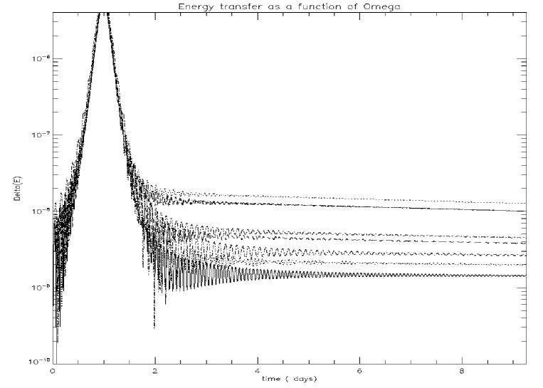
Figure 4: The energy transferred to the planet as a function of time due $m=2$ tide is plotted for different angular velocities for an encounter with $\eta=8\sqrt{2}.$ The curves from the uppermost to lowermost at large time are for $\Omega/\Omega_{*}=0.36,$ $\Omega/\Omega_{*}=0.27$ (the curve obtained for $\Omega/\Omega_{*}=0.45$ overlaps), $\Omega/\Omega_{*}=0.6$, $\Omega/\Omega_{*}=0.17,$ $\Omega/\Omega_{*}=0.8,$ $\Omega/\Omega_{*}=0.1$ and $\Omega/\Omega_{*}=0$, respectively.

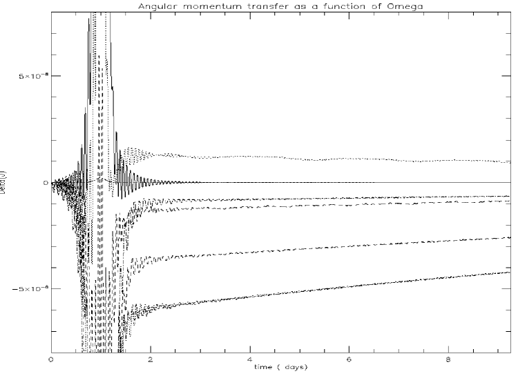
Figure 5: The angular momentum transferred to the planet is plotted as a function of time for different angular velocities for an encounter with $\eta=8\sqrt{2}.$ The curves from the uppermost to lowermost at large time are for $\Omega/\Omega_{*}=0.1,$ $\Omega=0,$ $\Omega/\Omega_{*}=0.8,$ $\Omega/\Omega_{*}=0.6,$ $\Omega/\Omega_{*}=0.17,$ $\Omega/\Omega_{*}=0.45$ and $\Omega/\Omega_{*}=0.27$ ( the curve obtained for $\Omega/\Omega_{*}=0.36$ overlaps), respectively.

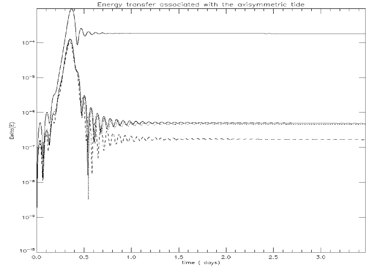
Figure 6: The energy transferred to the planet as a function of time due to the axisymmetric tide $(m=0)$ is plotted for different angular velocities for an encounter with $\eta=4.$ The lowermost curve at large times corresponds to $\Omega/\Omega_{*}=0.8,$ the curve immediately above this to $\Omega/\Omega_{*}=0.36$ and curve immediately above that , which is almost coincident, is for the non rotating case. For purposes of comparison the uppermost curve is for the non rotating case with the $m=2$ component of the tidal potential.

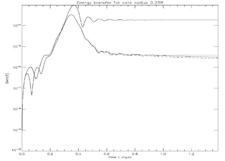
Figure 7: The energy transferred to the planet as a function of time due to the $m=2$ tide is plotted for a model with a solid core of radius $0.25R_{*}.$ The encounter is for $\eta=4$ and $\Omega/\Omega_{*}=0.8.$ The curves from the lowermost to uppermost at large time are for a resolution of $200\times 200,$ a resolution of $400*400,$ for comparison a model with no core and a model with no core and no rotation.

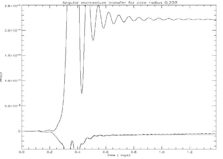
Figure 8: The angular momentum transferred to the planet as a function of time due to the $m=2$ tide is plotted for a model with a solid core of radius $0.25R_{*}.$ The encounter is for $\eta=4$ and $\Omega/\Omega_{*}=0.8.$ The curves from the lowermost to uppermost at large time are for a resolution of $800\times 800,$ a resolution of $400*400,$ for comparison a model with no core and a model with no core and no rotation.

3 A general description of numerical results

3.1 The energy and angular momentum transfer for a close encounter

We here give results for the energy and angular momentum transfer as a result of a tidal encounter at fixed pericentre distance for different angular velocities. We have considered a range of $\Omega/\Omega_{*}$, where $\Omega_{*}$ is defined in equation (2), up to $1.12$ even though we have neglected centrifugal terms in the model. This is done in order to more fully explore and gain understanding of the functional dependence of the response on its defining parameters. The introduction of centrifugal terms would not change the essential response problem although deviations of the form of the effective surface boundary may play some role (see eg. discussion in section 2.2 above).

A first set of runs was carried out for $\eta=4$ taking into account the $m=2$ component of the tidal forcing. The contribution from this has found to dominate that of the $m=0$ component (see below). In all of these and other similar cases with no interior solid core, after the encounter the canonical energy and angular momentum attain either expected constant values or values that slowly decay on account of the imposed numerical diffusion. We have considered resolutions of $200\times 200,$ $400\times 400$ and for models with solid cores $800\times 800.$ As illustrated below the energy and angular momentum transferred between central object and planet is measured just after the encounter. This measures the physical exchange and is numerically converged.

The energy transferred to the planet as a function of time due to the $m=2$ tide is plotted for different angular velocities for an encounter with $\eta=4$ in Figure 1. Results are given for the non rotating case, $\Omega/\Omega_{*}=0.16,0.36,0.51,0.8$ and $\Omega/\Omega_{*}=1.12$, respectively. The angular momentum transferred to the planet as a function of time for the cases illustrated in Figure 1 are plotted in Figure 2. The energy transferred is seen to decrease monotonically with angular velocity by about a factor of thirty as $\Omega$ varies between zero and the maximum value considered. The energy transferred is expected to decrease as the star is spun up from zero (Ivanov & Papaloizou 2004) but may increase again at large values of $\eta$ (see PI, IP and below).

The angular momentum transferred to the planet has a maximum absolute value for the non rotating model and decreases with increasing angular velocity, becoming zero when $\Omega/\Omega_{*}=0.51.$ For larger values of $\Omega$ angular momentum is transferred from the planet to the star. Such a sign change is indeed expected when $\Omega$ is comparable to the angular velocity at pericentre, see PI and IP. We remark that the simulations for $\Omega/\Omega_{*}=0.36$ were done at resolutions of $200\times 200$ and $400\times 400$ and are illustrated in Figures 1 and 2. The results of these are indistinguishable.

The form of the planet response in these cases is found to be global. To illustrate this, contour plots for the real parts of the $m=2$ Fourier components of $W,$ $\xi_{r},$ $\xi_{\theta}$ and $\xi_{\phi}$ (lower right panel) after $t=2.523days,$ well after the encounter is complete, for the simulation with $\Omega/\Omega_{*}=0.36$ are shown in Figure 3 These have global form that is typically found at any time. As expected, there is no evidence of evolution to small scale structures indicative of the emission of shear layers at critical latitudes and wave attractors (eg. Ogilvie & Lin 2006, Rieutord & Valdettaro 2010) in these cases. The global form is indicated both by the accurate conservation of canonical energy and the accurate conservation angular momentum even though some numerical diffusion was present and also that the energy and angular momentum transferred is in good agreement with values obtained using a basis function approach developed in our previous papers PI and IP with a relatively small number $15\times 15$ of trial functions, see the next section.

3.2 The energy and angular momentum exchanged for a more distant encounter

We now consider simulations of the above form but with a larger value of $\eta=8\sqrt{2}.$ In addition to the non rotating case, the angular velocities considered were $\Omega/\Omega_{*}=0.36,0.27,$ $0.45,0.6,$ $0.17,0.8$ and $0.1.$ The energy transferred to the planet as a function of time is illustrated in Figure 4, and the angular momentum transferred to the planet is illustrated in Figure 5 . In this case the energy transferred initially increases with angular velocity but attains a maximum value before decreasing again. The reason for this behaviour is that the $f$ mode is ineffective at this value of $\eta$ leading to a weak interaction for the non rotating model. However, once the star is spun up, the interaction can strengthen through the inertial mode response. In this case the maximum transfer occurs for $\Omega/\Omega_{*}\sim 0.36.$ Similarly the angular momentum transfer is very small for the non rotating model It increases to a maximum for $\Omega/\Omega_{*}=0.1$ and then passes through zero at $\Omega/\Omega_{*}\sim 0.13.$ For larger angular velocities angular momentum is transferred from the planet to the star, this transfer being largest in magnitude when $\Omega/\Omega_{*}\sim 0.32$ beyond which it decreases in magnitude. The sign change again occurs at a value of the angular velocity comparable to that at pericentre passage and the planet response remains global.

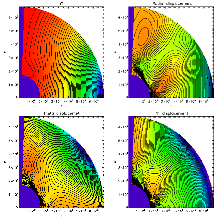
Figure 9: As in Figure 3 but for a model with core radius of $0.25R_{*}$ and $\Omega/\Omega_{*}=0.8$ after $t=0.408days.$

Figure 10: As in Figure 9 but at $t=0.776days$ and with contour line plots in order to illustrate the inertial wave propagation pattern

3.3 The axisymmetric case $m=0$ for $\eta=4$

In order to evaluate the effectiveness of the $m=0$ tide we carried out simulations using the $m=0$ component of the tidal potential for $\eta=4.$ The energy transferred to the planet as a function of time is plotted for $\Omega/\Omega_{*}=0.8,0.36$ and the non rotating case in Figure 6. The non rotating case for $m=2$ is also shown. The energy transfer for $m=0$ is always found to be an order of magnitude or more smaller than the corresponding $m=2$ contribution. Therefore this can be neglected.

3.4 Planet models with a solid core

3.4.1 A planet with core radius equal to $0.25R_{*}$

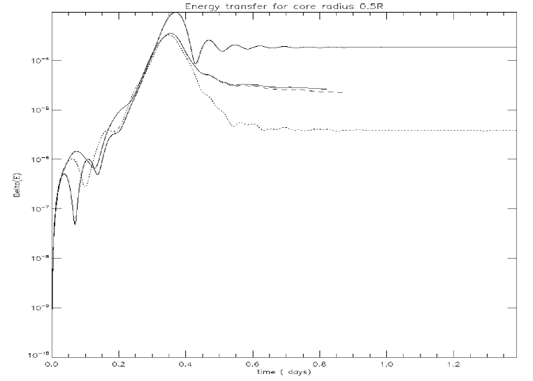
Figure 11: The energy transferred to the planet as a function of time due to the $m=2$ tide is plotted for a model with a solid core of radius $0.5R_{*}$. The encounter is for $\eta=4$ and $\Omega/\Omega_{*}=0.8.$ The curves from the lowermost to uppermost at large time are for a comparison model with no core, for a resolution of $400\times 400,$ for a resolution of $800*800,$ for further comparison a model with no core and no rotation.

We now go on to consider planet models with a solid core. In these cases the long term behaviour differs from the coreless models owing to the development of wave patterns related to critical latitude phenomena and wave attractors (eg. Ogilvie & Lin 2006, Ogilvie 2009 and references therein) that correspond to the development of increasing concentrations of wave energy along closed characteristic paths. However, it is important to note that our calculations are not for fixed frequency forcing, which is the situation considered for the discussion of critical latitude phenomena and wave attractors. Here we are concerned with a combination of different frequencies that should lead to a broader pattern. However, we still might expect that singular behaviour develops asymptotically for large time, in the non diffusive case. In the diffusive case this would be limited but energy dissipation would occur at an enhanced rate as compared to the non singular coreless models. This feature is observed in our simulations.

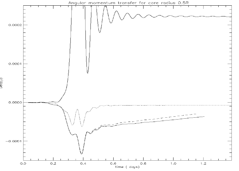
Figure 12: The angular momentum transferred to the planet as a function of time due to the $m=2$ tide is plotted for a model with a solid core of radius $0.5R_{*}.$ The encounter is for $\eta=4$ and $\Omega/\Omega_{*}=0.8.$ The curves from the lowermost to uppermost at large time are for a resolution of $800\times 800,$ for a resolution of $400*400,$ for the corresponding model with no core and for further comparison a model with no core and no rotation.

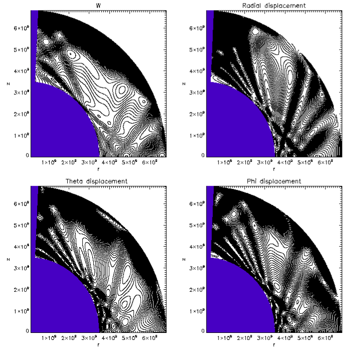
Figure 13: As in Figure 10 but for the model with a core radius of $0.5R_{*}$ at $t=0.589days.$

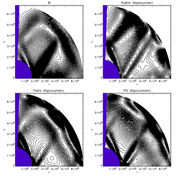
Figure 14: As in Figure 9 but for a model with core radius $0.25R_{*},$ $\Omega/\Omega_{*}=0.36$ and $\eta=8\sqrt{2}$ at $t=2.326days$, which is after the encounter. Contour line plots illustrate the inertial wave propagation pattern

The energy transferred to the planet as a function of time due to the $m=2$ tide is shown in Figure 7 for a model with a solid core of radius $0.25R_{*}$ for $\eta=4$ and $\Omega/\Omega_{*}=0.8.$ Simulations have been performed with resolutions of $200\times 200$ and $400*400.$ The results agree closely with some small additional dissipation in the lower resolution case, which is to be expected. Interestingly, the energy transferred to the planet is almost the same in the cases with and without a core. This transfer is less in magnitude than in the non rotating case, which gives almost identical results to those found for the non rotating coreless case.

The corresponding angular momenta transferred to the planet are plotted as a function of time in Figure 8. As for the energy transferred, the angular momentum transferred in this model and the coreless model are very similar.

The global response pattern after $t=0.408days$ is illustrated in Figure 9. This is shortly before the end of the encounter. Although there is evidence for some small scale structures developing near the core boundary, the basic response appears global with little evidence of critical latitude phenomena or wave attractors. However, this appears at later times. Response pattern contours are shown in Figure 10 at $t=0.77{\rm days},$ being well after the end of the encounter. Localised inertial wave propagation and reflection patterns are clearly visible. As expected these present a constant angle of propagation to the vertical and graze the core boundary.

The fact that the development of these structures occurs at late times is indicative of why the coreless and cored results agree in this case. We note that this may be expected when the time scale for the encounter is not long compared to the rotation period. In such a case there would not be adequate time for inertial waves to propagate, reflect and develop structures indicating shear layers or attractors. This might be expected to be especially the case when the core is small and so presents a small target for propagating waves. Physically, as far as the inertial mode excitation is concerned, the encounter would appear impulsive in which case the energy and angular momentum transfers should not be affected by the later development of shear layers or wave attractors. Therefore, as long as the core is not too large we expect the same result as for a coreless model. These ideas are developed from a mathematical point of view in appendix B. Although the encounter time scale and rotation period are comparable in this case, in accordance with the above discussion, we do not see the development of wave propagation patterns until the late stages of the encounter, and the cored and coreless model energy and angular momentum transfers are very similar.

3.4.2 A planet with core radius equal to $0.5R_{*}$

We have also performed simulations a model with a solid core of radius $0.5R_{*}.$ Again the encounter was for $\eta=4$ and $\Omega/\Omega_{*}=0.8.$ The energy and angular momentum transferred as a function of time are shown in Figures 11 and 12, respectively. Results are given for resolutions of $400\times 400$ and $800\times 800.$ These agree closely but with again more dissipation in the lower resolution case. In contrast to the case of the smaller core the energy transferred is larger than in the coreless case by a factor of $\sim 8-9.$ This is probably because the larger core enabled a wave structure to develop faster. To illustrate the wave pattern, contour plots of the response are shown in Figure 13 at $t=0.59days$, which is shortly after the encounter. These appear to be of a similar form to, but somewhat more intricate than the model with a smaller core.

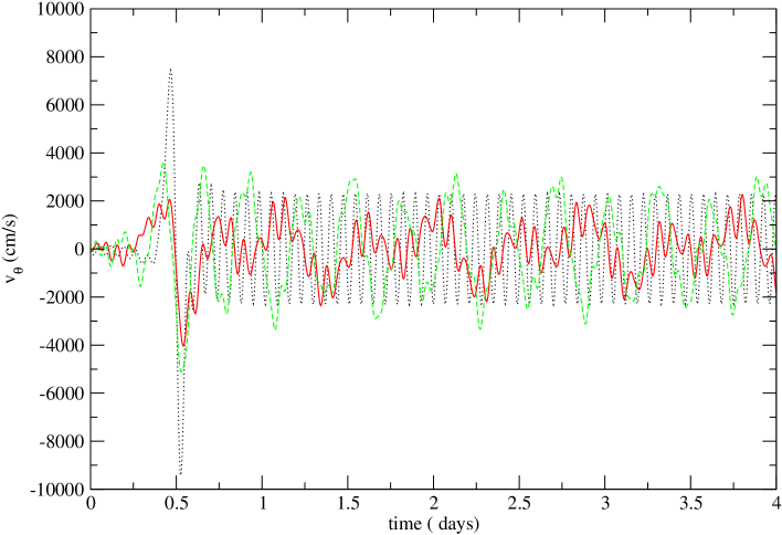
Figure 15: The real part of the $\theta-$component of velocity in an inner point of the planet as a function of time, $\eta=4\sqrt{2}$ and $m=2$ for these tidal encounters. Simulations for $\Omega/\Omega_{*}=0,0.24$ and $0.36$ are plotted with dotted, solid and dashed curves, respectively.

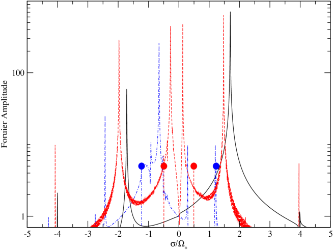
Figure 16: Fourier spectra obtained by the Fourier transform of the velocity data as functions of the ratio $\sigma/\Omega_{*}$ for $\eta=4\sqrt{2}.$ The case $m=2$ is shown. The solid (black) curve corresponds to the non-rotating case $\Omega=0$ while the dashed (red) and dash-dotted (blue) curves are for $\Omega/\Omega_{*}=0.24$ and $0.6$ respectively. The vertical lines delimit the range of $\sigma$, where inertial modes are theoretically possible, with line styles identical to those used for corresponding values of $\Omega.$

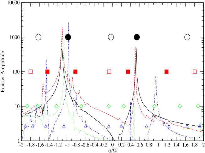
Figure 17: The Fourier spectra as functions of the ratio $\sigma/\Omega$, with only the range corresponding to the inertial branch of pulsations $|\sigma/\Omega|\leq 2$ explicitly shown, for $m=2$ and $\eta=4\sqrt{2}$. The solid (black), dashed (red) , dotted (green) and dot-dashed (blue) curves are for $\Omega/\Omega_{*}=0.24,0.36,0.6$ and $1.0.$ Note that the latter case is unrealistic but included for completeness. The symbols show positions of the WKBJ modes obtained in IPN, with different style corresponding to different WKBJ mode order, $l$. The circles, squares, diamonds and triangles are for $l=1,2,3$ and $4$, respectively.

3.4.3 Cored models for slower rotation and larger $\eta$

In order to indicate that the results described above are not radically altered when $\Omega$ is reduced and $\eta$ is increased, we also simulated cored models with $\eta=8\sqrt{2}$ and $\Omega/\Omega_{*}=0.36.$ The models with core radii $0.25R_{*}$ and $0.5R_{*}$ behaved very similarly, in relation to their coreless counterparts, to those described above for larger $\Omega$ and smaller $\eta.$ Figure 14 illustrates the wave propagation pattern that results from the encounter when the core radius was $0.25R_{*},$ which is indeed similar to that found for the cases with larger rotation.

4 A comparison of the numerical, spectral and WKBJ approaches

4.1 Normal mode frequencies obtained from the simulations and their comparison with the basis function and WKBJ approaches

Here we investigate the spectrum of normal modes excited in the above simulations determined from fast Fourier transform of the time series. We compare the derived inertial mode frequencies with the results obtained in IPN.

As time series used for our Fourier analysis, for definiteness, we consider the time dependence of the real and imaginary parts of the ${\theta}-$component of velocity at an inner point of the planet, with $r=4.8\times 10^{9}cm$ and $\theta=67$ degrees, after a tidal encounter with $\eta=4\sqrt{2}$, for different values of the angular velocity $\Omega$. This is shown in Fig. 15 for $\Omega/\Omega_{*}=0.24$ and $0.36$. The sharp change occurring around $0.5$ day is due to the tidal encounter itself, the pulsation modes are generated during this period of time. After approximately $1$ day the influence of the perturbing tidal field becomes unimportant and the planet’s perturbation becomes quasi-periodic. As follows from Fig. 15, in the case of the non-rotating planet, only one relatively short period of pulsation can be clearly seen. This is the period of the fundamental prograde mode. When the planet rotates several periods can be seen with one short period corresponding to the fundamental mode together with several relatively long periods determined by presence of inertial modes in the spectrum.

To obtain the Fourier transforms we removed the first part of the data series to eliminate the contribution of direct forcing by the tidal field, typically of duration $5\times 10^{4}-10^{5}s$. The results are presented in Figs. 16-18. In Fig. 16 we compare the spectrum obtained for the non-rotating planet with those obtained for the rotating cases, for $m=2$. The spectra are plotted as functions of the ratio $\sigma/\Omega_{*}$, where $\sigma$ is the frequency. The peaks in Figure 16 correspond to positions of normal modes. The black curve represents the results obtained for $\Omega=0$. The positions of the two peaks are symmetric about $\sigma=0,$ though the peak amplitudes are not. This is because the prograde modes with positive values of $\sigma$ are excited much more effectively than the retrograde modes, for a non-rotating planet . The prominent peaks with $\sigma\approx\pm 1.6\Omega_{*}$ give the positions of the fundamental mode. Note that their eigenfrequencies are larger than those calculated for the same planet model but without the Cowling approximation. The peaks with larger values of $\sigma/\Omega_{*}$ give the positions of p-modes (pressure waves). Note the absence of any peaks in between the two peaks corresponding to the fundamental mode. This is because there is no branch of low frequency oscillations in a non-rotating barotropic planet. When the planet rotates the peaks corresponding to fundamental modes are shifted leftwards, with the magnitude of the shift proportional to $\Omega$. This effect is briefly discussed below.

The most notable difference between the non-rotating case and the rotating ones is the presence of peaks in between the two peaks corresponding to the fundamental modes in the rotating cases. These are the peaks corresponding to the inertial modes. Note that all these peaks lie within the theoretical range allowed for inertial waves $|\sigma\leq 2\Omega|.$ This range is marked by vertical lines with styles corresponding to those associated with the corresponding angular velocity. For small values of $\Omega$, significantly less than the largest value $\Omega/\Omega_{*}=0.6$ shown in Fig. 16 , there are two notably large peaks within the inertial range, one with a positive and one with a negative value of $\sigma$. These are identified with two main global modes discussed in detail in PI, IP and IPN. From the point of view of the WKBJ theory developed in IPN, these modes correspond to smallest value of an integer $l$ classifying WKBJ modes, called the WKBJ order later on. In the case of $\Omega/\Omega_{*}=0.6,$ represented by the dot-dashed curve, there is a third noticeable peak close to $\sigma\approx 2\Omega$ and within the inertial mode range. It is the prograde fundamental mode, which has been shifted within this frequency range by rotation. A number of peaks with smaller amplitudes give the positions of higher order inertial modes.

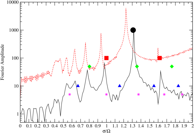
Figure 18: Same as Fig. 17 but for the case $m=0$, $\eta=4$. Since in this case the spectra are symmetric about the origin $\sigma=0$ only the positive values of $\sigma$ within the inertial range $\sigma/\Omega\leq 2$ are shown. $\Omega/\Omega_{*}=0.36$ for the solid (black) curve and $\Omega/\Omega_{*}=0.8$ for the dashed (red) one. Symbols show the positions of $WKBJ$ modes. Note that the WKBJ mode order $l$ runs starting from $l_{min}=0$ in this case. The black circles, red squares, green diamonds, blue triangles and magenta stars are for $l=0,1,2,3$ and $4$, respectively.

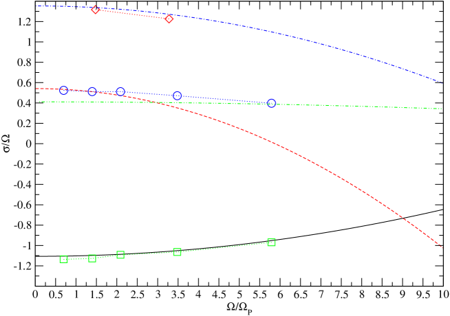
Figure 19: Eigenfrequencies $\sigma/\Omega$ of a few ’global’ inertial modes as functions of the ratio $\Omega/\Omega_{p}$, where $\Omega_{p}$ is is a typical frequency of periastron passage, see equation (25). The dot-dashed curve having $\sigma/\Omega\approx 1.3$ when $\Omega\rightarrow 0$ is the analytical curve for the axisymmetric $m=0$ global $l=2$ mode. The curves having $\sigma/\Omega\approx 0.5$ and $-1.1$ when $\Omega\rightarrow 0$ are for the global $l=1$ $m=2$ modes, while the curve with $\sigma/\Omega\approx 0.4$ is for the next order $l=2$ curve. Symbols joined by dotted lines represent the corresponding results of numerical calculations. One can see that the agreement between the numerical and analytical results for the global $m=0$ mode and the global $m=2$ mode with negative values of $\sigma$ is quite good. The analytical results for the global $m=2$ mode with positive values of $\sigma$ agree with the numerical ones only when $\Omega$ is sufficiently small. In the opposite case of large values of $\Omega$ the numerical results are close to the analytical curve for the next order $m=2$ $l=2$ mode. This result may be explained by the effect of avoided crossing.

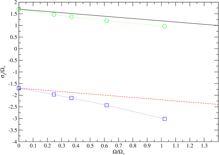
Figure 20: Eigenfrequencies $\sigma/\Omega_{*}$ of $m=2$ fundamental modes as functions of the ratio $\Omega/\Omega_{*}$. The solid and dashed curves represent the theoretical results for the prograde and retrograde mode, respectively. Symbols joined by the dotted lines represent the results of numerical calculation. One can see that the agreement between the theoretical and numerical results is much better for the prograde mode. Note that the same phenomenon was observed in numerical calculations of normal modes of rotating polytropic stars, which do not use the Cowling approximation, ( see eg. Managan 1986).

The eigenfrequencies of inertial modes are naturally expressed in units of $\Omega$ and we show the part of the spectrum within the inertial range as a function of the ratio $\sigma/\Omega$, for the case $m=2$ in Fig. 17 and for the case $m=0$ in Fig. 18. Additionally, we show positions of WKBJ modes calculated in IPN by symbols with larger values of symbol ordinates and sizes corresponding to smaller values of the WKBJ order $l$. As was discussed in IPN among the WKBJ modes with the same value of $l$ there are modes, which were not identified with results obtained by other methods. These modes are situated close to boundaries of the allowed region $\sigma=\pm 2\Omega$ as well as close to the origin $\sigma=0$. The theory developed in IPN is likely to be beyond limit of its applicability close to the boundaries and to the origin $\sigma=0$. We expect that these unidentified modes could be absent in a more advanced WKBJ theory. Therefore, we do not show positions of modes having most negative, most positive and the smallest values of $\sigma$, for a given value of $l$.

In Fig. 17 the case of $m=2$ is shown. The solid black and dashed red curves correspond to the cases of relatively small $\Omega/\Omega_{*}=0.24$ and $0.36,$ which should be compared with WKBJ results obtained in the anelastic approximation. Two global modes are clearly seen with their positions in a close agreement with positions of the WKBJ modes having the smallest value of $l_{min}=1$ for $m=2.$ The WKBJ modes corresponding to $l=2$ and $3$ are also shown. Their positions are close to some numerically obtained peaks, notably in the case of the $l=2$ modes having the ratio $\sigma/\Omega$ close to $-1.5$, $-0.8$ and $1.25$. The fact that some of the next order WKBJ modes are not seen in the numerical data is not worrying since the amplitude of modes excited after the tidal encounter depends of the shape of the Fourier transform of the dependence of the tidal potential on time, which, in its turn, depends very sensitively on the value of $\Omega,$ see PI and IP. With increase of $\Omega$ the retrograde modes with negative values of $\sigma$ are excited more efficiently and their amplitude grows, see Figure 17. In the case of the largest considered value of $\Omega=\Omega_{*}$ the peaks corresponding to the retrograde mode with $l=1$ and $2$ are strongly amplified, and the peaks close to $\sigma/\Omega=-1.7$ and $-0.7$ may be identified with the WKBJ modes having $l=3$. Also, the peaks are shifted towards the origin $\sigma=0$ as $\Omega$ increases, an effect which may be explained by corrections to the anelastic approximation, see IPN and below. In the cases of $\Omega/\Omega_{*}=0.6$ (the dotted green curve) and $\Omega/\Omega_{*}=1$ (the dot-dashed blue curve) there is an additional noticeable peak with a positive value of $\sigma$. This corresponds to the prograde fundamental mode being shifted into the inertial range due to rotation.    
In Fig. 18 we show the case $m=0$. Since in this case the spectra are symmetric about $\sigma=0$ only positive frequencies within the inertial range $\sigma<2\Omega$ are considered. Similar to the previous case symbols show positions of the WKBJ eigenmodes calculated by IPN. As in Fig. 16 larger ordinates correspond to smaller values of the WKBJ order $l$ with the smallest $l=l_{min}=0$ denoted by circles and the eigenfrequencies of modes with largest shown $l=4$ denoted by stars. We see from Fig.18 that the peak with largest amplitude has a value of $\sigma$ close to the identified main global mode with $l=0$ and $\sigma\approx 1.3\Omega$. Two identified WKBJ modes at the next order, also have well pronounced peaks with positions close to the values of their eigenfrequencies. One can also possibly identify the eigenfrequencies corresponding higher order modes with some peaks with smaller amplitude, especially in the region $0.5<\sigma/\Omega<1$, where there is seemingly a good agreement between positions of the peaks and eigenfrequencies of modes having $l\leq 6$. When rotation of the planet increases the positions of the peaks are shifted to smaller values of $\sigma$. This agrees with results obtained in IPN, see also below.

4.1.1 Change of eigenfrequencies with $\Omega$

In the anelastic approximation which is frequently used for calculations of eigenspectra of modes belonging to the inertial branch, the mode frequencies are proportional to $\Omega$. This approximation is not, however, exact, and it discards certain terms proportional to $(\Omega/\Omega_{*})^{2}$ in the set of equations describing pulsations, see eg. IPN for discussion. In IPN a correction to the mode eigenfrequencies due to terms not accounted for in the anelastic approximation was calculated. It was shown that in the linear approximation in the small parameter $(\Omega/\Omega_{*})^{2}$ and neglecting a possible mode mixing, the eigenfrequencies have the form

$$\sigma_{i}=\sigma^{a}_{i}+\alpha_{i}(\Omega/\Omega_{*})^{2}\Omega,$$ (9)

where $\sigma_{i}^{a}$ is the value of a certain eigenfrequency calculated in the anelastic approximation and an explicit expression for dimensionless parameter $\alpha_{i}$ can be found in IPN. We calculate $\alpha_{i}$ for three modes corresponding to the case $m=2$ using results obtained in PI and IP. For the main retrograde global mode having $l=l_{min}=1,$ from the viewpoint of the WKBJ method, the eigenfrequency $\sigma^{a}_{1}\approx-1.1\Omega$ and $\alpha_{1}\approx 0.15$. For the prograde $l=1$ main global mode we have $\sigma^{a}_{2}\approx 0.54\Omega$ and $\alpha_{2}\approx-0.5$, and for the next order $l=2$ mode which has a close value of the eigenfrequency $\sigma_{3}\approx 0.41\Omega$ we get $\alpha_{3}\approx-0.022$. Additionally, we calculate the correction for the $m=2$ main global mode with $l=l_{min}=2$, which has $\sigma_{1}\approx 1.35\Omega$ and $\alpha_{1}\approx-0.12$. Then, the value of $\sigma_{i}$ given by equation (9) is compared with what is obtained in the numerical calculations. The results of this comparison are presented in Figure 19. Note that for the curves corresponding to $m=2$ the parameter $\eta=4\sqrt{2}$ while in the case $m=0,$ $\eta=4$, and we recall that $\eta=\Omega_{*}/\Omega_{p}$, where $\Omega_{p}$ is is a typical frequency of periastron passage explicitly defined in equation (25) of appendix A. As seen from Fig.19 there is good agreement between the numerical results and those calculated with help of equation (9) for the $m=0$ global mode and the retrograde $m=2$ global mode. In the case of the prograde $m=2$ global mode only two numerical points with $\Omega/\Omega_{p}<1.5$ are in agreement with the analytical result. For larger rotation rates the numerical curve deviates from the analytical one calculated for the global mode. Instead, it approaches the analytical curve calculated for the next order $l=2$ mode in the limit of large rotation. Since the theoretical curves corresponding to the global mode and the $l=2$ mode intersect each other at $\Omega/\Omega_{p}\approx 3$, the fact that at larger rotation rate the numerical results are closer to the curve describing the $l=2$ mode may be explained by the phenomenon of avoided crossing. The global and the next order mode lose their identity at these rotation rates, being in mixed states with mode mixing provided by an operator describing the correction to the anelastic approximation, see IPN for its explicit form.

Now let us shortly discuss the behaviour of the fundamental modes with change of rotation rate. In order to find the corresponding analytical estimate of change of eigenfrequencies we should remember that we work in the rotating frame while the fundamental modes are normally studied in the inertial frame. In the latter frame there is a simple expression for a correction of the mode eigenfrequency, $\sigma_{f}$, due to rotation

$$\sigma_{f}-\sigma^{nr}_{f}=m\beta\Omega,$$ (10)

where $\sigma_{f}^{nr}$ is the frequency of a fundamental mode calculated for a non-rotating planet, and $\beta$ is determined by some integral over the planet’s volume, see eg. Cristensen-Dalsgaard and references therein. As was shown by eq. Ivanov $\&$ Papaloizou 2004 $\beta\approx 0.5$ for planetary models, which are close to the standard $n=1$ polytrope. Eigenfrequencies associated with the rotating frame are shifted with respect to the ones in the inertial frame according to the rule $\sigma\rightarrow\sigma-m\Omega$. Therefore, in the rotating frame, for the case of the $m=2$ mode, we obtain a simple relation

$$\sigma_{f}=\sigma^{nr}_{f}-\Omega,$$ (11)

where we set $\beta=0.5$. This relation is compared with the numerical results in Fig. 20. One can see from Fig.20 that the numerical and analytical approaches are in a good agreement for the prograde mode while in the case of retrograde mode the results differ. The fact that the simple approximation (11) doesn’t work well for the retrograde fundamental modes, for finite values of rotation rates, has been known for quite a long time, see eg. Managan (1986). Since this issue is not directly relevant to the purposes of this paper we do not discuss it in more detail here.

5 Coreless models under a fixed quadratic potential

Goodman & Lackner (2009) considered special barotropic models which are in hydrostatic equilibrium under a fixed quadratic gravitational potential $\Psi$ in the unperturbed state. Thus

$$\frac{1}{\rho}\frac{dP}{dr}=\frac{c^{2}_{s}}{\rho}\frac{d\rho}{dr}=-\frac{d\Psi}{dr},$$ (12)

with $\Psi=c_{1}+c_{2}r^{2},$ with $c_{1}$ and $c_{2}$ being constant. Such models have a special property in common with the uniform density model that $(1/\varpi)\partial\Psi/\partial\varpi=(1/r)d\Psi/dr=c_{2}\equiv\omega_{0}^{2}$ is constant. Such spherically symmetric models may be found for an arbitrary specified density distribution if the pressure is allowed to be determined a posteriori by the condition for hydrostatic equilibrium.

Goodman & Lackner (2009) showed that these models had the property that when full compressibility was retained, no inertial modes are excited by a quadrupole $m=2$ tidal potential. Thus for these models the response is determined entirely by the $f$ modes. In appendix C we review the compressible case and show that no inertial modes are excited when the anelastic approximation we use is employed. Thus no spurious inertial mode excitation occurs as a result of its use for these models. Nonetheless it is important that the numerical schemes we employ correctly represent the tidal excitation of these models. This we demonstrate below for the finite difference approach adopted in this paper. The situation with respect to the spectral approach adopted in previous papers, which is also found to behave correctly is discussed in appendix C.

5.1 Simulations with quadratic potential models

The models that we have adopted in order to compare their tidal response to that of the standard polytropic model considered in this paper have the same mass and radius as but a density distribution that depends quadratically on radius. The central density is given by

$$\rho_{c}=\frac{15M_{*}}{8\pi R_{*}^{3}}$$ (13)

This is smaller than the corresponding value for the polytrope in equilibrium under a self-consistent gravitational potential given in appendix A because the quadratic potential model is less centrally condensed. The central pressure is given by

$$P_{c}=\frac{15GM_{*}^{2}}{32\pi R_{*}^{4}}.$$ (14)

The density and pressure in the interior are then respectively given by $\rho=\rho_{c}(1-r^{2}/R_{*}^{2})$and $P=P_{c}(1-r^{2}/R_{*}^{2})^{2}.$ Thus this model also satisfies the equation of state for a polytrope with index $n=1.$ However, hydrostatic equilibrium confirms that this is a quadratic potential model with potential determined to within an arbitrary constant by $\Psi=GM_{*}r^{2}/(2R_{*}^{3}).$

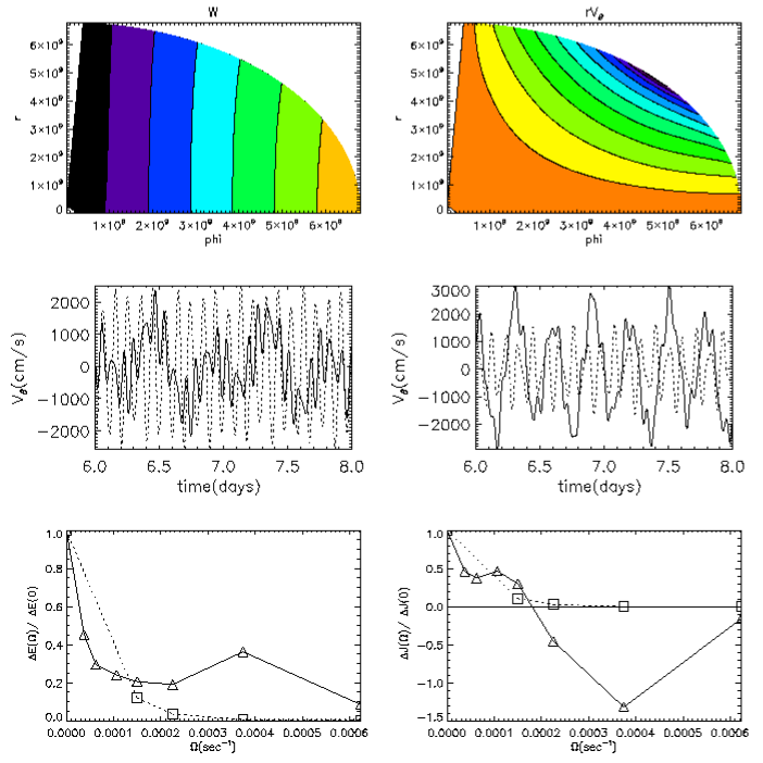
Figure 21: This figure illustrates the behaviour of the quadratic potential models discussed in the text with some comparisons to a corresponding standard polytropic model for encounters with $\eta=4\sqrt{2}.$ The left uppermost panel gives contours of the real part of $W$ and the right uppermost panel contours of the real part of $rv_{\theta}$ $13.38$ days after pericentre passage for the quadratic potential model with $\Omega/\Omega_{*}=0.36.$ The central panels give the real part of $v_{\theta}$ evaluated at $r=4.8\times 10^{9}cm$ and $\theta=67$ degrees as a function of time between six and eight days after pericentre passage. The left central panel illustrates the standard polytropic model (solid curve) and the corresponding quadratic potential model (dashed curve) for $\Omega/\Omega_{*}=0.24.$ The right central panel illustrates the same quantities for $\Omega/\Omega_{*}=0.36.$ The lowermost left panel shows the energy transferred from the orbit relative to its value for $\Omega=0$ as a function of $\Omega$ in sec${}^{-1}.$ We recall that $\Omega_{*}=6.23\times 10^{-4}$ sec ${}^{-1}.$ The standard polytrope is illustrated with the solid curve and the quadratic potential model with the dotted curve. The lowermost right panel gives the corresponding plot for the angular momentum transferred from the orbit.

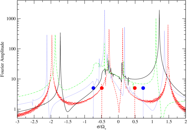
Figure 22: This shows a comparison of the Fourier spectra obtained by the Fourier transform of the velocity data as functions of the ratio $\sigma/\Omega_{*}$ for $\eta=4\sqrt{2}$ for standard polytropic and corresponding quadratic potential models. The case $m=2$ is shown. The solid (black) curve corresponds to the quadratic potential model with $\Omega/\Omega_{*}=0.24$ while the dashed (red) curve is for the corresponding polytropic model. The dash-dotted (green) curve is for the quadratic potential model with $\Omega/\Omega_{*}=0.36$ and the dotted (blue) curve is for the corresponding polytropic model. The vertical lines delimit the range of $\sigma$, where inertial modes are theoretically possible, with line styles identical to those used for corresponding values of $\Omega.$

	$f_{+a}$	$f_{+n}$	$f_{-a}$	$f_{-n}$
$\Omega/\Omega_{*}$	$\sigma/\Omega_{*}$	$\sigma/\Omega_{*}$	$\sigma/\Omega_{*}$	$\sigma/\Omega_{*}$
$0$	1.4142	1.4154	-1.4142	-1.4154
$0.24$	1.1940	1.1965	-1.6750	-1.6751
$0.36$	1.0988	1.0990	-1.8202	-1.8222

Table 1: A comparison between $f$ mode angular frequencies obtained from numerical simulations with analytically determined values. The first column gives the angular velocity, the second and third columns give the analytic and numerical prograde $f$ mode angular frequencies respectively. The fourth and fifth columns give the corresponding quantities for the retrograde $f$ mode.

We have performed simulations of quadratic potential models for $\eta=4\sqrt{2}$ for a number of rotation frequencies and a resolution $200\times 200$ that can be directly compared to those for the corresponding standard polytropes with $n=1$ (the global simulation parameters for the different models are the same). In particular, we establish that although there is some mild distortion due to the form of the computational grid and numerical truncation, that causes some weak inertial mode excitation, the response of the quadratic potential models is determined by the $f$ modes as expected. Some numerical results for these simulations are shown in Fig. 21.

The lowermost left panel shows the energy transferred from the orbit as a function of $\Omega$ relative to its value for $\Omega=0.$ The lowermost right panel gives the corresponding plot for the angular momentum transferred from the orbit. We remark that when $\Omega=0,$ the energy and angular momentum transfers for the quadratic potential models exceed those for the polytropic models by factors of $9.2$ and $11.0$ respectively, because the polytropic models are more centrally condensed. The lack of inertial mode response is apparent in the quadratic potential models which do not show the related increase in energy transfer for intermediate values of $\Omega.$ The interaction is much weaker for intermediate and larger values of $\Omega$ for these models. This is also indicated when one considers the value of $\Omega$ for which the angular momentum transfer is zero. This defines the angular velocity $\Omega_{ps}$ for which pseudo synchronisation is achieved (Ivanov & Papaloizou 2004, IP).

The angular velocity for pseudo synchronisation taking account only $f$ modes was estimated in general by Ivanov & Papaloizou (2004) to be given by

$$\Omega_{ps}=\frac{(2+\ln(\eta))\Omega_{*}}{\eta}.$$ (15)

However, when inertial modes are taken into account IP find that $\Omega_{ps}\sim 1.55\Omega_{*}/\eta.$ Thus, assuming $f$ modes dominate the quadratic potential models and inertial modes dominate the polytropic models, for the simulations illustrated in Fig. 21, we expect $\Omega_{ps}=071\Omega_{*}$ in the former case and $\Omega_{ps}=0.27\Omega_{*}$ in the latter. For the numerical results plotted in Fig. 21, $\Omega_{ps}\sim 0.6\Omega_{*}$ and $\Omega_{ps}\sim 0.29\Omega_{*}$ for these quantities respectively. As the estimates of Ivanov & Papaloizou (2004) and IP assumed $\Omega$ to be small, this agreement is satisfactory and implies consistency with the view that the polytropic models are inertial mode dominated and the quadratic potential models $f$ mode dominated.

The form of the tidally excited disturbance in the quadratic potential model with $\Omega/\Omega_{*}=0.36$ $13.38$ days after pericentre is illustrated in the uppermost panels of Fig. 21. The same form is seen at other times long enough after the tidal encounter. Contours of the real parts of $W$ and $rv_{\theta}$ are shown. The former are approximately vertical as expected from the analytic form $W\propto\varpi^{2}$ (see appendix C) and the latter are approximately hyperbolae corresponding to the expected form $rv_{\theta}\propto\varpi z.$

The central panels of Fig. 21 give the real part of $v_{\theta}$ as a function of time at an inner point of the planet, with $r=4.8\times 10^{9}cm$ and $\theta=67$ degrees, between six and eight days after pericentre passage both for the standard polytropic model and the corresponding quadratic potential model for $\Omega/\Omega_{*}=0.24$ and $\Omega/\Omega_{*}=0.36.$ It will be seen that the quadratic potential model responses show high frequency behaviour corresponding to excitation of the $f$ modes whereas the corresponding polytropic models show in addition a dominant contribution from longer period disturbances that are associated with inertial modes.

In order to better quantify this we have performed a Fourier analysis of longer spans of these time series in order to determine the mode spectra for these cases. The results are plotted in Fig. 22. From this figure it is apparent that when corresponding models are compared the inertial mode amplitudes are an order of magnitude or more smaller for the quadratic potential models, corresponding to a mode energy a hundred times or more smaller. For the standard polytropic cases plotted, the response is dominated by the inertial modes in contrast to the $f$ mode dominated quadratic potential models.

As an additional test we compare the numerically determined $f$ mode frequencies for the quadratic potential models to the analytically determined values. For the quadratic potential models the $f$ mode angular frequencies are given by $\sigma=-\Omega\pm\sqrt{2\omega_{0}^{2}+\Omega^{2}}$ (Goodman & Lackner 2009). Here the positive sign corresponds to the prograde mode and the negative sign to the retrograde mode. We compare these values to the numerical values we obtained from the spectral analysis of the time series indicated above for $\Omega=0,\Omega/\Omega_{*}=0.24$ and $\Omega/\Omega_{*}=0.36$ in table 1. The numerical and analytic values correspond to within a relative discrepancy of $2\times 10^{-3}$ and so are in good agreement. We conclude that our numerical treatment adequately represents the $f$ modes and their dominance of the tidal response for the quadratic potential models.

Figure 23: The dimensionless quantities $\epsilon$ and $\lambda$ determining the energy transfer in the rotating frame and the angular momentum transfer, respectively, are plotted as functions of $\Omega/\Omega_{p}$. The case of a tidal encounter having $\eta=4\sqrt{2}$ is shown. The uppermost solid, dashed and dotted curves describe results of theoretical calculation of $\epsilon$ while the corresponding lowermost curves determine theoretical values of $\lambda$. Symbols represent the results of numerical calculations. The solid curves are calculated with all inertial and fundamental modes accounted for, the frequency corrections to the fundamental modes given by equation (11) and to two main global modes given by equation (9) are taken into account as well. The dashed curve differ from the solid ones by the fact that only the two main global modes are taken into account in the expressions determining the contribution of the inertial modes. The dotted curves show the case when the contribution of the fundamental modes as well as the frequency corrections are neglected and only two main global inertial modes are taken into account. Note that the dotted curves do not depend on value of $\eta$. These curves are, therefore, called ’the universal curves’ later on.

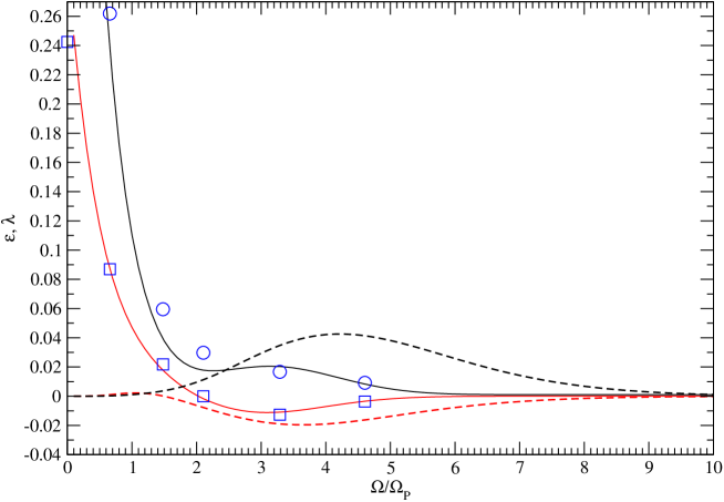
Figure 24: Same as Fig. 23 but for a closer encounter with $\eta=4$. For simplicity only two mail global modes are taken into account in the expressions determining the energy and angular momentum transfer due to inertial waves. Both contributions of the fundamental modes and of inertial modes as well as the corresponding frequency corrections are used to calculate the solid curves while the dashed curves are the universal ones.

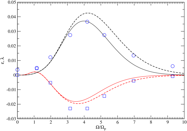
Figure 25: Same as Fig. 24 but for a more distant encounter with $\eta=8\sqrt{2}$.

6 Comparison of the energy and angular momentum transfer with the results obtained by the spectral methods

6.1 Numerical simulations versus the spectral approach

Let us compare the energy and angular momentum transferred for individual simulations with results obtained from the basis function (or spectral) approach developed in PI and IP. The expressions for energy and angular momentum transfer determined by the inertial modes, $\Delta E_{m}$ and $\Delta L_{2}$ obtained by PI in the anelastic approximation are for convenience reproduced in appendix B, see equations (29) and (30). Let us recall that $m$ is the azimuthal mode number. As we discussed above the numerical results show that modes with $m=0$ give a negligible contribution to the energy transfer, and, therefore, we set $m=2$ later on. Also note that the quantity $\Delta E_{2}$ is defined in the rotating frame. The energy transfer in the inertial frame is given as $\Delta E_{I}=\Delta E_{2}+\Omega\Delta L_{2}$. Contrary to $\Delta E_{2}$, $\Delta E_{I}$ can be negative.

It follows from equations (29) and (30) that dimensionless quantities

$$\epsilon=\eta^{6}\Delta E_{2}/E_{*}\quad\lambda=\eta^{5}\Delta L_{2}/L_{*}$$ (16)

depend only on the dimensionless ratio $\Omega/\Omega_{p}$ in the anelastic approximation. Therefore, they conveniently represent the energy and momentum transferred and we compare these quantities with what is given by numerical calculations below. In our spectral approach we use the results obtained by IP to calculate the overlap integrals (see equation (31) for the definition) and eigenfrequencies, for their model of a cold Jupiter with smoothed density jump in a place of phase transition between molecular and metallic hydrogen, as this model is like a standard polytrope with index $n=1.$ Formally, the quantities $\epsilon$ and $\lambda$ are given by infinite summation series over all eigenmodes with $m=2$. In practice, the number of modes is limited by the resolution of the numerical method used , which in turn is determined by the number of basis functions in the case of a spectral method. As we mentioned above, in the calculations of PI and IP $225$ basic functions were used giving $450$ eigenfrequencies. However, as was mentioned by PI and IP only two main global modes (a prograde one with $\sigma\approx 0.5\Omega$ and a retrograde one with $\sigma\approx-\Omega$ give the main contribution to the transfer of energy and angular momentum, for small and moderate ratios of $\Omega/\Omega_{p}$. Thus, to compare the results obtained by different methods we consider two approaches: the first takes into account all of the eigenmodes available in the spectral method, the second takes into account only the contributions of the two main global modes.

In order to compare the spectral and numerical results we should add to the expressions (16) the corresponding contributions arising from excitation of the fundamental modes, for a rotating planet. These have been derived in Ivanov $\&$ Papaloizou 2004 (see also Lai 1997). Additionally, we take into account the frequency correction (9). After these modifications are made, the expressions (16) acquire dependence on $\eta$. To emphasise the difference between the expressions with and without these modifications we call the latter ’universal curves’.

The results of the comparison of $\epsilon$ and $\lambda$ are presented in Figures 23-25. In Fig. 23 we show the case of a tidal encounter with $\eta=4\sqrt{2}$. The solid and dashed curves represent the results given by the spectral method with the contribution of the fundamental modes as well as the frequency corrections included while the dotted curves are the universal ones. The symbols show the results of numerical calculations. One can see that the agreement between the spectral and analytical approaches is quite good apart, possibly a region with $\Omega/\Omega_{p}\approx 1.5$. In particular, it is clear from Fig.23 that for a sufficiently small ratio $\Omega/\Omega_{p}<1.5$ the energy and angular momentum gained by the planet are determined by excitation of the fundamental modes while in the opposite case the inertial waves dominate the tidal response. Therefore, eg. the curve giving the energy transferred to the planet has non-monotonic shape. Initially it decreases with $\Omega/\Omega_{p}$ due to suppression of the contribution determined by the fundamental modes caused by increase of rotation, then it starts to increase due to increasingly more efficient excitation of the inertial waves attaining a maximum at $\Omega/\Omega_{p}\sim 3.5$, then it decreases again. One can also see that the role played by the frequency corrections to the inertial modes is essential with the universal curves giving much worse agreement with the numerical results in the region, where the inertial waves dominate. On the other hand it is difficult to see whether the curve with all inertial eigenmodes taken into account (the solid curve) or the curve determined by two main global modes (the dashed curve) gives a better approximation to the numerical data. We expect that in order to differentiate between these two curves even larger rotation rates should be considered. This issue is briefly discussed below, where we compare results of the spectral and WKBJ methods. In the rest of this section we consider only two main global modes in the expressions for the tidal transfer due to inertial waves.

In Fig. (24) the case of a stronger tidal encounter with smaller value of $\eta=4$ is considered. As in the previous case the agreement is very good. As expected the role of the fundamental modes is more important at small rotation rate while the role of the frequency corrections becomes quite important at large values of rotation.

Fig. (25) shows the case of relatively weak tidal encounter with $\eta=8\sqrt{2}$. In this case the inertial waves dominates the tidal response for all non-zero rotation rates considered. Also, the role played by the frequency corrections is minor relative to the previous case, and, therefore, the curves taking these ones into account are close to the universal curves in this case. Note that the numerically obtained value of $\epsilon$ is larger than the theoretical value for the maximal $\Omega/\Omega_{p}\approx 9$. This might possibly be explained by contributions of higher order WKBJ modes to the energy transfer, which are not taken into account in the theoretical curve.

7 Discussion

In this paper we extended our previous work (IP) on the tidal interaction of a planet on a highly eccentric or parabolic orbit about a central star by relaxing the anelastic approximation and considering the tidal response of planet models with solid cores. These changes were accomplished by carrying out numerical simulations of tidal encounters considered as initial value problems. The response of $f$ and $p$ modes was found in addition to that due to low frequency inertial modes.

We calculated the energy and angular momentum exchanged after pericentre passage for a variety of pericentre distances and angular velocities of rotation of the planet. Models both with and without a solid core were simulated. In the latter case the state variables showed evidence of the emission of shear layers and/or wave attractors after the encounter.

In the coreless case we studied the spectrum of excited inertial modes and compared it with the spectra obtained in IP and with the analytic theory described in IPN. We found good agreement for slow rotation. We were also able to account for the variation of the normal mode frequencies with the planet’s angular velocity. In the case of inertial waves a non-trivial variation is induced by terms neglected in the anelastic approximation and it is found to be small for rotation frequencies significantly less than critical. Thus our analysis indicated that this approximation is generally a valid one for the inertial modes.

We presented results for the total energy and angular momentum transferred to a planet without a solid core for the full range of rotation rates and a variety of encounter pericentre distances and found good agreement in the coreless case with results obtained by IP which were obtained using an anelastic approximation. When a solid core is introduced the energy exchanged between star and planet is in general not changed by a very large amount. We give both a physical and mathematical explanation of this result in appendix B.

It is a consequence of the good agreement of our results with those obtained previously using other methods that the anelastic approximation is valid for the global inertial modes in the slow rotation limit. Thus we do not see the large enhancement of the tidal interaction that Goodman & Lackner (2009) indicated would occur as a consequence of adoption of the anelastic approximation.

Since in this limit our numerical results fully agree with the previous ones obtained in Ivanov $\&$ Papaloizou 2004 and IP, where estimates of the circularisation time scales of a planet on a highly eccentric orbit have been made, we can state that these estimates are now confirmed by direct numerical simulations that do not use the anelastic approximation.

Appendix A Numerical methods and set up

A.1 Computational grid

The simulations were performed on a $n_{r}\times n_{\theta}$ grid $(r_{i},\theta_{j}).$ Here $n_{r}$ and $n_{\theta}$ are the number of gridpoints in the radial and theta directions respectively. After numerical experimentation we adopted the following set up which was found to give reasonable results for the particular models adopted that had an equation of state corresponding to a polytrope with $n=1.$

In setting up the radial grid for coreless models we remark that setting the innermost radial grid point too close to the origin and/or the outermost point too close to a zero pressure surface at $r=R_{*}$ results in a singular unstable behaviour. To avoid this we set the innermost grid point to be $r_{1}=3.77\times 10^{-2}R_{*}$ and the outermost point to be $r_{2}=0.975R_{*}$ and applied the relevant boundary conditions there. This choice of innermost point was found to result in regular behaviour near the origin while avoiding the real physically singular wave propagation behaviour manifested by the the models with sizable cores. Similarly smooth behaviour was maintained close to the bounding planetary surface. For models with solid cores $r_{1}$ was replaced by the core radius. The radial grid points were then distributed according to

$$r_{i}=(r^{2}_{1}+(i-1)h_{2})^{1/2},\ \ \ \ i=1,2,...n_{r}.$$ (17)

Here $h_{2}=(r^{2}_{2}-r^{2}_{1})/(n_{r}-1).$

The angular grid was defined over $0<\theta<\pi/2$ in terms of $\mu_{j}=\cos\theta_{j}$ according to the prescription

$$\mu_{j}=((j-1)h_{\mu})^{2/3},\ \ \ \ j=1,2,...n_{th},$$ (18)

where $h_{\mu}=2/(2n_{th}-1).$ The domain $\pi/2<\theta<\pi$ by assuming symmetry with respect to reflection of the density distribution in the equatorial plane.

A.1.1 Specification of the state variables on the grid

The numerical scheme solves for the Fourier components of each state variable defined analogously to equation (1). These are associated with a particular azimuthal mode number, $m,$ and are complex quantities. This is taken as read throughout. The specification of the state variables is then staggered so that the density and pressure perturbations $\rho^{\prime}$ and $P^{\prime}$ as well as $v_{\phi}$ and $\xi_{\phi}$ are evaluated at cell centres $(i+1/2,j+1/2).$ The velocity $v_{r}$ and displacement $\xi_{r}$ are evaluated at $(i.j+1/2),$ and $v_{\theta}$ and $\xi_{\theta}$ are evaluated at $(i+1/2,j).$ The specification of the state variables is also staggered in time. Thus, $\mbox{\boldmath${\xi}$},$ $P^{\prime}$ and $\rho^{\prime}$ were evaluated at time levels $k,k=1,2...$ and ${\bf v},$ was evaluated at the intermediate levels $k+1/2,k=1,2...$

A.1.2 Numerical solution

Equation (4) is solved by use of operator splitting by writing it in the form

$$\frac{\partial{\bf v}}{\partial t}={\bf L}_{1}+{\bf L}_{2}+{\bf L}_{3},$$ (19)

where ${\bf L}_{1}=-\nabla W$, ${\bf L}_{2}=-2{\mbox{\boldmath${\Omega}$}}\times{\bf v},$ and ${\bf L}_{3}={\bf f}_{\nu}/\rho$ and then solving the equations

$$\frac{\partial{\bf v}}{\partial t}={\bf L}_{i},\ \ \ \ \ i=1,2,3$$ (20)

in sequence. For the cases $i=1$ dealing with the pressure forces and external potential a second order time symmetric explicit finite difference scheme was used. For $i=3$ dealing with non conservative forces, as these in general are of the order of the truncation error, a first order (in time) second order in space finite difference scheme was used. For descriptions of similar numerical schemes used to solve linearised equations see Papaloizou & Pringle (1984, 1987) and Lin , Papaloizou & Savonije (1990). The case $i=2$ above involving Coriolis forces was integrated as a straightforward system of simultaneous equations using a second order Runge-Kutta method. Having advanced ${\bf v},$ $\mn@boldsymbol{\xi}$ was obtained from equation (6) and then to complete the cycle $P^{\prime},$ and $\rho^{\prime}$ are found from equation (7).

A.1.3 Boundary conditions

Boundary conditions need to be applied at the innermost and outermost radial grid points, on the equatorial plane $\theta=\pi/2$ and on the cone $\theta=\theta_{n_{\theta}}.$ On the inner radial boundary we adopt a regularity condition or $v_{r}=0.$ On the outer radial boundary we take the Lagrangian pressure perturbation to be zero. Finally at both $\theta=\theta_{n_{\theta}}$ and $\theta=\pi/2$ we adopt $v_{\theta}=0.$

A.1.4 Initial density

The initial density distribution is taken to be that of a standard polytrope with index $n=1$ in equilibrium under its self consistent gravitational potential. Thus, for all models, outside of any core we adopt

$$\rho=\frac{\rho_{c}R_{*}\sin(\pi r/R_{*})}{\pi r}$$ (21)

where the central density is given by $\rho_{c}=\pi M_{*}/(4R_{*}^{3})$ and $M_{*}$ is the total planet mass.

A.2 The form of the tidal potential for $m=2$ and $m=0$

The $m=2$ component of tidal potential is

$$\Psi_{ext,2}=-\frac{3\Omega_{p}^{2}M}{4(M_{*}+M)}\frac{R_{p}^{3}}{R^{3}}r^{2}\sin^{2}(\theta)\exp(-2i\phi_{p}),$$ (22)

(see equation (1) where $M$ be the central perturbing mass and $R_{p}$ be the pericentre distance. The corresponding $m=0$ axisymmetric component of the tidal potential is

$$\Psi_{ext,0}=\frac{\Omega^{2}_{p}M}{4(M_{*}+M)}\frac{R_{p}^{3}}{R^{3}}r^{2}(3\mu^{2}-1).$$ (23)

The radial and angular coordinates of the planet are given by

$$R=R_{p}(1+4\sinh^{2}x),\ \ \ {\rm and}\ \ \ \cos(\phi_{p})=2R_{p}/R-1$$ (24)

respectively. The quantity $x$ is related to the time $t$ through $\sinh(3x)=3\Omega_{p}(t-t_{0})/16,$ where

$$\Omega_{p}=\sqrt{G(M_{*}+M)/R_{p}^{3}}$$ (25)

and pericentre passage occurs at $t=t_{0}.$ The simulations carried out in this paper started with the perturbing mass at a distance eight times the pericentre distance. Tidal forces being proportional to the inverse cube of the distance are negligible beyond this point (see eg. Faber et al 2005). For fixed masses, as an alternative to the pericentre distance, in this paper we define an encounter through the parameter

$$\eta=\sqrt{M_{*}R_{p}^{3}/((M+M_{*})R_{*}^{3})}\sim\sqrt{M_{*}R_{p}^{3}/(MR_{*}^{3})}.$$ (26)

The tidally disturbed body is explicitly taken to be a planet of one Jupiter mass with $R_{*}=7\times 10^{9}cm.$

A.3 Energy and angular momentum transfer

The energy and angular momentum transferred during an encounter are found by evaluating the canonical energy and angular momentum. These are conserved and well defined in a non dissipative system (Friedman $\&$ Schutz 1978). In a weakly dissipative system they decay slowly with time but their values just after the encounter represent the associated transferred quantities.

A.3.1 The canonical energy

When the Lagrangian pressure perturbation vanishes at the outer boundary, the canonical energy appropriate to the Fourier mode with azimuthal mode number, $m,$ may be written as

$$E_{c}=0.25(1+\delta_{m,0})\left[\int_{V}\rho\left(|{\bf v}|^{2}|+|P^{\prime}|^{2}/(\gamma P)\right)d\tau-\int_{A}|\xi_{r}|^{2}(dP/dr)dS\right],$$ (27)

where $\delta_{m,0})$ is the Kronecker $\delta.$ Here the first volume integral is taken over the planet volume $V$ and the second surface integral is taken over the surface area $A.$ The contribution of the surface term formally vanishes when the density at the surface is zero. When the density at the surface is relatively small as in our numerical model this term is found to give a negligible contribution. When tidal forcing operates, the time rate of $E_{c}$ gives the rate of energy uptake by the planet. After the encounter tidal forcing ceases and $E_{c}$ is conserved in the absence of dissipation. In fact, since some numerical diffusion is included, $E_{c}$ is observed to slowly decay in some cases. This effect is, of course, more significant if small scale disturbances are excited as in the case of models with a significant solid core.

A.3.2 The canonical Angular momentum

Similarly, the canonical angular momentum is given by

$$J_{c}=-{\cal I}m\left[0.5m\int_{V}\rho\left(\xi_{r}^{*}v_{r}+\xi_{\theta}^{*}v_{\theta}+\xi_{\phi}^{*}v_{\phi}+2\Omega(\xi_{r}\xi^{*}_{\phi}\sin\theta+\xi_{\theta}\xi_{\phi}^{*}\cos\theta)\right)d\tau\right],$$ (28)

where ${\cal I}m$ indicates that the imaginary part is to be taken. Here we recall that the state variables are complex. This behaves in a manner analogous to the canonical energy, but as applied to the total angular momentum content of the planet.

Appendix B Analytical expressions for the energy and angular momentum transfer due to tides associated with inertial modes

Expressions for the energy, $\Delta E_{m}$, and angular momentum, $\Delta L_{m},$ transferred to the planet as a result of tides associated with azimuthal mode number $m$ acting during a parabolic encounter were derived in PI. For completeness, we briefly review them below. They are:

$$\Delta E_{m}={C_{m}\over(1+q)^{2}}\bar{\Omega}^{4}\sum_{k}\{\bar{\sigma}_{k}^{4}(4-\bar{\sigma}_{k}^{2})Q_{k}^{2}I^{2}_{2,-m}(y)\}{E_{*}\over\eta^{6}},$$ (29)

$$\Delta L_{2}={2C_{2}\over(1+q)^{2}}\bar{\Omega}^{3}\sum_{k}\{\bar{\sigma}_{k}^{3}(4-\bar{\sigma}_{k}^{2})Q_{k}^{2}I^{2}_{2,-m}(y)\}{L_{*}\over\eta^{5}},$$ (30)

where $\bar{\sigma}_{k}=\sigma_{k}/\Omega,$ with $\sigma_{k}$ being the mode eigenfrequency and the sum is taken over all modes with a particular value of $m.$ Contributions from $m=0$ and $m=2$ have been considered. In addition $\bar{\Omega}=\Omega/\Omega_{p}$ and $y=\bar{\Omega}(\bar{\sigma}_{k}+m)$,

The coefficients $C_{2}={3\over 16}$, $C_{0}=3/4$ and the functions $I_{2,-m}(y)$ are determined by Fourier transform of the tidal potential. The latter quantities are described by Press $\&$ Teukolsky 1977. They are exponentially small for large values of the argument $y$.

The overlap integrals $Q_{k}$ measure the coupling of a particular mode with the tidal potential. They are given by

$$Q_{k}=\left({\rho\over c_{s}^{2}}Fr^{2}P^{m}_{2}|W_{k}\right)/\sqrt{\bar{N}_{k}},$$ (31)

where $W_{k}$ is the eigenfunction for mode $(k)$ , $\bar{N}_{k}=N_{k}/\Omega^{2}$, $P^{m}_{2}$ is the associated Legendre function and $F(r)$ is a correction due to the perturbation of the gravitational potential of the planet. In the Cowling approximation adopted here, $F=1$. The norm $N_{k}$ is given by

$$N_{k}=\sigma^{2}_{k}(W_{k}|{\mbox{\boldmath${A}$}}W_{k})+(W_{k}|{\mbox{\boldmath${C}$}}W_{k})$$ (32)

where the inner product is defined through

$$(W_{1}|W_{2})=\int_{V}dz\varpi d\varpi W^{*}_{1}W_{2},$$ (33)

with $V$ being the planet volume and the operators ${\bf A}$ and ${\bf C}$ are defined below.

B.1 Expressions for the energy and angular momentum transfer due to tides in the anelastic impulsive limit

We here explore the limit in which the characteristic time associated with the tidal encounter $\Omega_{p}^{-1}$ is short compared to the rotation period. In this limit we expect the excitation of inertial modes to be impulsive and thus the amount of energy and angular momentum transferred should not depend on fine details of the mode spectrum. This is because there is no time for inertial waves to propagate, reflect and indicate the presence of any possible standing waves, critical latitude phenomena or wave attractors. Later evolution would depend on this but the energy transferred would not. This suggests that a relatively simple expression for eg. $\Delta E_{m}$ should exist which does not require detailed knowledge of the mode spectrum. We now show how to obtain this.

The tidal response to an external potential with fixed frequency $\sigma$ and azimuthal mode number, $m,$ satisfies (IP)

$$\sigma^{2}{\mbox{\boldmath${A}$}}W-\sigma{\mbox{\boldmath${B}$}}W-{\mbox{\boldmath${C}$}}W=\sigma^{2}d{\rho\over c_{s}^{2}}(\Psi_{ext,m}-W),$$ (34)

where $d=4\Omega^{2}-\sigma^{2}$, and the operators

$${\mbox{\boldmath${A}$}}=-{1\over\varpi}{\partial\over\partial\varpi}\left(\varpi\rho{\partial\over\partial\varpi}\right)-{\partial\over\partial z}\left(\rho{\partial\over\partial z}\right)+{m^{2}\rho\over\varpi^{2}},$$ (35)

$${\mbox{\boldmath${B}$}}=-{2m\Omega\over\varpi}{\partial\rho\over\partial\varpi}\qquad{\rm and}\quad{\mbox{\boldmath${C}$}}=-4\Omega^{2}{\partial\over\partial z}\left(\rho{\partial\over\partial z}\right).$$ (36)

Adopting a zero density surface, the operators ${A}$, ${B}$ and ${C}$ are self-adjoint. The eigenfrequencies, $\sigma=\sigma_{k}$ and eigenfunctions $W=W_{k}$ satisfy (34) with $\Psi_{ext,m}$ set to zero.

In the anelastic approximation $W$ is neglected on the right hand side of (34) (IPN) so that the tidal response then satisfies

$$\sigma^{2}{\mbox{\boldmath${A}$}}W-\sigma{\mbox{\boldmath${B}$}}W-{\mbox{\boldmath${C}$}}W=\sigma^{2}d{\rho\over c_{s}^{2}}\Psi_{ext,m},$$ (37)

To consider the impulsive limit, we restore the time dependence by replacing $\sigma$ by the operator $i\partial/\partial t$ and note that in the limit of interest where the tidal interaction is fast, $\sigma$ may be considered to be large. This suggests we seek a formal solution of (37) as a series in $\sigma$ of the form

$$W=\sum_{j=0}^{\infty}{\cal F}_{j}\sigma^{2-j}.$$ (38)

Having obtained this we may go on to find the impulsively induced velocity using equation (4) without viscosity, which leads to

$$\Delta{\bf v}=-\int^{\infty}_{-\infty}\nabla Wdt.$$ (39)

Here we remark that although we have written infinite limits, we have to suppose that there is a formal time scale separation so the limits may be assumed large (and effectively infinite) in magnitude when compared to $\Omega_{p}^{-1}$ but small when compared to $\Omega^{-1}.$

We may then obtain the energy transferred by substituting this velocity into the expression for the canonical energy (27) while neglecting the pressure term $\propto\gamma^{-1}$ which is assumed negligible in the anelastic approximation and also the boundary term in that expression. To evaluate (39) , recalling the operator interpretation of $\sigma,$ the assumed time scale separation, and the fact that the forcing potential may be assumed to vanish before and after the encounter, one may verify that only the term with $j=2$ in (38) is needed to evaluate (39). This is readily found to be given by

$$W={\cal F}_{2}={\bf A}^{-1}\left(4\Omega^{2}-{\bf C}{\bf A}^{-1}-{\bf B}{\bf A}^{-1}{\bf B}{\bf A}^{-1}\right)\cdot{\rho\over c_{s}^{2}}\Psi_{ext,m}$$ (40)

Although this expression involves inversion of the elliptic Laplacian like operator ${\bf A},$ which depends on an inner boundary condition that could couple different orders in a way that has not been indicated above, this should be in principle straightforward. On following the procedure outlined above to calculate $\Delta E_{m}$ (the angular momentum transferred $,\Delta L_{m},$ is formally higher order in the ratio $\Omega/\Omega_{p}$ so we do not consider it further here) one sees that it scales as $\Omega^{4}$ and that it typically involves integral operations on the perturbing potential over the planet volume. Thus a small core is expected to have little influence on account of its small volume irrespective of details of the spectrum. We finally comment that although the above formal argument required $\Omega/\Omega_{p}$ to be small, on physical grounds we would expect similar conclusions to hold provided there is no time for wave propagation with multiple reflections during the tidal encounter.

Appendix C Analytic solutions and vanishing of overlap integrals for coreless models with fixed quadratic gravitational potential

Goodman & Lackner (2009) considered special barotropic models which are in hydrostatic equilibrium under a fixed quadratic gravitational potential $\Psi$ in the unperturbed state. Thus

$$\frac{1}{\rho}\frac{dP}{dr}=\frac{c^{2}_{s}}{\rho}\frac{d\rho}{dr}=-\frac{d\Psi}{dr},$$ (41)

with $\Psi=c_{1}+c_{2}r^{2},$ with $c_{1}$ and $c_{2}$ being constant.

As the Cowling approximation of neglecting the perturbation to the gravitational potential is adopted, these models can be treated in the same way as the standard polytropic models we have considered which are in hydrostatic equilibrium under a self-consistent gravitational potential in the unperturbed state.

If the equation of state is regarded as being free, a fixed quadratic gravitational potential model can be constructed with any density distribution. Thus there will always be one corresponding to a polytropic distribution which will have the same anelastic mode spectrum as this depends only on the density distribution (see (37) ). However, such models have a special property in common with the uniform density model that $(1/\varpi)\partial\Psi/\partial\varpi=(1/r)d\Psi/dr=c_{2}\equiv\omega_{0}^{2}$ is constant. A consequence of this is that there is an analytic solution that shows that no inertial modes are excited in response to forcing by a quadrupole $(m=2)$ potential as was indeed pointed out by Goodman & Lackner (2009) in the case when the fully compressible response governed by equation (34) is considered. We here point out that this is also the case when the anelastic approximation is used and thus a spurious excitation of inertial modes does not occur in this situation as was suggested by Goodman & Lackner (2009).

To solve the response problem for the quadratic potential models with quadrupole forcing with $m=2,$ we set $\Psi_{ext,m}=c_{3}\varpi^{2}$ where $c_{3}$ is constant (see equation(22)) in the governing equation

$$\sigma^{2}{\mbox{\boldmath${A}$}}W-\sigma{\mbox{\boldmath${B}$}}W-{\mbox{\boldmath${C}$}}W=\sigma^{2}d{\rho\over c_{s}^{2}}(\Psi_{ext,m}-fW),$$ (42)

where we have inserted the constant $f$ which allows us to pass between the fully compressible case $f=1$ and the anelastic approximation $f=0.$ A solution can be found by setting $W=c_{4}\varpi^{2}$ in (42) where $c_{4}$ is a constant to be determined. If this is done one readily finds that

$$\left(2\sigma(\sigma-2\Omega)\omega_{0}^{2}+f\sigma^{2}d\right)c_{4}=\sigma^{2}dc_{3}.$$ (43)

When $\sigma\neq 0$ for any value of $f$ or $\sigma\neq 2\Omega$ for $f=0,$ this straightforwardly implies that

$$c_{4}=\frac{c_{3}\sigma(\sigma+2\Omega)}{(f\sigma^{2}+2\Omega f\sigma-2\omega^{2}_{0})}.$$ (44)

One may also verify that this solution applies to the cases when $\sigma=0$ and $\sigma=2\Omega$ with $f=0$ as well, there being zero response to zero forcing in the former case. In the latter case there is apparently a unique normal mode with $W\propto\varpi^{2}.$ However, the form of the forcing means that this also does not produce a resonant singularity in the response and therefore it is not associated with any tidal energy or angular momentum transfer as is also implied by equations (29) and (30).

In the fully compressible case, $f=1,$ (44) implies singularities only when $\sigma=-\Omega\pm\sqrt{2\omega_{0}^{2}+\Omega^{2}}$ which corresponds to the forward and backward propagating $f$ modes. This means that only these modes and no inertial modes would be excited in a tidal encounter. In the anelastic case, there are no singularities at all meaning no modes are excited. Also, as expected from the discussion in IPN, when $|\sigma|$ and $\Omega$ are of the same order and small, the anelastic and fully compressible solutions differ by the order of $(\Omega/\omega_{0})^{2}.$

It is of interest to connect the above solution to the energy and angular momentum exchanges during a tidal encounter given by (29) and (30). From this we expect these exchanges to be zero, which in turn implies that for any inertial mode that could contribute, with $\sigma_{k}\neq 0,$ or $\sigma_{k}^{2}\neq 4\Omega^{2},$ the overlap integral $Q_{k}=0.$ It is easy to verify that this is indeed the case by writing down the anelastic normal mode equation

$${\cal L}(W_{k})\equiv\sigma_{k}^{2}{\mbox{\boldmath${A}$}}W_{k}-\sigma_{k}{\mbox{\boldmath${B}$}}W_{k}-{\mbox{\boldmath${C}$}}W_{k}=0$$ (45)

and considering the inner product

$$\left(\varpi^{2}|{\cal L}(W_{k})\right)=0.$$ (46)

From this one obtains

$$\left(\frac{\rho\varpi^{2}\omega_{0}^{2}}{c_{s}^{2}}|W_{k}\right)=0$$ (47)

which confirms that indeed the overlap integrals are all zero when $\omega_{0}^{2}$ is constant. For the global modes that could potentially have significant overlap integrals, adopting appropriate relative error estimates, this result is well represented using spectral approaches of the kind considered in Papaloizou & Pringle (1981) and IP as well as the finite difference approach considered in this paper.

We emphasise again that the vanishing of the overlap integrals for the quadratic potential models depends on the constancy of $\omega_{0}^{2}.$ In realistic planetary or stellar models, that are in hydrostatic equilibrium under their self consistent gravitational potential, the amount of variation of $\omega_{0}^{2}$ is measured by the central condensation or the ratio of central to mean density which differs significantly from unity even for a standard polytrope of index $n=1$ as considered in this paper. Accordingly there is no reason to suppose that the overlap integrals should be zero in that case.

References

- (1) Faber, J. A., Rasio, J. A., Willems, B., 2006, Icarus, 175, 248
- (2) Friedman, J. L., Schutz, B. F., 1978, ApJ, 221, 937
- (3) Goodman, J., Lackner, G., 2009, ApJ, 696, 2054
- (4) Ivanov, P. B., Papaloizou, J. C. B., 2004, MNRAS, 347, 437
- (5) Ivanov, P. B., Papaloizou, J. C. B., 2007, MNRAS, 376, 682 (IP)
- (6) Ivanov, P. B., Papaloizou, J. C. B., 2009, MNRAS, submitted (IPN)
- (7) Lai, D., 1997, ApJ, 490, 847
- (8) Lin, D. N. C., Papaloizou, J. C. B., Savonije, G. J., 1990 ApJ, 365, 748
- (9) Managan, R. A., 1986, ApJ, 309, 598
- (10) Ogilvie, G. I., Lin, D. N. C., 2004, ApJ, 610, 477
- (11) Ogilvie, G. I., 2009, MNRAS, 396, 794
- (12) Papaloizou, J. C. B., Ivanov, P. B., 2005, MNRAS, 364, L66 (PI)
- (13) Papaloizou, J. C. B., Pringle, J. E., 1981, MNRAS, 195, 743
- (14) Papaloizou, J. C. B., Pringle, J. E., 1984, MNRAS, 208, 721
- (15) Papaloizou, J. C. B., Pringle, J. E., 1987, MNRAS, 225, 267
- (16) Papaloizou, J. C. B., Terquem, C., 2006, Reports on Progress in Physics, 69, 119
- (17) Press, W. H., Teukolsky, S. A., 1977, ApJ, 213, 183 (PT)
- (18) Ralston, J., 1973, J. of Math. Anal. and Appl., 44, 366
- (19) Rieutord, M., Valdetarro, L., 2010, J. Fluid Mech., in press