Modeling of plasma turbulence and transport in the Large Plasma Device

Abstract

Numerical simulation of plasma turbulence in the Large Plasma Device (LAPD) [Gekelman et al., Rev. Sci. Inst., 62, 2875, 1991] is presented. The model, implemented in the BOUndary Turbulence (BOUT) code [M. Umansky et al., Contrib. Plasma Phys. 180, 887 (2009)], includes 3-D collisional fluid equations for plasma density, electron parallel momentum, and current continuity, and also includes the effects of ion-neutral collisions. In nonlinear simulations using measured LAPD density profiles but assuming constant temperature profile for simplicity, self-consistent evolution of instabilities and nonlinearly-generated zonal flows results in a saturated turbulent state. Comparisons of these simulations with measurements in LAPD plasmas reveal good qualitative and reasonable quantitative agreement, in particular in frequency spectrum, spatial correlation and amplitude probability distribution function of density fluctuations. For comparison with LAPD measurements, the plasma density profile in simulations is maintained either by direct azimuthal averaging on each time step, or by adding particle source/sink function. The inferred source/sink values are consistent with the estimated ionization source and parallel losses in LAPD. These simulations lay the groundwork for more a comprehensive effort to test fluid turbulence simulation against LAPD data.

I Introduction

Turbulent transport of heat, particles and momentum has an impact on a wide variety of plasma phenomena schekochihin2006 ; quataert2002 ; hasegawa2004 , but is of particular importance for laboratory magnetic confinement experiments for fusion energy applications tynan2009 ; connor1995 ; horton1999 ; zweben2007 . A large number of advances in understanding plasma turbulence have been made using analytic theory, for example nonlinear mode interaction Kadomtsev1965 ; Stenflo1970 , instability saturation and secondary instabilities cowley1991 ; dorland2000 , cascades Iroshnikov1963 ; Kraichnan1965 and the role of sheared flow Itoh1988 ; Shaing1989 ; Biglari1990 . However it is increasingly necessary to use direct numerical simulation as a tool to gain understanding into the complex nonlinear problem of plasma turbulence. Additionally, numerical simulation is key to the development of a predictive capability for turbulent transport in fusion plasmas. An essential aspect of the development of this capability is its validation of numerical simulation against experimental measurement Greenwald2010 ; Terry2008 .

While ultimately validation against measurements in high-temperature fusion plasmas in toroidal geometry must be undertaken, it is desirable to have a hierarchy of experiments for comparison, with the goal of isolating important physical effects in the simplest possible geometry Greenwald2010 . Linear plasma devices such as LAPD Gekelman1991 , CSDX Tynan2004 , VINETA Franck2002 , LMD Shinohara1995 , HELCAT Lynn2009 , and MIRABELLE Pierre1987 offer an opportunity to validate turbulence and transport simulations in simple geometry and with boundary conditions and plasma parameters with reasonable relevance to tokamak edge and scrape-off-layer plasmas. Thanks to their low temperature, these devices are highly diagnosable, providing for detailed comparison against code predictions. As these plasmas tend to be fairly collisional, fluid (including gyrofluid) models have been compared in recent studies, for example, on LMD kasuya2007 , CSDX Holland2007 , and VINETA Naulin2008 ; Kervalishivili2008 ; Windisch2008 . These studies have not simply compared code output to data, but more importantly have been used to extract physics understanding: the importance of ion-neutral collisions in zonal flow damping was explored in LMD kasuya2007 ; simulations of the VINETA device were focused on exploring the formation and propagation of turbulent structures Naulin2008 ; Kervalishivili2008 ; Windisch2008 ; and recent simulations of the LAPD plasma suggest that sheath boundary conditions in some regimes could drive strong potential gradients and in this case the Kelvin-Helmholtz instability can dominate over drift-type instabilities Rogers2010 .

This paper presents modeling of turbulence and transport in the Large Plasma Device (LAPD) Gekelman1991 using a Braginskii fluid model implemented in the BOUndary Turbulence (BOUT) code Xu1998 ; Umansky2009 . LAPD provides a unique platform for studying turbulence and transport. Large size perpendicular to the magnetic field ($100\lesssim\rho_{i}/a\lesssim 300$) results in a large number of linearly unstable modes Popovich2010a and broadband, fully developed turbulence is observed carter2009 . Due to its length (17m), perpendicular transport can dominate over parallel losses and changes in turbulent transport can have a strong impact on radial plasma profiles maggs2007 . The LAPD plasma is similar to tokamak SOL in the sense that the radial plasma density and temperature profiles are determined by the competition of the radial turbulent transport, parallel streaming, and volumetric sources. The use of the BOUT code also provides a unique opportunity to directly test in linear geometry the same code that is also used to simulate tokamak edge plasmas

Numerical simulations reported here are done in LAPD geometry using experimentally measured density profiles. In order to simplify these initial studies, a flat temperature profile is assumed, flow profiles are allowed to freely evolve in the simulation, and periodic axial boundary conditions are employed. The simulations show a self-consistent evolution of turbulence and self-generated electric field and zonal flows. The density source/sink required to maintain the average density profile close to the experimental profile is consistent with the ionization source and parallel streaming losses in LAPD. Overall, these calculations appear to give a good qualitative and reasonable quantitative match to experimental temporal spectra and are also consistent with the measured spatial structure and distribution of fluctuation amplitude. These results lay the foundation for proceeding with the more difficult task of simulations with matched density, temperature and flow profiles along with more realistic axial boundary conditions.

This paper is organized as follows. In Section II the main parameters of LAPD are described, as well as the fluid equations implemented in the BOUT code that are used to model the LAPD device. Section III discusses the two methods of average profile control that are used to maintain the average density close to the experimental values. A detailed comparison of simulated turbulence characteristics to the experimentally measured quantities is presented in Section IV. Section V discusses the particle transport and the density source in the simulations, and also briefly introduces the numerical diagnostics used for verifying the solution. Conclusions are presented in Section VI. The appendices demonstrate the derivation of the azimuthal momentum equation (Appendix A), derivation and discussion of the ion viscosity term (Appendix B) and a numerical scheme used to avoid unphysical solutions due to parallel discretization (Appendix C).

II Physics model

The LAPD device is a long cylindrical plasma configuration with length $L\sim 17$ m, vacuum vessel radius $r_{s}$=50 cm, typical plasma radius $a\sim 30~{}\rm cm$, electron density $n_{e0}\lesssim 5\times 10^{12}~{}{\rm cm}^{-3}$, electron temperature $T_{e}\lesssim 10~{}\rm eV$, and ion temperature $T_{i}\lesssim 1~{}\rm eV$; with an externally imposed axial magnetic field magnetic field $B_{z}<0.25~{}\rm T$. Plasmas are typically composed of singly ionized helium although argon, neon and hydrogen plasmas can also be studied.

For the calculations discussed here, LAPD is modeled as a cylindrical annulus with inner radius 15 cm and outer radius 45 cm. Using the annulus topology allows the LAPD geometry to be described in the BOUT code without any modification of the code itself through using the built-in tokamak geometry but changing the metric coefficient values Popovich2010a . In this setup, the poloidal magnetic field of the tokamak configuration corresponds to the axial field of LAPD, and the toroidal field is set to zero as it corresponds to the azimuthal direction in LAPD. The annulus configuration also avoids the potential complications of the cylindrical axis singularity. The magnetic field is taken uniform, along the cylinder axis, and the axial boundary conditions are taken to be periodic.

The simulations presented here are based on the Braginskii two-fluid model Braginskii1965 . As discussed in a linear verification study Popovich2010a that uses the same model, collisions play a very important role in LAPD plasmas. Electron-ion collision rate is much higher than the characteristic drift frequencies, $\nu_{ei}\gg\omega_{*}$; and the electron mean free path is much shorter than the parallel length of the device, $\lambda_{ei}\ll L_{||}$. Therefore for low frequency, long parallel wavelength modes a collisional fluid model might be reasonable choice for modeling LAPD plasmas. Kinetic effects can, however, be very important in LAPD, in particular for Alfvén waves, where the electron thermal speed is comparable to the phase speed of the wave, $v_{\phi}\sim v_{\rm th,e}$ Vincena2001 . Because of the large parallel size of LAPD (and plasma beta of order the mass ratio, $\beta\sim m_{e}/M$), drift waves couple to Alfvén waves maggs2003 and kinetic effects may be important penano1997 . It can be argued that even in this case strong collisions may disrupt kinetic processes such as Landau damping and fluid description may still provide a good description of the plasma ono1975 . Nonlinear BOUT simulations using fluid equations can help to identify the limits of the validity of the collisional fluid model in LAPD.

For the simulations described here the following set of equations are used:

$$\partial_{t}N = -\boldsymbol{{\rm v}_{E}}\cdot\nabla N-\nabla_{\parallel}(v_{\parallel e}N)$$ (1)

$$\partial_{t}v_{\parallel e} = -\boldsymbol{{\rm v}_{E}}\cdot\nabla v_{\parallel e}-\mu\frac{T_{e}}{N}\nabla_{\parallel}N+\mu\nabla_{\parallel}\phi-\nu_{e}v_{\parallel e}$$ (2)

$$\partial_{t}\varpi = -\boldsymbol{{\rm v}_{E}}\cdot\nabla\varpi-\nabla_{\parallel}(Nv_{\parallel e})+\boldsymbol{{\rm b}}\times\nabla N\cdot\nabla\boldsymbol{{\rm v}_{E}}^{2}/2-\nu_{in}\varpi+\mu_{i}\nabla_{\perp}^{2}\varpi$$ (3)

Here $N$ is the plasma density, $v_{\parallel e}$ is the electron fluid parallel velocity, and $\varpi$ is the potential vorticity introduced as

$$\varpi\stackrel{{\scriptstyle\text{\tiny def}}}{{=}}\nabla_{\perp}\cdot\left(N\nabla_{\perp}\phi\right)$$ (4)

elsewhere Popovich2010a except the viscosity term that is added for nonlinear calculations and is discussed in Appendix B. All the quantities here are normalized using the Bohm convention. The model used in BOUT is similar to that employed in other efforts to simulate linear devices, in particular on LMD kasuya2007 , CSDX Holland2007 , and the recent work by Rogers and Ricci in simulating turbulence in LAPD Rogers2010 .

Density, temperature and magnetic field are normalized to reference values $n_{x}$, $T_{ex}$ (the maximum of the corresponding equilibrium profiles), and $B_{0}$, the axial magnetic field. Frequencies and time derivatives are normalized to $\Omega_{cix}=eB_{0}/m_{i}c$: $\hat{\partial_{t}}=\partial_{t}/\Omega_{cix}$, $\hat{\omega}=\omega/\Omega_{cix}$; velocities are normalized to the ion sound speed $C_{sx}=\sqrt{T_{ex}/m_{i}}$; lengths – to the ion sound gyroradius $\rho_{sx}=C_{sx}/\Omega_{cix}$; electrostatic potential to the reference electron temperature: $\hat{\phi}=e\phi/T_{ex}$. In Eqs. (1-4) and further, the ${}^{\prime\prime}~{}\hat{~{}}~{}^{\prime\prime}$ symbol for dimensionless quantities is dropped for brevity of notation.

While the variables $N$, $v_{\parallel e}$ and $\varpi$ are advanced in time, equation (4) is solved to reconstruct the perturbed potential $\phi$ from $\varpi$. In the code version used in this work, Eq. (4) is linearized to increase for computational efficiency, since this equation has to be solved for each evaluation of the right-hand side of Eqs. (1-3). The vorticity evolution equation (3) replaces the current continuity equation. Derivation and discussion of this form of equation is presented elsewhere Popovich2010a . Derivation of the viscosity term is discussed in Appendix B.

Equations (1-4) do not include perturbations of the magnetic field. While electromagnetic effects are essential to capture the physics of Alfvén and drift-Alfvén waves, preliminary linear simulations indicate that the effect of magnetic perturbations on frequencies and growth rates for low-frequency drift wave is small for the LAPD parameters considered here. A more detailed nonlinear study of the electromagnetic physics is a subject of future work and is outside the scope of this study.

Time evolution equations (1-4) are implemented in the numerical code BOUT Xu1998 ; Umansky2009 . Originally developed for simulations of the tokamak edge plasma, the code has been adapted to the cylindrical geometry of LAPD. For the present study special care is taken to avoid spurious numerical solutions due to discretization in the coordinate parallel to the magnetic field (see Appendix C). Prior to the turbulence calculations presented here the code has been successfully verified for a range of linear instabilities potentially existing in the LAPD plasma, including the resistive drift, Kelvin-Helmholtz and rotational interchange instabilities Popovich2010a .

III Turbulent transport and average density profile

III.1 Average and local fluctuating fields

In turbulence where the eddy size is much smaller than the macroscopic system size, the separation of spatial scales usually leads to separation of time-scales for the evolution of local and spatially averaged fields. In spite of this separation of scales, the average and fluctuating quantities are certainly coupled since gradients provide the source of free energy driving turbulence; on the other hand, turbulent transport, along with sources, leads to evolution of the macroscopic profiles. If no sources are present in the simulation, the profiles relax to smaller gradient as is shown in Fig. 1. For comparison of the simulated and measured turbulence characteristics, this profile evolution is usually undesired, since this comparison requires collecting a large statistical sample of data for stationary, experimentally relevant profiles.

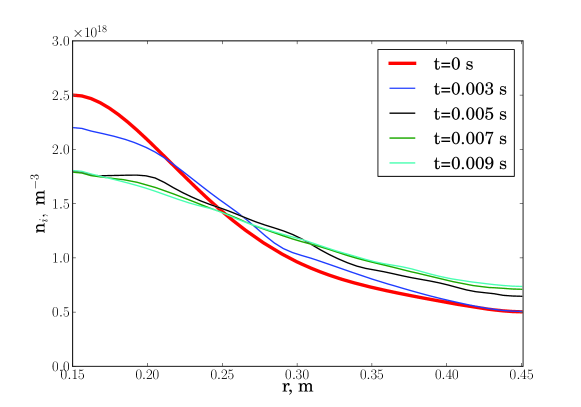
Figure 1: (Color Online) Relaxation of the density profile in a simulation without sources.

For the purposes of considering algorithms for average profile control in BOUT, it is convenient to represent the fluctuating variables at any spatial location as a sum of the time-average and perturbation,

$$f(\boldsymbol{{\rm x}},t)=\bar{f}(\boldsymbol{{\rm x}})+\tilde{f}(\boldsymbol{{\rm x}},t),$$ (5)

For cylindrically symmetric configuration it is also useful to separate $f$ into azimuthally symmetric and asymmetric components,

$$f(\boldsymbol{{\rm x}},t)=\left<{f(\boldsymbol{{\rm x}},t)}\right>+\{f(\boldsymbol{{\rm x}},t)\},$$ (6)

where $\left<{f}\right>=(1/2\pi)\int fd\theta$ and $\{f\}=f-\left<{f}\right>$ is the residual. Based on the ergodic hypothesis, it is assumed that the time-average $\bar{f}$ is equal to the azimuthal-average $\left<{f}\right>$, and statistical moments of $\tilde{f}$ and $\{f\}$ are equal. This separation of variables into an axisymmetric and non-axisymmetric part does not preclude a full nonlinear solution in BOUT, but it allows easier control over the average profiles of density, temperature and other quantities.

III.2 Profile maintenance: suppressing the azimuthal average

Following self-consistent time evolution of turbulence and macroscopic transport may be difficult because the time-scale separation can make such calculations too large to be practical. Additionally, including first-principles-based source terms, e.g., for density and temperature, can be complicated, involving models for the plasma source, atomic physics, radiation transport, etc.

Without attempting a self-consistent time evolution of turbulence and macroscopic transport one can consider intermediate time-scales $\tau\ll t\ll T$, where the macroscopic profiles can be taken as “frozen”, based on known measured experimental average profiles. In this case the time-evolution of only the non-axisymmetric part is considered, and a simple technique of maintaining the desired average profile is filtering out the axisymmetric part of evolving fields. This is illustrated in Fig. (2-3) showing the general appearance of $\phi$, $\delta n_{i}$, and the evolution of the density and potential fluctuation RMS in a simulation with “frozen” density profile. In Fig. (3), the potential is split into the turbulence-generated axisymmetric component $\left<\phi\right>$, and the non-axisymmetric residual $\{\phi\}=\phi-\left<\phi\right>$. One can observe the development of a zonal flow component $\left<{\phi(r)}\right>$ corresponding to sheared azimuthal flow.

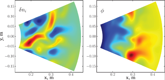
Figure 2: (Color Online) Spatial structure of the perturbed density (left) and turbulence-generated potential (right) at $t=5.2{\rm~{}ms}$.

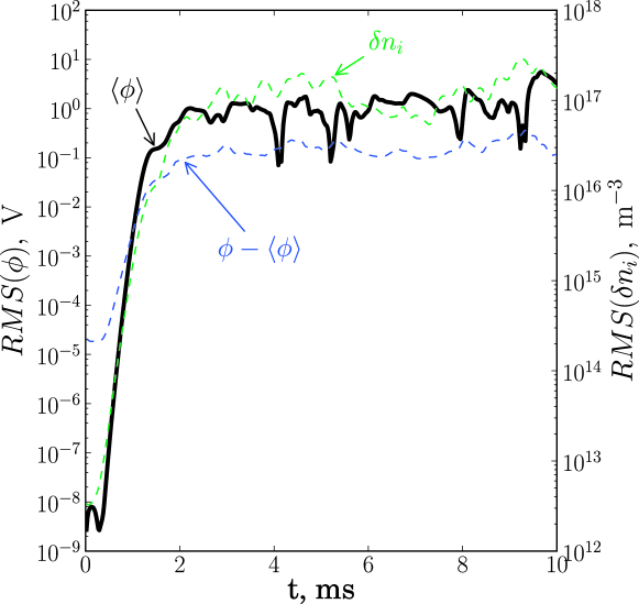
Figure 3: (Color Online) Time evolution of the density and potential fluctuation RMS in a typical simulation. The potential is split into the axisymmetric ($\left<\phi\right>$, zonal flow component) and the non-axisymmentric ($\phi-\left<\phi\right>$) components.

The easiest way to control the average profile is to suppress the evolution of the axisymmetric component by subtracting the azimuthal average of the right-hand side of Eqs. (1-3); for example, for the density:

$$\partial_{t}N=RHS-\left<{RHS}\right>_{\theta}$$ (7)

This is effectively introducing a time-dependent source/sink function necessary to maintain exactly the target density profile.

However, suppressing the axisymmetric part of fluctuations may interfere too much with the solution, and one can consider doing this not in the full domain but only on the boundary. This would constrain the boundary values, and may be enough to maintain the average profile close to the desired.

III.3 Profile maintenance through adding sources

A more physical method to control the profile is to use a source/sink term $S(r)$ designed in such a way that the average profile is maintained close to the experimentally measured profile. Rather than developing this source from first principles, an ad hoc source/sink is chosen in order to achieve the desired steady state profile in the simulation. As a first step, a simulation is performed using the method of subtracting out the azimuthal average to maintain the $\left<{N_{i}}\right>$ profile close to the “target” density profile ${N_{i0}(r)}$, which is based on a representative experimental probe measurements in LAPD. Once a steady-state turbulence solution is obtained, the radial particle flux is calculated from fluctuating density and potential,

$$\Gamma=\left<{N_{i}V_{Er}}\right>$$ (8)

Next, the effective volumetric density source $S(r)$ is calculated as

$$S=\nabla\cdot\Gamma$$ (9)

that can now be added to the density evolution equation, Eq. (1):

$$\partial_{t}N=RHS+S(r)$$ (10)

A subsequent simulation is run with this new source term and without suppressing the azimuthal average, allowing turbulent transport to compete with the source term. If needed, another iteration can be made by adjusting the source term to account for the mismatch between the BOUT predicted profile and the target. A more comprehensive approach to self-consistent time-evolution of turbulence and average profiles can be based on adding an adaptive source Dudson2009 ; however it is beyond the scope of this paper. In the present study extra iterations were not necessary; a single step was enough to produce stationary turbulence with average density profile close to the target profile, as shown in Fig. 4. The evolution of the density and potential in a typical BOUT simulation with density source and fixed values of the density at the radial boundary is presented in Fig. 5 (animation online).

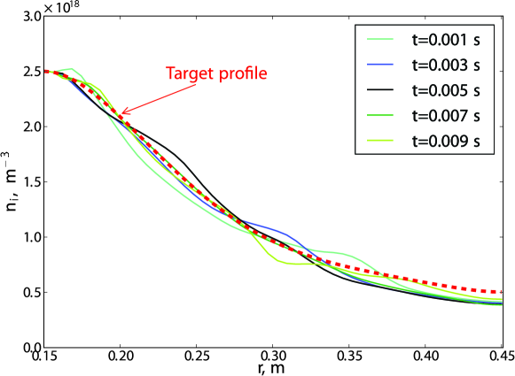
Figure 4: (Color Online) Instantaneous density profile $\left<{N_{i}}\right>$ in simulation with density source $S(r)$.

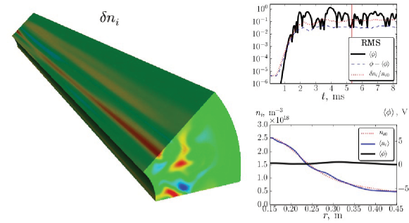
Figure 5: (Color Online) Evolution of density and potential in BOUT simulation with density source. Left: density fluctuations; right: RMS of the density perturbations and the axisymmetric and non-axisymmetric components of self-generated potential (top); average radial profiles of density and potential (bottom) (enhanced online).[URL: http://dx.doi.org/10.1063/1.3527987.1]

IV Comparison with LAPD data

Before any attempt is made to construct a full simulation of LAPD that self-consistently incorporates transport, first principles sources/sinks and profile evolution, it is necessary to ensure that the basic characteristics of the turbulence are correctly captured by the physical model being used. Initial simulations have been done using periodic axial boundary conditions and using the experimentally measured density profile. A constant temperature profile (5 eV) is used and the potential is allowed to evolve self-consistently (potential and flow profiles are not matched to experimentally measured profiles). The main experimental dataset used in this work is taken from Carter et al.. carter2009 , and includes measurements of plasma and turbulence profiles and two-dimensional correlation functions. Density fluctuations in BOUT are compared against ion saturation current $I_{i,sat}$ fluctuations measured in the experiment (making the currently unverified assumption that temperature fluctuations are negligible).

To be able to compare turbulence characteristics to the measured data for the experimentally relevant plasma parameters, the average profiles have to be maintained close to the experimental values during the simulation. To do so, the two methods described in section III are applied, either subtracting the azimuthal average of the right-hand side of the density equation, or adding a time-independent source function $S(r)$ to the right-hand side of Eq. (1).

Using these two methods, a steady-state turbulence for LAPD parameters is simulated, solving Eqs. (1-4) with the average density close to the experimental profile, for a range of ion-neutral collisionalities ($\nu_{in}/\Omega_{ci}=2\times 10^{-4},1\times 10^{-3},2\times 10^{-3}$). The estimated value for LAPD, based on neutral density $n_{n}\sim 5\times 10^{11}cm^{-3}$, is $\nu_{in}/\Omega_{ci}=2\times 10^{-3}$. The simulations are performed in the radial interval $0.15\leq r\leq 0.45{\rm~{}m}$, in an azimuthal segment of a cylinder of $\pi/4$ angle, assuming periodicity in the azimuthal angle and parallel direction. The grid size is $50\times 32\times 32$ points for radial, azimuthal and parallel coordinates. In order to improve the statistics, a series of uncorrelated runs is made with slightly different initial perturbations. In the experiment, a slow evolution of the mean density is observed on a $\sim 1-2\rm{~{}ms}$ time scale. BOUT simulations with fixed background profile can not capture the slow variation of the average density because the azumuthally symmetric component of density perturbation is continuously removed in BOUT simulation to maintain a constant profile. For the purposes of direct comparisons between BOUT results and the measured data, this slow evolution is removed from the experimental data by applying a temporal smoothing of the signal, which cuts off all frequencies below 800 Hz. For consistency, the same smoothing is applied to BOUT data.

IV.1 Fluctuations: temporal and spatial characteristics, PDF

The analysis of BOUT results shows that the $I_{i,sat}$ fluctuation amplitudes in LAPD data and the simulations have similar radial location near the cathode edge ($r\sim 28~{}\rm cm$), where the background density gradient is largest, as shown in Fig. 6. The absolute values of the fluctuations are of the same order of magnitude, with simulated amplitudes smaller by a factor $\lesssim$2 than the experimental data.

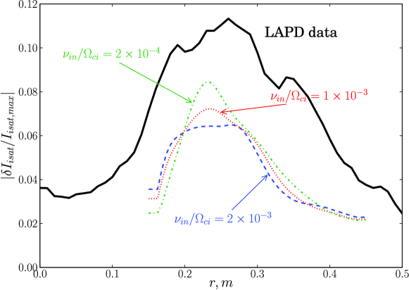
Figure 6: (Color Online) Radial distribution of the average ion saturation current fluctuations normalized to the maximum equilibrium profile value.

The comparison of the frequency power spectrum of the density fluctuations $\delta n/n$ to the LAPD measured spectrum is presented in Fig. 7. The spectra are integrated over the volume $0.22\leq r\leq 0.28~{}{\rm m}$, using a sliding Hanning window for averaging between the different simulation runs. Note that the total power in each spectrum is normalized to obtain the best fit to the experimental data. The power spectral shape from the BOUT simulation (for a range of $\nu_{in}$ values) is in a relatively good agreement with the measured spectrum (Fig. 7, b,d,e). At higher frequencies, $\gtrsim 10{\rm~{}kHz}$, the simulated spectra fall off faster than the measured spectrum. More studies are required to analyse the effect of additional features of the physical model (temperature profile and perturbations, sheath boundary conditions, etc.) on the power spectrum, as well as the numerical resolution. High frequencies corresponding to smaller spatial structures are potentially more affected by finite resolution effects. As a check of numerical convergence in terms of box size, the spectrum for $\nu_{in}/\Omega_{ci}={2}\times 10^{-3}$ is calculated with four times the size of the azimuthal extent of the grid and the number of azimuthal grid points ($N_{z}=128$). The spectrum shape is similar to the original calculation, with a smaller grid size (Fig. 7, b and c). These simulations were performed without the explicit ion viscosity term in the vorticity equation (3), therefore the only viscosity is due to the numerical discretization. Inclusion of the ion-ion viscosity term as discussed in the Appendix B corresponding to the ion temperature $T_{i}=0.1\rm eV$ does not significantly change the spectrum shape. The effects of viscosity in BOUT simulations is a subject of ongoing work. It is interesting to note that both the experimental and the simulation spectra exhibit an exponential power spectrum at higher frequencies (straight line on the log-lin plot), which is consistent with the presence of coherent structures pace2008 .

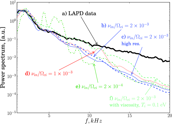
Figure 7: (Color Online) Frequency power spectrum of the density fluctuations: LAPD measurements (a) and BOUT simulations (b-f) for b) $\nu_{in}/\Omega_{ci}=2\times 10^{-3}$, c) $\nu_{in}/\Omega_{ci}=2\times 10^{-3}$ with $N_{z}=128$ azimuthal grid size, d) $\nu_{in}/\Omega_{ci}=1\times 10^{-3}$, e) $\nu_{in}/\Omega_{ci}=2\times 10^{-4}$, f) $\nu_{in}/\Omega_{ci}=2\times 10^{-3}$ with ion viscosity at $T_{i}=0.1{\rm~{}eV}$. Experimental density profile, $T_{e}=5eV$.

Another important characteristic of the turbulence is the probability distribution function (PDF) of fluctuation amplitudes. The PDF of $\delta n/RMS(\delta n)$ fluctuations from LAPD probe data is integrated over a volume of plasma $0.22\leq r\leq 0.28~{}{\rm m}$ and compared with the PDF from BOUT simulations in the same volume (Fig. 8). There are no normalizations or fit factors involved in this comparison. The experimental and the simulated PDFs are similar, with the average relative fluctuation $\left<{|\delta n/n|}\right>$ of 0.16 for the measured data and 0.09, 0.09, 0.08 for BOUT simulations with $\nu_{in}/\Omega_{ci}={2}\times 10^{-4},{1}\times 10^{-3},{2}\times 10^{-3}$. The PDF for $\nu_{in}/\Omega_{ci}={2}\times 10^{-3}$ case is the closest to the experimental data, which is consistent with the estimate of the neutral density in LAPD. Note that the distribution is mostly symmetric here because it is integrated over a radial inteval where the skewness is relatively low (Fig. 9).

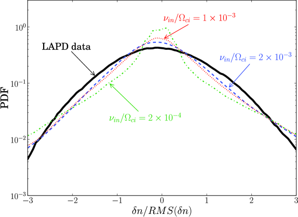
Figure 8: (Color Online) Probability distribution function of $\delta n/RMS(\delta n)$ fluctuation amplitude in BOUT simulations and LAPD data. PDF is volume averaged in the interval $0.22\leq r\leq 0.28{\rm~{}m}$.

Intermittent turbulence is observed in the edge plasmas of many experimental devices. This intermittency is usually attributed to generation and transport of coherent filaments of plasma, “blobs” or “holes” Carter2006 . One signature of the presence of these structures is the non-zero skewness of the density fluctuation PDF. Typically, positive skewness associated with convective transport of “blobs” is observed in LAPD measurements in the region outside of the cathode edge ($r\gtrsim 28~{}\rm cm$). Smaller negative values, associated with the “holes” are usually observed inside the cathode radius. The radial profile of the skewness of $\delta n$ is shown in Fig. 9. Except for the edge of the simulation domain which is affected by the imposed boundary conditions, the trend of the skewness profile, as well as the absolute values, is similar in BOUT simulations and in the LAPD data.

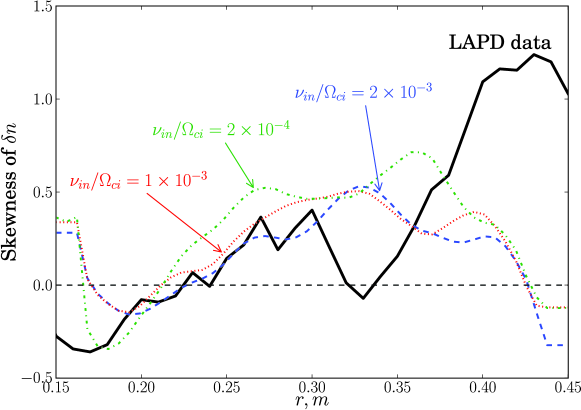
Figure 9: (Color Online) Skewness of $\delta n$ distribution in BOUT simulations and LAPD measurements.

Two-dimensional turbulent correlation functions are measured in LAPD using two probes: a fixed reference probe and a second probe that is moved shot-to-shot to many ($\sim$ 1000) spatial locations in a 2D plane perpendicular to the magnetic field. The reference probe remains at a fixed position that is close enough to the moving probe in the axial direction so that the parallel variation of the turbulent structures can be neglected. This allows to obtain the 2D spatial correlation function in the azimuthal plane. A similar “synthetic” diagnostic to post-process BOUT simulation results is constructed by calculating the correlations between a reference location and all other points in each azimuthal plane. The correlation length in BOUT simulation is of the same order, but larger than the measured value (Fig. 10).

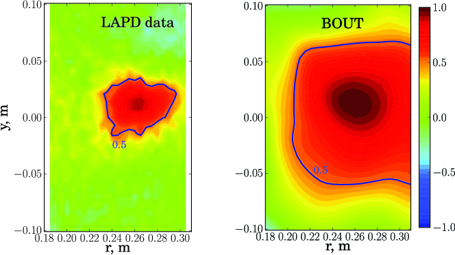
Figure 10: (Color Online) Correlation function for $I_{i,sat}$ fluctuations measured using a moving probe.

IV.2 Fluxes and sources vs. inferred source/sink in LAPD

An inferred particle source is required to maintain the density profile close to the experimental values, as described in section III.3. In BOUT simulations, the calculated source function $S(r)$ that produces steady-state turbulence with the desired density profile appears to be positive inside $r_{0}\sim 28~{}\rm cm$, and negative outside (Fig. (11)). Remarkably, the qualitative form and magnitude of the $S(r)$ profile is consistent with the assumption that within $\sim r_{0}$ there is an ionization source, and outside of $\sim r_{0}$ there is a sink due to parallel streaming to the end walls. In LAPD, the field lines inside $r\sim 28$ cm connect to the cathode that produces the primary ionizing electron beam. The magnitude of the inferred source is close to the estimated ionization source and parallel losses sink for LAPD plasma, $S_{source}\sim n_{n}n_{e}<\sigma v>_{i}\sim{2}\times 10^{20}~{}{\rm m}^{-3}/s$ and $S_{sink}\sim n_{i}C_{s}/L_{\parallel}\sim{5}\times 10^{20}~{}{\rm m}^{-3}/s$.

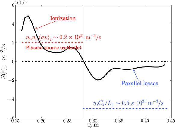
Figure 11: (Color Online) Inferred particle source required to maintain the measured density profile.

V Discussion

V.1 Plasma transport

One can calculate the effective diffusion coefficient by dividing the radial flux by the gradient of the equilibrium density,

$$D_{eff}=-\frac{\Gamma}{\nabla N_{i0}}$$ (11)

The turbulence-driven radial particle flux in BOUT simulations peaks near the maximum density profile gradient and is close to diffusive model value, with the effective diffusion coefficient $D_{eff}\sim 3{\rm~{}m^{2}/s}$ on the order of Bohm value, $D_{Bohm}\sim 8{\rm~{}m^{2}/s}$. The profiles of the average radial flux measured in LAPD and calculated in BOUT are shown in Fig. (12). The simulated flux is significantly lower than the measured flux in LAPD, but this difference is consistent with the difference in fluctuation amplitude shown in Fig. 6. It should also be noted that the measured flux profile is valid only for $r>28$cm as the measurement of azimuthal electric field fluctuations in LAPD is affected by fast electrons generated by the plasma source carter2009 .

While comparisons are made here to a diffusive model and particle transport in LAPD has been shown to be well modeled by Bohm diffusion maggs2007 , the simulated plasma turbulence has features that are usually associated with intermittency, as discussed in section IV.1: non-Gaussian fluctuations, as seen by non-zero standard statistical moments. The role of coherent structures and convective transport in BOUT simulations is the subject of ongoing investigation.

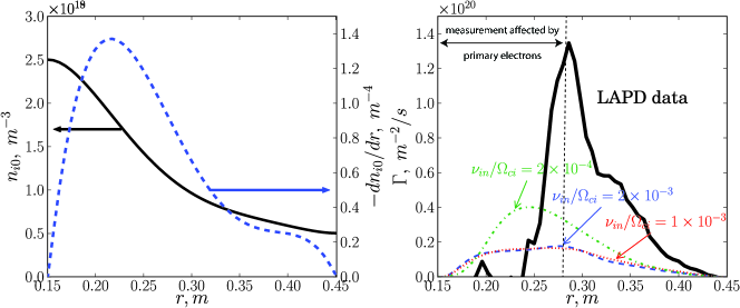
Figure 12: (Color Online) Left: Radial profiles of average $n_{i}$ and $dn_{i}/dr$. Right: radial particle flux $\Gamma$ from the measured LAPD data and BOUT simulations.

V.2 Numerical diagnostics and $\left<{E_{r}}\right>$ equation

An important part of the simulation effort is the framework for various diagnostics of the numerical solution. An obvious test of the solution is the check of the conservation laws (particle number, momentum, etc). However, depending on the choice of the radial boundary conditions and the form of the sources, the total number of particles, for example, is not necessarily conserved during the simulation. A more appropriate diagnostics in this case is the local check of the balance of the terms in each of the time evolution equations (1-3), at each point in space and time. As well as ensuring that the solution is correct, calculation of this balance also provides a useful insight into the relative importance of the physical terms.

This test can be done directly, using the explicit form of the equations (1-3) as they appear in the code, or indirectly, by calculating the conservation of physical quantities not directly solved for by BOUT. For the direct tests, the balance of the terms in BOUT equations is satisfied to the machine accuracy when the appropriate finite difference schemes are used in the diagnostic module.

Tests involving equations not directly solved by BOUT can be more subtle. An example is the equation for the azimuthal momentum. BOUT simulations in LAPD geometry show generation of self-consistent axisymmetric component of the potential. The dynamics of this zonal flow component can be derived from the vorticity equation as shown in Appendix A:

$$\partial_{t}\left<{NV_{\theta}}\right>=\left<{\varpi V_{r}}\right>+\frac{1}{r}\left<{N\partial_{\theta}\frac{\nabla_{\perp}\phi^{2}}{2}}\right>-\nu_{in}\left<{NV_{\theta}}\right>-\mu\partial_{r}\left<{\varpi}\right>$$ (12)

This expression is similar to the equation for the zonal flow component of the radial electric field that can be derived directly from the azimuthal projection of the ion momentum equation Tynan2006 :

$$\partial_{t}\left<{V_{\theta}}\right>=-\frac{1}{r^{2}}\partial_{r}\left(r^{2}\left<{V_{r}V_{\theta}}\right>\right)-\nu_{in}\left<{V_{\theta}}\right>+\mu\left(\partial_{r}^{2}\left<{V_{\theta}}\right>+\frac{1}{r}\partial_{r}\left<{V_{\theta}}\right>-\frac{1}{r^{2}}\left<{V_{\theta}}\right>\right)$$ (13)

The first term in the right-hand side of Eq. (12) and Eq. (13) is the turbulent Reynolds stress. If a stationary turbulent state exists, the time average of the Reynolds stress, which is the driving term for the zonal flows, is balanced by the ion-neutral collisions and the ion viscosity terms. This equation is not derived directly from the vorticity equation, therefore BOUT solution satisfies it only to the extent that the underlying assumptions in the derivation of the vorticity equation (3) are fulfilled.

Applying this diagnostic to BOUT output, it is found that the balance is well satisfied (within $\sim 5\%$) for Eq. (12) (with a small correction due to the linearization used in the inversion of Eq. (4)) and Eq. (13) with a particular choice of the finite difference scheme in the advection operators – the fourth order central scheme. However, for the first order upwind scheme used in most of nonlinear simulations presented here, the balance is not sufficiently well satisfied, which indicates that a higher numerical resolution is required to reach convergence for this diagnostic measure.

At present, a quantitative match between the average $\left<{E_{r}}\right>$ in the code and in the experimental data has not been obtained. However, at present the model does not include all physics (e.g., sheath, biasing, temperature perturbations) that is certainly important for setting the average radial electric field. Improving the model by adding to it the missing physics to address matching of $\left<{E_{r}}\right>$ is the subject of ongoing research.

V.3 Future work

A detailed verification study of linear instabilities in LAPD using BOUT Popovich2010a combined with a good qualitative and even partially quantivative agreement between nonlinear BOUT simulations and LAPD measuments presented here provides confidence in the relevance of these simulations to LAPD. It is, however, not a fully consistent first-principle model at present, and some potentially important physics is yet to be included. Most importantly, the experimentally measured temperature and flow profiles need to be matched and an evolution equation for temperature fluctuations, already implemented in BOUT, could be employed. The addition of a temperature gradient to the simulation would likely increase instability drive and result in a larger saturated turbulent amplitude and particle flux, more consistent with observation. Another significant improvement of the model that remains to be implemented is the sheath boundary condition at the end plates in the parallel direction. The axial boundary conditions are expected to be important in the formation of the radial electric field profile in LAPD, and a more physical description might help to understand and model the dynamics of the azimuthal flows and experimentally relevant potential profiles. The role of the ion viscosity on these flows is also a subject of ongoing work and has to be investigated in more detail. Additionally, including sheath boundary conditions along with temperature gradients, electron temperature fluctuations and an equation for temperature evolution can give rise to modifications to drift instabilities and introduce new modes, such as entropy waves Tsai1970 ; ricci2006 and conducting wall modes Berk1991 .

Although the linear calculations indicate that electromagnetic effects do not significantly affect drift wave instability in LAPD, magnetic field perturbations are required for Alfvén wave studies. Alfvén waves represent an important part of LAPD research, and nonlinear simulations of Alfvén waves using BOUT can contribute to the understanding of electromagnetic turbulence in LAPD.

VI Conclusions

A numerical 3-D model of plasma turbulence is applied to LAPD. The physics model includes equations for plasma density, electron parallel momentum, and current continuity, for partially ionized plasma. The model is implemented in the numerical code BOUT that is adapted for cylindrical geometry. This model has previously been successfully verified for a range of linear instabilities in LAPD Popovich2010a .

Two different methods for average profile control are applied in the simulations presented in this study. One approach consists of suppressing the azimuthal average of the density fluctuations by directly subtracting it from the time evolution equation. The second method uses a source/sink radial function that is constructed to balance steady-state radial transport flows. Both methods successfully maintain the average density profile close to the experimental value, required for comparisons with the measured turbulence characteristics.

Nonlinear BOUT simulations demonstrate a self-consistent evolution of turbulence and self-generated electric field and zonal flows, that saturates and results in a steady turbulent state. The simulated fluctuation amplitudes in the steady state are within a factor of 2 of the measured data, with a similar radial location near the cathode edge. The probability distribution function of the fluctuation amplitudes is comparable to the experimental distribution. Statistical properties of edge turbulence, such as the skewness, are often used as indication of the turbulence intermittency zweben2007 . In tokamak edge, the skewness is positive in the SOL (i.e. dominated by large amplitude events), but is sometimes negative inside the separatrix or limiter radius (i.e. with density “holes”), e.g. seen in DIII-D Boedo2003 and NSTX Boedo2001 . This feature is similar to LAPD data, and reproduced in BOUT simulations. Despite the intermittent character of turbulence, as indicated by non-Gaussian PDF, the turbulent particle flux magnitude is consistent with diffusive model with diffusion coefficient on the order of $D_{Bohm}$. The inferred particle source/sink function required to maintain the simulated steady-state density profile close to experimental value is consistent with the estimates of ionization sources and parallel losses in LAPD discharge.

The spatial and temporal structures of the fluctuations are consistent with the LAPD measurements, however the correlation length in BOUT simulations is larger than in the experiment.

Although some elements of the physical model still remain to be implemented (sheath parallel boundary conditions, azimuthal flow matching, electron temperature fluctuations, etc.), the agreement between certain features of the experimental data and simulations based on this relatively simple model lends confidence in the applicability of these simulations to the LAPD plasmas.

Appendix A Azimuthal momentum equation

The equation describing the evolution of the surface-averaged azimuthal momentum can be derived from the vorticity equation:

$$\partial_{t}\varpi=-\boldsymbol{{\rm v}_{E}}\cdot\nabla\varpi-\nabla_{\parallel}(Nv_{\parallel})+\boldsymbol{{\rm b}}\times\nabla N\cdot\nabla\boldsymbol{{\rm v}_{E}}^{2}/2-\nu_{in}\varpi+\mu_{i}\nabla_{\perp}^{2}\varpi$$ (14)

where the potential vorticity is

$$\varpi=\nabla_{\perp}\cdot\left(N\nabla_{\perp}\phi\right)$$ (15)

Define surface and volume averaging by

$$\left<{f(r,\theta,z)}\right>=\frac{1}{2\pi L}\int_{0}^{2\pi}\int_{0}^{L}{fdzd\theta}$$ (16)

$$\left<{f(r,\theta,z)}\right>_{V}=\frac{1}{V}\int_{r_{a}}^{r}{\left<{f(r^{\prime},\theta,z)}\right>r^{\prime}dr^{\prime}}$$ (17)

Note the identity

$$\left<{\nabla_{\perp}^{2}f}\right>=\nabla_{\perp}^{2}\left<{f}\right>$$ (18)

For LAPD geometry, the convention is $B_{z}=-B_{p}$, so $\boldsymbol{{\rm b}_{0}}=-\boldsymbol{{\rm z}}$. In normalized variables, $\boldsymbol{{\rm v}_{E}}=\boldsymbol{{\rm b}_{0}}\times\nabla\phi$:

$$V_{r}=-b_{z}\frac{1}{r}\frac{\partial\phi}{\partial\theta}=\frac{1}{r}\frac{\partial\phi}{\partial\theta}$$

$$V_{\theta}=b_{z}\frac{\partial\phi}{\partial r}=-\frac{\partial\phi}{\partial r}$$

The equation for the evolution of the azimuthal flows can be obtained from the vorticity equation (14) by volume averaging. Applying Gauss theorem and assuming that the boundary conditions on the internal boundary are such that all surface integrals over the internal surface $r=r_{a}$ vanish, the following expression for the volume-average of the vorticity is obtained:

$$\left<{\varpi}\right>_{V}=\frac{2\pi L}{V}\left<{N\partial_{r}\phi}\right>=-\frac{2\pi L}{V}\left<{NV_{\theta}}\right>$$ (20)

The ion-ion viscosity term:

$$\left<{\nabla_{\perp}^{2}\varpi}\right>_{V}=\frac{2\pi L}{V}\left<{\partial_{r}\varpi}\right>=\frac{2\pi L}{V}\partial_{r}\left<{\varpi}\right>$$ (21)

The advection term can be rewritten as:

$$\left<{\boldsymbol{{\rm v}_{E}}\cdot\nabla\varpi}\right>_{V}=\left<{\nabla\cdot\left(\varpi\boldsymbol{{\rm v}_{E}}\right)-\varpi\nabla\cdot{\boldsymbol{{\rm v}_{E}}}}\right>_{V}$$ (22)

where in straight field the last term vanishes. Applying Gauss theorem, the full divergence becomes a surface average:

$$\left<{\nabla\cdot\left(\varpi\boldsymbol{{\rm v}_{E}}\right)}\right>_{V}=\frac{2\pi L}{V}\left<{\varpi V_{r}}\right>$$ (23)

The fourth term in Eq. (14) can be written as a full divergence:

$$\boldsymbol{{\rm b}}\times\nabla N\cdot\nabla\frac{\boldsymbol{{\rm v}_{E}}^{2}}{2}=\nabla\cdot\left(\frac{\boldsymbol{{\rm v}_{E}}^{2}}{2}\boldsymbol{{\rm b}}\times\nabla N\right)-\frac{\boldsymbol{{\rm v}_{E}}^{2}}{2}\nabla\cdot\left(\boldsymbol{{\rm b}}\times\nabla N\right)=\nabla\cdot\left(\frac{\nabla_{\perp}\phi^{2}}{2}\boldsymbol{{\rm b}}\times\nabla N\right)$$ (24)

The volume integral is then transformed info surface average

$$\left<{\boldsymbol{{\rm b}}\times\nabla N\cdot\nabla\frac{\boldsymbol{{\rm v}_{E}}^{2}}{2}}\right>_{V} = \frac{2\pi L}{V}\left<{\frac{\nabla_{\perp}\phi^{2}}{2}\boldsymbol{{\rm b}}\times\nabla N\cdot\hat{r}}\right>$$

$$= \frac{2\pi L}{V}\frac{1}{r}\left<{\frac{\nabla_{\perp}\phi^{2}}{2}\partial_{\theta}N}\right>=-\frac{2\pi L}{V}\frac{1}{r}\left<{N\partial_{\theta}\frac{\nabla_{\perp}\phi^{2}}{2}}\right>$$

Collecting all terms, one obtains the surface-averaged azimuthal momentum evolution equation:

$$\partial_{t}\left<{NV_{\theta}}\right>=\left<{\varpi V_{r}}\right>+\frac{1}{r}\left<{N\partial_{\theta}\frac{\nabla_{\perp}\phi^{2}}{2}}\right>-\nu_{in}\left<{NV_{\theta}}\right>-\mu\partial_{r}\left<{\varpi}\right>$$ (26)

Appendix B Ion viscosity

Including the ion-ion viscosity effects results in an additional term in the vorticity equation (3). Viscous force $\nabla\cdot\Pi$ (where $\Pi$ is the stress tensor $\boldsymbol{{\rm v}}\boldsymbol{{\rm v}}-v^{2}/3{\bf\hat{I}}$) in the ion motion equation induces a perpendicular drift $\boldsymbol{{\rm v}}_{i\perp\mu}=\boldsymbol{{\rm b}}\times\left(\nabla\cdot\Pi\right)$ to the lowest order, which translates into an additional perpendicular current component $\boldsymbol{{\rm j}}_{\perp,\mu}=en\boldsymbol{{\rm b}}\times\left(\nabla\cdot\Pi\right)$. To simplify the final form of the viscous term, it is assumed that density perturbations are small and the equilibrium gradients are negligible compared to the perturbed quantities. Then the extra term due to viscosity in the vorticity equation can be written as

$$\nabla\cdot j_{\perp,\mu}=en\nabla\cdot\left\{\boldsymbol{{\rm b}}\times\left(\nabla\cdot\Pi\right)\right\}=-en\boldsymbol{{\rm b}}\cdot\left\{\nabla\times\left(\nabla\cdot\Pi\right)\right\}$$ (27)

Using Braginskii expressions for the stress tensor Braginskii1965 with perpendicular ion velocity $\boldsymbol{{\rm v}}_{i\perp}=\boldsymbol{{\rm v}_{E}}=\boldsymbol{{\rm b}}\times\nabla\phi$ to the lowest order, it can be shown that the extra term in the vorticity equation (3) is $\mu_{i}\nabla_{\perp}^{2}\varpi$.

Depending on the ion magnetization, one should choose either the magnetized or unmagnetized viscosity expression for the coefficient $\mu_{i}$: $\mu_{i}=\eta_{1}^{i}=0.3nT_{i}/\Omega_{ci}^{2}\tau_{i}$ for $\Omega_{ci}\tau_{i}\gg 1$ or $\mu_{i}=\eta_{0}^{i}=0.96nT_{i}\tau_{i}$ for $\Omega_{ci}\tau_{i}\ll 1$. The estimate of the ion magnetization parameter $\Omega_{ci}\tau_{i}$ for typical LAPD values (${\rm He}^{4}$, $B_{0}=400~{}\rm G$, $n_{i}\sim{3}\times 10^{18}~{}{\rm m}^{-3}$, $T_{i}\sim 1~{}\rm eV$) is close to unity. The ion temperature in LAPD is not directly measured; the estimate from the electron-ion energy exchange and the parallel losses balance indicates that $T_{i}$ is in the range $0.1-1~{}\rm eV$. Preliminary BOUT simulations with ion viscosity are consistent with the experimental measurements for low ion temperatures, $T_{i}\sim 0.1~{}\rm eV$, which corresponds to unmagnetized ion regime.

Appendix C Discretization in the parallel coordinate

Consider the local drift mode dispersion relation for the simplest case, without electron inertia and electromagnetic terms, when it becomes a quadratic equation, as given in elementary plasma textbooks Chen1984 :

$$(\omega-1)i\sigma_{||}+\omega^{2}=0,$$ (28)

where

$$\sigma_{||}=\left(\frac{k_{||}}{k_{\perp}}\right)^{2}\frac{\Omega_{ci}\Omega_{ce}}{\nu_{ei}\omega_{*}},$$ (29)

$$\omega_{*}=k_{\perp}v_{pe}=\frac{k_{\perp}}{L_{n}}\frac{T_{e0}}{m_{i}\Omega_{ci}}$$ (30)

and $\omega$ is normalized to $\omega_{*}$.

Now consider the effect of finite-difference discretization on Eq. (28). For simplicity assume no radial structure so that the radial part of the solution can be dropped. There are just two coordinates then - the drift wave propagation direction $y$ and the parallel direction $z$.

Now let’s focus on the parallel discretization. Parallel derivatives that are represented by $ik_{||}$ in the Fourier form will become something different in the discretized equation, depending on the type of discretization. For example, applying the 2^nd central difference for a single mode $\exp(ik_{||}z)$ one obtains

$$\frac{df}{dz}\rightarrow\frac{\exp(ik_{||}z_{j+1})-\exp(ik_{||}z_{j-1})}{2h}=\frac{i\sin(k_{||}h)}{h}$$ (31)

Here $h$ is parallel grid spacing, $z_{j}$=$jh$.

One can notice that at large wavenumbers, $k\sim\pi/h$, the finite-difference representation is very poor. In this example, from Eq. 28, for ${\sigma_{||}}\gg$1 the growth rate scales as $\gamma\propto 1/k_{||}^{2}$, i.e., large $k_{||}$ should stabilize the modes. Conversely, in the discretized dispersion relation it will become $\gamma\propto 1/(\sin(k_{\parallel}h))^{2}$ which would become singular at the Nyquist wavenumber $k_{\parallel}=\pi/h$, which can be manifested in unphysical behavior of such modes. The possibility of unphysical behavior of high-k modes caused by spatial discretization, in particular the “red-black” numerical instability, is well-known in the CFD community, and historically the main remedy was using staggered grid Patankar1980 . A more recent popular method is discretization on collocated grids adding a dissipative biharmonic (i.e. 4^th derivative) term to suppress the “red-black” instability (e.g., the Rhie-Chow interpolation).

Consider the effects of staggered grid for the discretized drift mode dispersion relation. Assume that $N_{i}$, $\phi$, $\varpi$ are specified on one grid, and $j_{||}$, $V_{||e}$ are specified on another grid shifted by $h$/2. Then, $k_{||}^{2}$ in the dispersion relation (28) can be tracked down to the derivatives

$$\frac{\partial j_{||}}{\partial z}\rightarrow(j_{||,j}-j_{||,j-1})/h=\exp(-ikh/2)\frac{i\sin(kh/2)}{h/2}$$ (32)

and

$$\frac{\partial\phi_{||}}{\partial z}\rightarrow(\phi_{j+1}-\phi_{j})/h=\exp(ikh/2)\frac{i\sin(kh/2)}{h/2},$$ (33)

which combine to produce

$$k_{||}^{2}\rightarrow-\left(\frac{\sin(kh/2)}{h/2}\right)^{2}$$ (34)

One can note that Eq. (34) does not become zero for any mode supported by the grid, $-\pi/h\leq k\leq\pi/h$, which is an important improvement.

Since the staggered grid approach is more cumbersome for implementation, in particular for parallel computation, it is desirable to stay with collocated grids, if possible. In this example one can come up with discretization Eq. (32-33) on collocated grids by combining right-sided and left-sided 1^st order discretization. This method, which we call “quasi-staggered grid”, has been successfully applied in BOUT to eliminate spurious modes due to parallel discretization.

References

- (1) A. Schekochihin and S. Cowley, Phys. Plasmas 13, 056501 (2006).
- (2) E. Quataert, W. Dorland, and G. W. Hammett, ApJ 577, 524 (2002).
- (3) H. Hasegawa, M. Fujimoto, T. D.Phan, H. Reme, A. Balogh, M. W. Dunlop, C. Hashimoto, and R. TanDokoro, Nature 430, 755 (2004).
- (4) G. Tynan, A. Fujisawa, and G. McKee, Plasma Phys. Control. Fusion 51, 113001 (2009).
- (5) J. Connor, Plasma Phys. Control. Fusion 37, A119 (1995).
- (6) W. Horton, Rev. Mod. Phys. 71, 735 (1999).
- (7) S. J. Zweben, J. A. Boedo, O. Grulke, C. Hidalgo, B. LaBombard, R. J. Maqueda, P. Scarin, and J. L. Terry, Plasma Phys. Control. Fusion 49, S1 (2007).
- (8) B. B. Kadomtsev, Plasma Turbulence, Academic Press, London, 1965.
- (9) L. Stenflo, J. Plasma Physics 4, 585 (1970).
- (10) S. C. Cowley, R. M. Kulsrud, and R. Sudan, Phys. Fluids B 3, 2767 (1991).
- (11) W. Dorland, F. Jenko, M. Kotschenreuther, and B. Rogers, Phys. Rev. Lett. 85, 5579 (2000).
- (12) P. S. Iroshnikov, AZh 40, 742 (1963).
- (13) R. H. Kraichnan, Phys. Fluids 8, 1385 (1965).
- (14) S.-I. Itoh and K. Itoh, Phys. Rev. Lett. 60, 2276 (1988).
- (15) K. C. Shaing and E. C. Crume, Phys. Rev. Lett. 63, 2369 (1989).
- (16) H. Biglari, P. H. Diamond, and P. W. Terry, Phys. Fluids B 2 (1990).
- (17) M. Greenwald, Phys. Plasmas 17, 058101 (2010).
- (18) P. W. Terry, M. Greenwald, J.-N. Leboeuf, G. R. McKee, D. R. Mikkelsen, W. M. Nevins, D. E. Newman, and D. P. Stotler, Phys. Plasmas 15, 062503 (2008).
- (19) W. Gekelman, H. Pfister, Z. Lucky, J. Bamber, D. Leneman, and J. Maggs, Rev. Sci. Inst. 62, 2875 (1991).
- (20) G. R. Tynan, M. J. Burin, C. Holland, G. Antar, and P. H. Diamond, Plasma Phys. Control. Fusion 46, A373 (2004).
- (21) C. M. Franck, O. Grulke, and T. Klinger, Phys. Plasmas 9, 3254 (2002).
- (22) S. Shinohara, Y. Miyauchi, and Y. Kawai, Plasma Phys. Control. Fusion 37, 1015 (1995).
- (23) A. G. Lynn, M. Gilmore, C. Watts, J. Herrea, R. Kelly, S. Will, S. Xie, L. Yan, and Y. Zhang, Rev. Sci. Inst. 80, 103501 (2009).
- (24) T. Pierre, G. Leclert, and F. Braun, Rev. Sci. Inst. 58, 6 (1987).
- (25) N. Kasuya, M. Yagi, M. Azumi, K. Itoh, and S.-I. Itoh, J. Phys. Soc. Japan 76, 044501 (2007).
- (26) C. Holland, G. R. Tynan, J. H. Yu, A. James, D. Nishijima, M. Shimada, and N. Taheri, Plasma Phys. Control. Fusion 49, A109 (2007).
- (27) V. Naulin, T. Windisch, and O. Grulke, Phys. Plasmas 4, 012307 (2008).
- (28) G. N. Kervalishvili, R. Kleiber, R. Schneider, B. D. Scott, O. Grulke, and T. Windisch, Contrib. Plasma Phys. 48, 32 (2008).
- (29) T. Windisch, O. Grulke, R. Schneider, and G. N. Kervalishvili, Contrib. Plasma Phys. 48, 58 (2008).
- (30) B. N. Rogers and P. Ricci, Phys. Rev. Lett. 104, 225002 (2010).
- (31) X. Q. Xu and R. H. Cohen, Contrib. Plasma Phys. 36, 158 (1998).
- (32) M. Umansky, X. Xu, B. Dudson, L. LoDestro, and J. Myra, Contrib. Plasma Phys. 180, 887 (2009).
- (33) P. Popovich, M. Umansky, T. A. Carter, and B. Friedman, Phys. Plasmas 17, 102107 (2010).
- (34) T. A. Carter and J. E. Maggs, Phys. Plasmas 16, 012304 (2009).
- (35) J. E. Maggs, T. A. Carter, and R. J. Taylor, Phys. Plasmas 14, 052507 (2007).
- (36) S. I. Braginskii, Transport processes in a plasma, in Reviews of Plasma Physics, edited by M. A. Leontovich, volume 1, pages 205–311, Consultants Bureau, New York, 1965.
- (37) S. Vincena, W. Gekelman, and J. E. Maggs, Phys. Plasmas 8, 3884 (2001).
- (38) J. E. Maggs and G. J. Morales, Phys. Plasmas 10, 2267 (2003).
- (39) J. R. Peñano, G. J. Morales, and J. E. Maggs, Phys. Plasmas 4, 555 (1997).
- (40) M. Ono and R. Kulsrud, Phys. Fluids 18, 1287 (1975).
- (41) B. Dudson, private communication, 2009.
- (42) D. Pace, M. Shi, J. Maggs, G. Morales, and T. Carter, Phys. Rev. Lett. 101, 085001 (2008).
- (43) T. A. Carter, Phys. Plasmas 13, 010701 (2006).
- (44) G. R. Tynan, C. Holland, J. H. Yu, A. James, D. Nishijima, M. Shimada, and N. Taheri, Plasma Phys. Control. Fusion 48, S51 (2006).
- (45) S.-T. Tsai, F. W. Perkins, and T. H. Stix, Phys. Fluids 13, 2108 (1970).
- (46) P. Ricci, B. N. Rogers, W. Dorland, and M. Barnes, Phys. Plasmas 13, 062102 (2006).
- (47) H. L. Berk, D. D. Ryutov, and Y. Tsidulko, Phys. Fluids B 3, 1346 (1991).
- (48) J. A. Boedo, D. L. Rudakov, R. A. Moyer, G. R. McKee, R. J. Colchin, M. J. Schaffer, P. G. Stangeby, W. P. West, S. L. Allen, T. E. Evans, R. J. Fonck, E. M. Hollmann, S. Krasheninnikov, A. W. Leonard, W. Nevins, M. A. Mahdavi, G. D. Porter, G. R. Tynan, D. G. Whyte, and X. Xu”, Phys. Plasmas 10, 1670 (2003).
- (49) J. A. Boedo, D. Rudakov, R. Moyer, S. Krasheninnikov, D. Whyte, G. McKee, G. Tynan, M. Schaffer, P. Stangeby, P. West, S. Allen, T. Evans, R. Fonck, E. Hollmann, A. Leonard, A. Mahdavi, G. Porter, M. Tillack, and G. Antar, Phys. Plasmas 8, 4826 (2001).
- (50) F. F. Chen, Introduction to Plasma Physics and Controlled Fusion, Plenum Press, New York, 1984.
- (51) S. V. Patankar, Numerical Heat Transfer and Fluid Flow, Hemisphere Publishing Corporation, New York, 1980.