Analyzing the Low State of EF Eridani with Hubble Space Telescope Ultraviolet Spectra

Abstract

Time-resolved spectra throughout the orbit of EF Eri during its low accretion state were obtained with the Solar Blind Channel on the Advanced Camera for Surveys onboard the Hubble Space Telescope. The overall spectral distribution exhibits peaks at 1500 and 1700Å, while the UV light curves display a quasi-sinusoidal modulation over the binary orbit. Models of white dwarfs with a hot spot and cyclotron emission were attempted to fit the spectral variations throughout the orbit. A non-magnetic white dwarf with a temperature of $\sim$10,000K and a hot spot with central temperature of 15,000K generally matches the broad absorptions at 1400 and 1600Å with those expected for the quasimolecular H features H₂ and H${}_{2}^{+}$. However, the flux in the core of the Ly$\alpha$ absorption does not go to zero, implying an additional component, and the flux variations throughout the orbit are not well matched at long wavelengths. Alternatively, a 9500K white dwarf with a 100 MG cyclotron component can fit the lowest (phase 0.0) fluxes, but the highest fluxes (phase 0.5) require an additional source of magnetic field or temperature. The 100 MG field required for the UV fit is much higher than that which fits the optical/IR wavelengths, which would support previous suggestions of a complex field structure in polars.

1 Introduction

EF Eri is a well-studied cataclysmic variable that contains a highly magnetic white dwarf. It was identified in 1979 as the fourth known Polar (Griffiths et al. 1979; Hiltner et al. 1979; Tapia 1979) with an 81 min orbital period. During the next 20 years, it remained in a bright high state near 14th mag, with highly modulated optical, IR and X-ray light curves due to a high mass transfer rate and X-ray and cyclotron emission from the accretion region (Bailey et al. 1982). Models of the cyclotron humps determined magnetic field strengths of 16.5 and 21 MG (Ferrario, Bailey & Wickramasinghe 1996). However, in 1997, EF Eri entered a low state near 18th mag (Wheatley & Ramsay 1998) which lasted for 9 years, with only short excursions to a high state since 2006. Low states are advantageous to study the underlying white dwarf and secondary star without the effects of the accretion flow. In the low state, the optical spectrum of EF Eri shows broad Balmer absorption lines with Zeeman splitting indicating a 14 MG field (Wheatley & Ramsay 1998). Beuermann et al. (2000) modeled the optical spectrum with a 9500K white dwarf and a 15,000K hot spot over 6% of its surface. As there were no features from a secondary star, they concluded that the spectral type of the companion must be later than M9. Spitzer mid-IR emission suggested the companion was an L or T dwarf (Howell et al. 2006b). Howell et al. (2006a) used the H$\alpha$ emission from this substellar secondary to produce a radial velocity curve, which provided a spectroscopic ephemeris as well as a mass estimate for the secondary of 0.055 M_⊙ for a white dwarf mass of 0.6 M_⊙. Thorstensen (2003) attempted parallax measurements but the faintness of the source and the assumptions used yielded a small range of distances centered near 113 pc or a larger range near 163 pc.

While the accretion rate in low states is reduced by several orders of magnitude from the high state, and there is no evidence of a stream of mass transfer during the low state of EF Eri, UV studies have shown that hot spots with temperatures of 30,000-70,000K are likely present on the white dwarfs of Polars during low states. IUE observations of AM Her in the low state revealed an orbital-phase dependent flux modulation, which Heise & Verbunt (1988) interpreted as the signature of moderate heating of a large fraction of the white dwarf surface. Gänsicke et al. (1995) developed this hypothesis further, showing that a large pole cap covering $\sim 10\%$ of the white dwarf surface is present both during the high state and the low state, and that, at least in the case of AM Her, the luminosity of this heated pole cap is comparable to that of the hard X-ray and cyclotron emission from the post-shock region, solving the so-called “soft X-ray puzzle”, i.e. the soft X-ray excess with respect to the simple reprocessing model of Lamb & Masters (1979) and King & Lasota (1979). Evidence for large, “warm” pole-caps was found in many other polars (e.g. Stockman et al. 1994; Gänsicke et al. 2000, Schwope et al. 2002, Araujo-Betancor et al 2005). Gänsicke et al (1998) developed a 3-dimensional model of a white dwarf with a heated pole cap to analyze high-time resolution HST/GHRS observations of AM Her in a high state, and FUSE and HST/STIS observations of AM Her in a low state (Gänsicke et al 2006), leading to more precise constraints on the size, temperature, and location of the heated pole cap. Especially for the low-state data, where no emission from the accretion stream was present, this model provided an excellent fit to both the observed modulation of the ultraviolet flux, as well as to the changes in the Lyman line profiles.

GALEX photometric observations of EF Eri during its low state (Szkody et al. 2006; 2008) in two broad band filters centered near 1550Å and 2300Å were modeled with a 9500K white dwarf and a spot of radius 5.5^∘ with a temperature of 24,000K. Schwope et al. (2007) analyzed archival XMM-Newton observations to detect an X-ray flux of 6$\times$10^-14 erg cm^-2 s^-1 during the low state, corresponding to an x-ray luminosity of 2$\times$10²⁹ erg s^-1. While the specific accretion rate would then be only 0.01 g cm^-2 s^-1, implying no accretion shock, they suggested the X-rays come from some residual accretion at the poles. Li et al. (1994, 1995) have produced models for high field white dwarfs where the white dwarf can capture all the stellar wind from the secondary and funnel it to the poles.

Further support for some accretion during the low state comes from the presence of cyclotron humps in the IR (Harrison et al. 2004; Campbell et al. 2008). Campbell et al. (2008) explored whether high magnetic field cyclotron emission could be producing the GALEX UV variations as well as the IR. The high field (240 MG) system AR UMa does show UV variability that is likely due to cyclotron emission (Gänsicke et al. 2001) and QS Tel showed humps at 2200Å and 2430Å that could be interpreted as cyclotron humps in a 65 MG field (Rosen et al. 2001). The models of Campbell et al. (2008) showed that the UV variations in EF Eri could be cyclotron if the field was 115 MG, while the IR variations require a field of 13 MG. Some confirmation of the high field required for the UV is evident from the work of Beuermann et al. (2007), who used Zeeman tomography and determined that EF Eri has a complex field with some regions as high as 100 MG.

In order to better understand the cause of the UV light and variability, we obtained time-resolved spectroscopy with the Hubble Space Telescope (HST). These data and our modeling efforts with a heated polecap and cyclotron emission are described below.

2 Observations

The Solar Blind Channel (SBC) on the Advanced Camera for Surveys (ACS) was used with prism PR110L throughout four sequential HST orbits on 2008 January 17. This prism provides wavelength coverage with useful sensitivity from $\sim$1200-1900Å, the prism results in non-linear resolution from $\sim$2Å pixel^-1 at the blue end to $\sim$40Å pixel^-1 at the red end. The ACCUM mode was used with continuous exposures of 239 sec during each satellite orbit. The first orbit had 9 exposures (due to the setup time) while the remaining 3 orbits contained 10 exposures. The setup exposure on the target was accomplised with the F140LP filter and an integration time of 15 s. The observation times for each orbit are summarized in Table 1.

The reduction package aXe1.6 (Kuemmel et al. 2009) provided by STScI was used to extract the target and produce a flux and wavlength calibrated spectrum for each 239 sec exposure. To obtain the best flux level, we used an extraction width of $\pm$17 pixels corresponding to $\pm$ 0.5 arcsec. To show the variability, we created light curves in six bands (1220-1260Å, 1330-1380Å, 1430-1530Å, 1530-1640Å, 1640-1720Å, and 1780-1820Å) by integrating the fluxes within these regions. Phases were calculated using the spectroscopic phasing of Howell et al. (2006a).

To insure that EF Eri was in its low state during the HST observations, we solicited optical ground data from AAVSO members and observatories in the Northern and Southern hemisphere in the nights preceding and following the HST times. The New Mexico State University (NMSU) 1m telescope provided three nights of measuremnts with UBVR filters and time-resolved differential light curves in V filter. The Small and Moderate Aperture Research Telescope System (SMARTS) obtained B band photometry with a CCD on the 0.9m telescope. Spectra throughout an orbit were obtained on the 3.5m telescope at Apache Point Observatory (APO) using the Dual Imaging Spectrograph (DIS) with the high resolution gratings (resolution $\sim$2Å) that provided simultaneous spectra from 3900-5100Å and from 6300Å to 7300Å. The times of the optical data close to the HST observation are listed in Table 1.

3 Optical Results

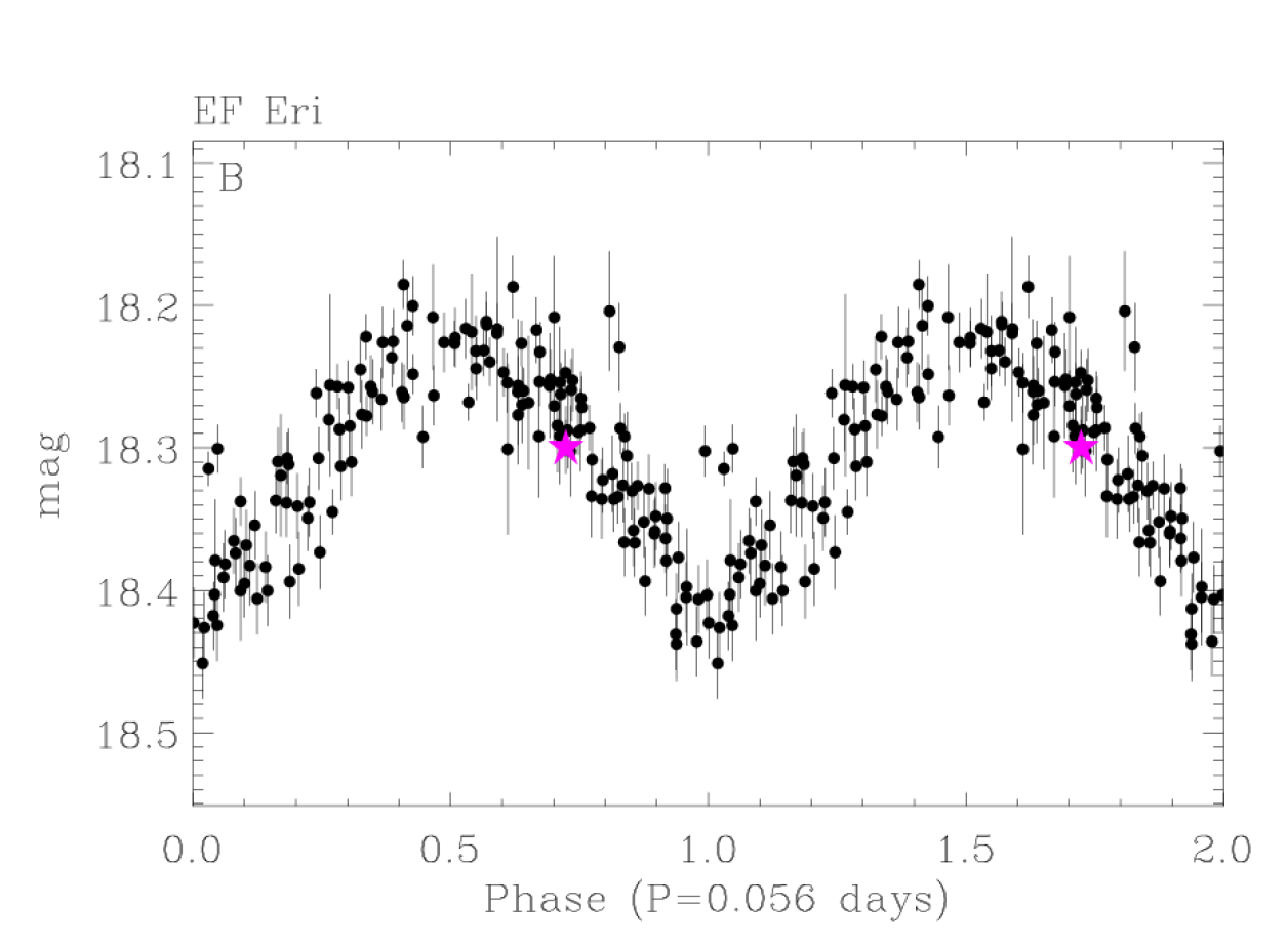
Figure 1: SMARTS composite $B$ data for the extended low state during which the HST observations were made. The light curve is comprised of 152 points on 68 nights from 2007 June 20 to 2008 Mar 23. The star near phase 0.7 is the night of 2008 Jan 16.

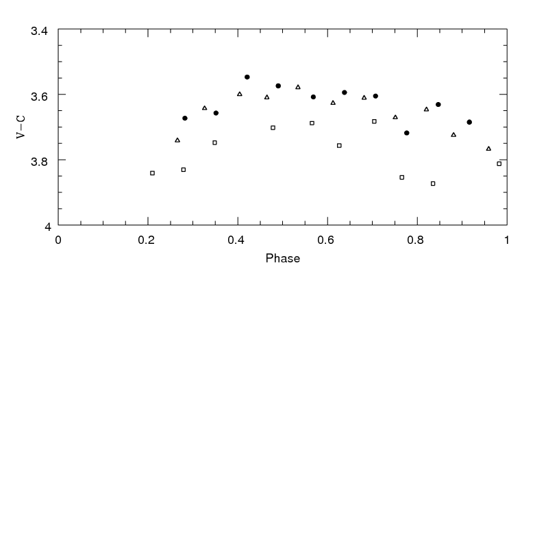
Figure 2: NMSU $V$ data relative to a comparison star for Jan 15 (dots), Jan 16 (triangles) and Jan 18 (squares). Error bars are $\pm$0.03-0.05 mag for Jan 15 and 16 and $\pm$0.06-0.08 mag on Jan 18.

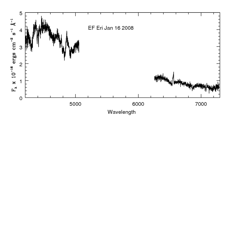
Figure 3: DIS blue and red spectra averaged over the orbit of EF Eri. The Balmer emission shows that some level of activity on the secondary star is present.

Both the optical photometry and spectroscopy showed that EF Eri remained in its deep and extended low state during the HST observations. The calibrated data provided B=18.29, V=18.40 and R=18.10 the night preceeding the HST observation. The SMARTS photometric point from that night is shown in Figure 1 as a star superposed on the B light curve accumulated on 68 nights from 2007 June 20 to 2008 March 23 while EF Eri was in a low state (Walter 2009). The NMSU V light curves from the nights preceding and following the HST times are shown in Figure 2. Both light curves show the normal low state optical modulation with a steeper rise to a peak brightness near phase 0.5 and a slower decline to minimum near phase 0.0. While the data from January 18th show EF Eri slightly fainter, the larger error bars on this night are within the range of variation evident in Figure 1. The APO spectra (Figure 3) show the typical low state features of broad Balmer absorption lines from the white dwarf flanking weak emission (Wheatley & Ramsay 1998). Howell et al. (2006a) determined that the source of the Balmer emission is the substellar secondary and is due to stellar activity. The level of emission apparent in Figure 3 is somewhat less than that shown in Fig 2 of Howell et al. (2006b) during 2006 January but within the range of spectra shown in that paper during 2005.

4 HST Spectra and Light Curves

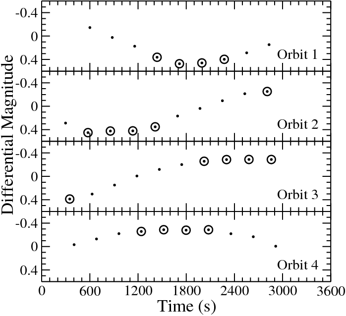
Figure 4: Variability of EF Eri throughout each HST orbit. Each point is a 239s integration, with a differential magnitude computed by dividing the integrated flux by the average flux over all 4 orbits and converting to a magnitude scale. The 9 circled points near minimum light are those used for the minimum flux values (within 23%), and the 9 circled points near maximum light are those within 23% of the maximum flux values.

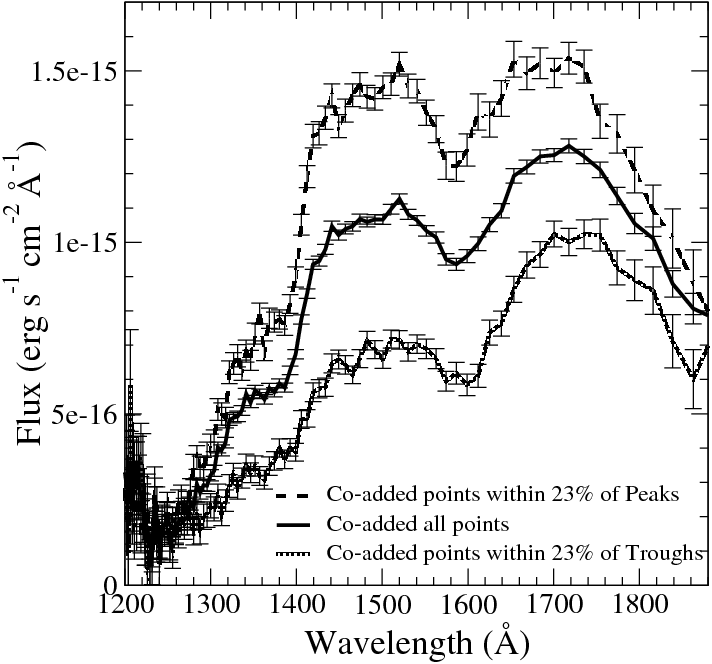
Figure 5: Average spectrum with an extraction width of 17 using all 39 data points (middle solid line), with the 9 points within 23% of the lowest flux points (bottom dotted line) and with the 9 points within 23% of the highest flux points (top dashed line).

The individual HST orbits covered about 0.4-0.5 of the orbital phase of EF Eri on each pass, with all phases covered at least once in the 4 orbit sequence. Figure 4 shows the variability of the flux within each of the four HST orbits. In this plot, each 239s integrated flux point was divided by the average flux, and then converted to a magnitude scale. Due to the large variability throughout the binary orbit of EF Eri, we averaged the spectra in three ways, which are shown in Figure 5. The solid line is the average of all the data, the top dashed line is the average of the 9 integrations within 23% of the peak of the light curves (the highest circled points shown in Figure 4), and the bottom dotted line is the average of the 9 points within 23% of the minimum flux of the light curves (the lowest circled points in Figure 4). The points were selected to avoid the rising and falling portions of the light curve. All three averages show the lowest flux at Ly$\alpha$, a broad minimum near 1600Å, and peaks near 1500 and 1700Å. While these features are preserved in all the averages, the heights of the peaks and the depths of the 1600Å absorption feature change between peak and trough spectra. The 1500Å peak becomes less prominent compared to the 1700Å peak (which causes a corresponding decrease in the depth of the 1600Å absorption feature) during the minimum flux times.

It is possible to interpret these spectra in two ways. If the underlying flux is primarily from a cool white dwarf, the 1600Å absorption can be identified as quasi-molecular hydrogen H₂ which is present in white dwarfs with temperature $\leq$13,500K (Koester et al. 1985). There is also some evidence for quasi-molecular H${}_{2}^{+}$ blueward pf 1400Å, which is present in white dwarfs cooler than 20,000K. Alternatively, if the UV flux comes primarily from cyclotron, the humps at 1500 and 1700Å could be caused by cyclotron harmonics. Support for this origin is the steep decline longward of $\sim$1750Å, which is different from the flatter continuum distribution of a cool white dwarf.

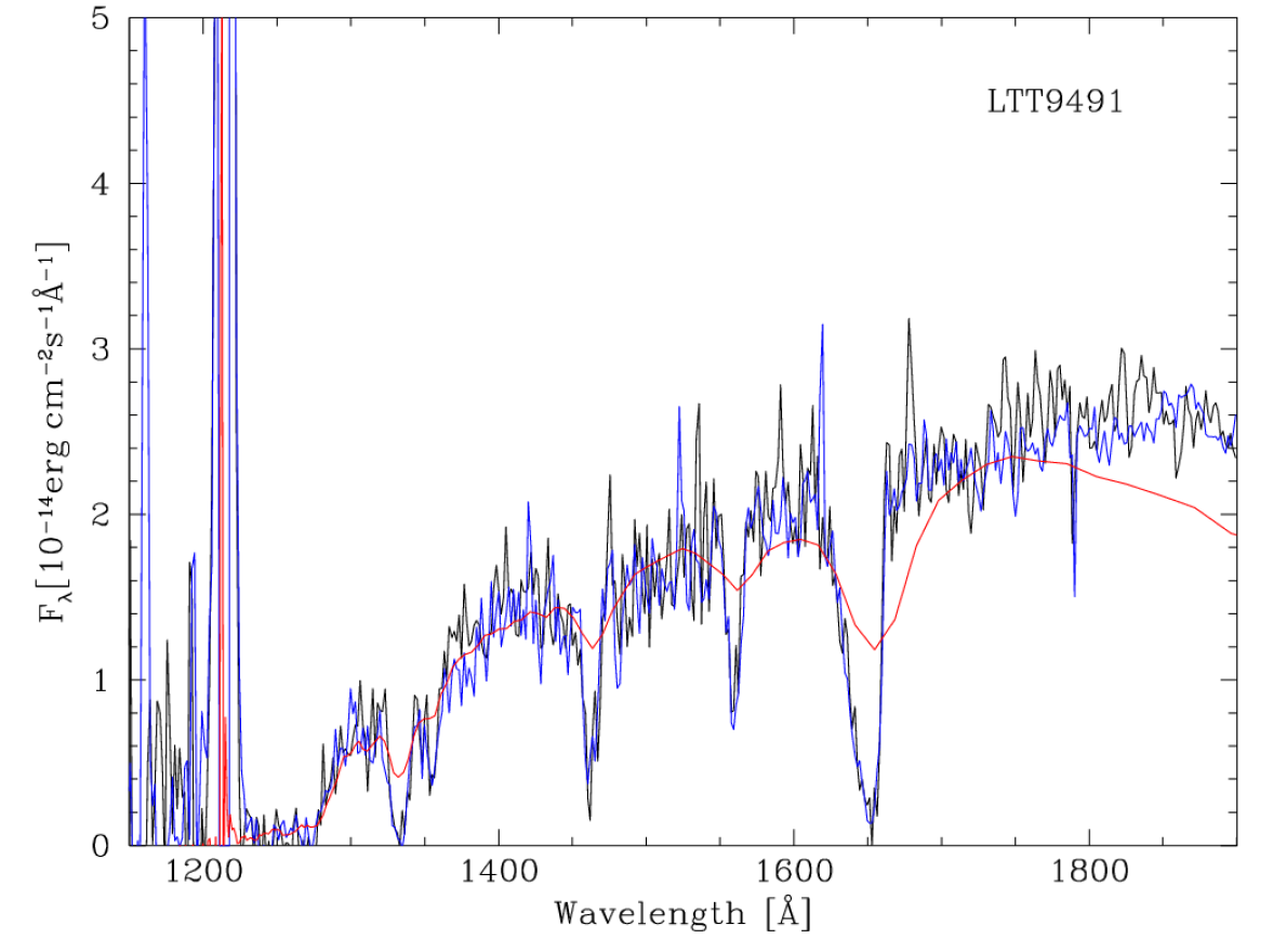
Figure 6: Two IUE spectra of LTT9491 (high resolution lines) compared to the SBC spectrum (low resolution line). Continuum fluxes match well until 1750Å where the SBC flux declines relative to the IUE values by about 30%.

To determine if the drop in flux at longer wavelengths could be a calibration problem, we extracted the SBC spectra of two white dwarf standard stars (WD1657+343 and LTT9491) taken with the PR110L and PR130L prisms from the HST archive. The hot white dwarf WD1657+343 showed a declining spectrum in both prisms from 1250-1850Å while the DZ white dwarf LTT9491 showed a discrepancy longward of 1800Å, with the PR110L spectrum being lower than the PR130L spectrum by 5% at 1850Å. To further check, we extracted two IUE spectra of LTT9491 from the IUE archive (shown in Figure 6 along with the SBC spectrum). This also shows that the SBC calibration is good at short wavelengths but has problems longward of 1750Å. Thus, we regard the calibrated fluxes of EF Eri to be accurate only up to 1750Å.

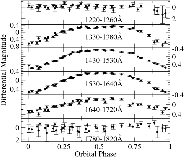
Figure 7: Light curves in 6 UV bands as a function of spectroscopic orbital phase. Each point is the integration of the flux within the bandpass.

For further phase resolution with good S/N, we created light curves as a function of orbital phase by integrating the spectra over the 6 UV bandpasses described in Section 2. These light curves are shown in Figure 7. The bandpasses were chosen to span different features of the spectra. The 1220-1260Å bandpass, which covers the core of Ly$\alpha$, and the 1780-1820Å one, which is the long wavelength downturn in flux, show the least change as a function of the orbit. The bandpasses that include the 1500Å peak (1430-1530Å) and the 1600Å absorption feature (1530-1640Å) have the largest amplitude variablity (over a factor of 2) with peak flux occuring near the same phases as the optical variability (Figures 1 and 2). However, in contrast to the optical, the UV amplitudes are larger and do not show the same asymmetry in shape that is evident in the optical light.

We attempted to model the spectra and the light curves with hot spots on a white dwarf as well as with cyclotron components.

5 Spot Model

Using a similar approach to our modeling efforts for AM Her (Gänsicke et al. 1998, 2006), we used the same code to fit the ACS/SBC light curves of EF Eri. In brief, the surface of the white dwarf is represented by small tiles, with the temperature of each being adjustable. The emission of each tile is described by a white dwarf model spectrum with the corresponding temperature, and the total emission of the white dwarf is computed by integrating the contribution of all tiles on the visible hemisphere. To keep the number of free parameters small, the heated region is represented by a circular spot with an opening angle $\theta_{\rm spot}$, located at a colatitude $\beta_{\rm spot}$ with respect to the rotation axis of the white dwarf, and an $\psi_{\rm spot}$ with respect to the axis connecting the white dwarf and the donor star. The temperature distribution within the spot is assumed to drop linearly in angle from $T_{\mathrm{cent}}$ at the center of the spot to the temperature of the unheated white dwarf, $T_{\mathrm{wd}}$, at the edge of the spot. Koenig et al. (2006) modeled cyclotron heating in the case of AM Her, and found a spot with a flat temperature near the innermost 10^∘, which dropped off approximately linearly out to $\sim$35^∘. For modeling the light curves of EF Eri, a linear drop is the simplest assumption with the smallest number of parameters. Additional parameters are the white dwarf radius $R_{\mathrm{wd}}$, and the distance to the system $d$. We simultaneously fitted the ACS/SBC light curves in wavelength ranges 1330–1380 Å, 1430–1530 Å, 1530–1640 Å, and 1640–1720 Å. The 1220-1260 Å and 1720–1820 Å light curves were omitted from the fit as they were subject to excessive noise and problems in the flux calibration, respectively. Free parameters in the fit were $T_{\mathrm{eff}}$, $R_{\mathrm{wd}}$, $T_{\mathrm{cent}}$, $\theta_{\rm spot}$, $\beta_{\rm spot}$, and $\psi_{\rm spot}$; we kept the distance fixed at $d=120$ pc and the inclination of the binary orbit at $i=50^{\circ}$. The free parameters were adjusted using an evolution strategy (Rechenberg 1994). It carries out a sequence of mutations of the parameters and evaluates them against a fitness function, which we chose to be simply $\chi^{2}$. The step size of the mutation is itself optimized as a function of the convergence of the evolution process. Starting the fit with different initial parameters led to consistent convergence in the six-dimensional parameter space. We list in Table 2 the average values and standard deviations of six solutions found from very different initial start parameters.

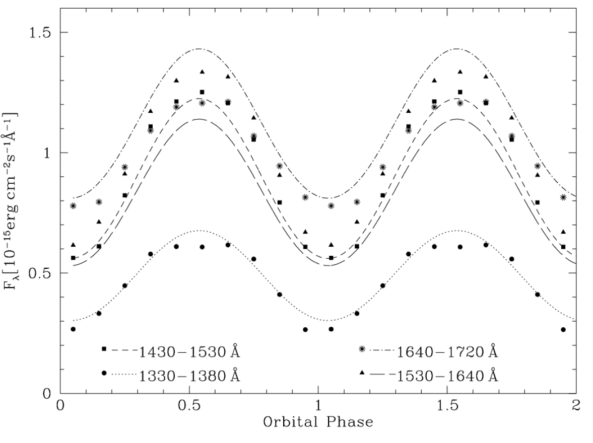
Figure 8: Best fit to the ACS/SBC light curves in four wavelength bands using the white dwarf plus pole cap model. The observed ACS/SBC fluxes are indicated by different symbols, the models corresponding to these bands by different line styles.

Inspecting the best-fit light curves to the ACS/SBC observations (Figure 8) reveals that the 1330–1380 Å data are reasonably well fitted, but that the model significantly over/under predicts the observed fluxes in the three longer wavelength bands. This contrasts with the quality of the fit achieved for the low-state observations of AM Her (Gänsicke et al. 2006). A possible explanation is the presence of some residual ultraviolet flux from low-level accretion, as suggested by the fact that the flux in the core of Ly$\alpha$ (Figure 5) does not drop to zero, as expected for the low temperatures of the white dwarf and its pole cap. However, while the model fails to exactly match the observed fluxes in the four wavelength ranges, it reproduces well the overall spectral shape of the ultraviolet spectra of EF Eri as a function of the orbital phase, i.e. as a function of the geometric projection of the heated pole cap (Figure 8). In particular, the broad depression seen at all phases near 1600 Å corresponds to the quasi-molecular H₂ absorption that occurs in cool, high-gravity atmospheres (Koester et al. 1985, Nelan & Wegner 1985), and the steep rise in flux near 1400 Å observed at orbital maximum is consistent with the quasi-molecular H${}_{2}^{+}$ absorption depressing the flux shortward of 1400Å. There is some uncertainty as to how the magnetic field affects the lines and quasimolecular features in the spectrum of a white dwarf. Gänsicke et al. (2001) have shown that the UV flux distribution of the highest magnetic field polar AR UMa differs greatly from that of non-magnetic white dwarfs in having a flatter UV flux distribution compared to longer optical wavelengths. Overall, the low-state ultraviolet spectrum of EF Eri is rather similar to that of VV Pup ($T_{\mathrm{eff}}=12300$ K, Araujo-Betancor et al. 2005), which also exhibits the 1400 Å and 1600 Å absorption features. The 1600 Å absorption feature disappears in somewhat hotter atmospheres, whereas the 1400 Å feature remains visible up to $\simeq 20\,000$ K (Araujo-Betancor et al. 2005, Gänsicke et al. 2006).

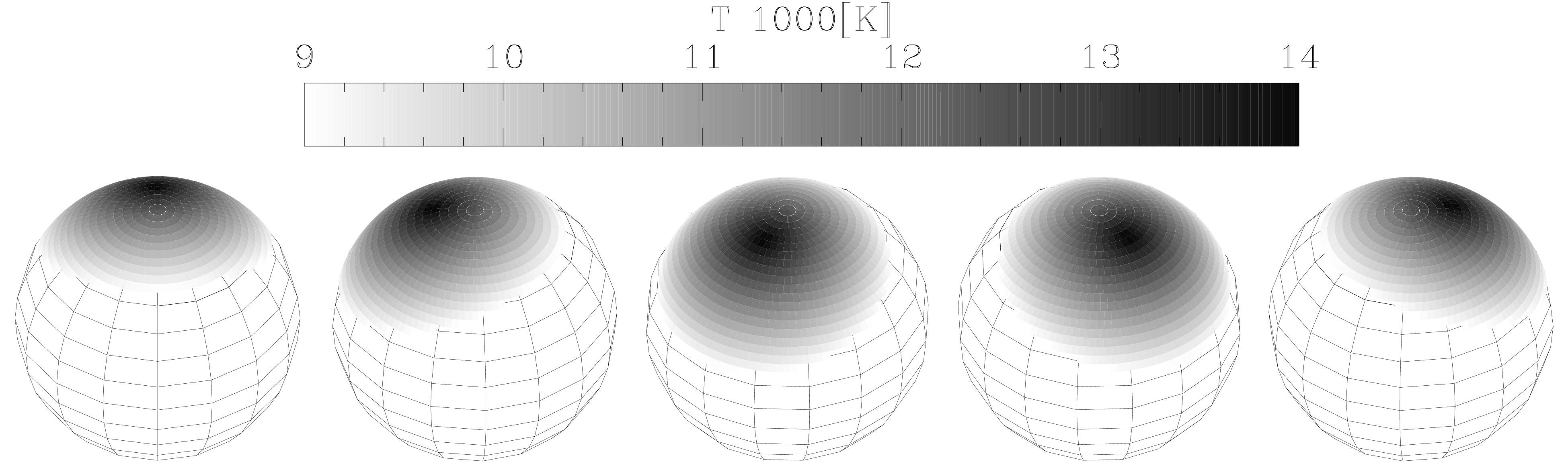
Figure 10: Geometry of the heated pole cap in EF Eri. The unheated white dwarf is represented by grid lines, the pole cap is gray-shaded. Orbital phases are 0.1, 0.3, 0.5, 0.7, and 0.9 (from left to right).

The geometry of the heated pole cap is illustrated in Figure 10. The white dwarf temperature of $\simeq 10000$ K is consistent with the results from the analyses of optical low-state spectroscopy (Beuermann et al. 2000). The white dwarf radius corresponds to a mass of $\simeq 0.8M_{\odot}$, but depends on the assumed distance – a true distance larger (lower) than 120 pc would imply a correspondingly larger, lighter (smaller, heavier) white dwarf. The maximum temperature of the spot, $T_{\mathrm{cent}}\simeq 15000$ K is somewhat lower than the value estimated by Schwope et al. (2007), which was based on the analysis of the orbital-averaged spectral energy distribution of EF Eri as observed with XMM-Newton. Azimuth and co-latitude of the heated pole cap are broadly consistent with the location of the main accretion region in EF Eri as determined by Beuermann et al. (2007) from low-state Zeeman tomography. The fractional area of the heated pole cap in EF Eri is $\sim 22$%, which is larger than that in AM Her (Gänsicke et al. 2006), but comparable to those in V834 Cen, BL Hyi, MR Ser, and V895 Cen (Araujo-Betancor et al. 2005).

6 Cyclotron Model

The cyclotron models were produced using a Constant Lambda (CL) code, which is given a more complete overview in Campbell et al (2008). The underlying algorithm is based on the assumption that the plasma in the accretion column exists in the large Faraday rotation limit $\phi>>1$, where $\phi=\frac{e^{3}\lambda^{2}}{2\pi m^{2}c^{4}}\int_{0}^{s}n_{e}\vec{B}(s)ds$. Radiative transfer therefore decouples into two distinct magnetoionic modes: the ordinary (o) and extraordinary(e), whose optical depths are given by $\tau_{o,e}=\Lambda\phi_{o,e}$, where $\Lambda=l\omega^{2}_{p}/(c\omega_{c})$, where $l$ is the path length through the plasma, $\omega_{p}$ is the plasma frequency, $\omega_{p}=(4\pi Ne^{2}/m)^{1/2}$, and $\omega_{c}$ is the frequency of the cyclotron fundamental, $\omega_{c}=eB/mc$, with $m$ being the relativistic mass of the gyrating particles.

Thus, through the parameter $\Lambda$, it is possible to scale a dimensionless emitting slab to approximate the observed characteristics of a true 3-D cyclotron emission region. However, the model also requires three additional input parameters to calculate the absorption coefficients $\phi_{o,e}$: B, the magnetic field strength, $\Theta$, the angle from the magnetic field line to the line-of-sight of the observer, and kT, the global isothermal temperature of the emitting slab.

Due to the large size of the 4-D parameter space, and the computational effort needed to enumerate and evaluate all points of the search space, an automated optimization routine is required. We used a Genetic Algorithm (GA) to identify the optimal solution (for a good primer on genetic algorithms, see Charbonneau (1995)). GAs are a class of optimization algorithms inspired by biological evolution, these algorithms encode potential solutions on a chromosome-like data structure (called “individuals”) and apply simulated genetic operators to these structures in order to preserve the essential information. GAs begin by establishing a random population of individuals, in our case, always respecting the interval of the 4-D search space. These individuals then evolve through generations by processes of recombination (crossover) and mutation, the natural selection acts at each generation by usually prioritizing individuals with higher scores (most well -adapted), given by the fitness function. While several publicly available GAs frameworks exist, we chose to use Pyevolve for our implementation. Pyevolve is an open-source, modular and object-oriented framework for Evolutionary Computation written in Python language by Christian S. Perone (Perone 2009). Pyevolve is both modular and highly extensible, containing several independent selection schemes which alter how the fitness function is used to populate the next generation.

In our work, the individual was constructed out of the four CL parameters with variants of each parameter randomly selected from within the region defined by [ 65.00 $\leq$B(MG) $\leq$ 125.00, 0.1 $\leq$kT(keV) $\leq$ 25, 0.1 $\leq$log$\Lambda$ $\leq$ 8, 25^∘ $\leq$$\Theta$$\leq$ 85^∘]. A cyclotron model was then run for every individual in the population, and then co-added with a white dwarf (WD) at 120 pc and normalized so that the area under the composite model equals the area under an observed spectrum at a specified phase($\Phi$ = 0.00). To enable direct comparison with the hotspot results, the WD was computed by using the Gänsicke formulation discussed in the previous section, but at a lower temperature of 9500 K. The uncertainty in the temperature is about 1000K around a value of 9750K (Schwope et al. 2007). Since the grid of white dwarf models in our cyclotron fitting had a spacing of 500K, the 9500K point was chosen as closest to the Schwope et al. (2007) value. Our fitness function ranked each individual by looking for the minimum the value of $\chi^{2}_{\nu}$, normalized to the entire population. We employed a Roulette wheel selection scheme, using the Uniform Crossover method with a rate of 90% and a Real Gaussian Mutation method with a rate of 15%. It should be noted that convergence to global minimum requires maintaining genetic diversity over many generations. To this end, a large population of 250 individuals were run against the $\Phi$ = 0.00 data spectrum over 250 generations, finding an optimal solution of $\chi^{2}_{\nu}$ = 1.24 of B = 100 MG, kT = 6.54 keV, log$\Lambda$ = 6.88, and $\Theta$ = 51.26, which took nearly two weeks of computational resources to evaluate.

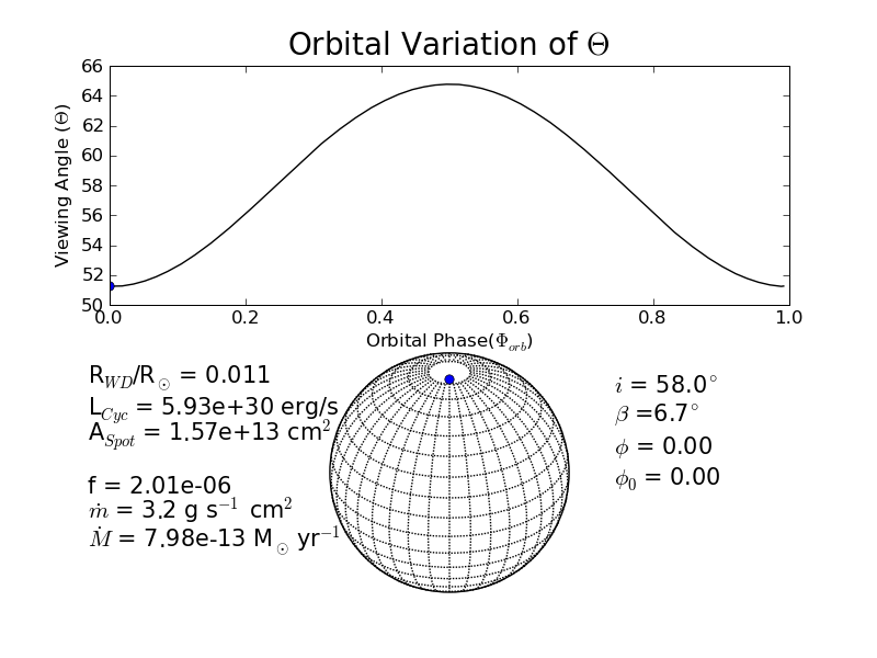
Figure 11: Derived orbital geometry, accretion spot size and accretion rates and the orbital variation of the viewing angle of the magnetic pole. $\phi$ is the current orbital phase and $\phi_{0}$ is maximum light.

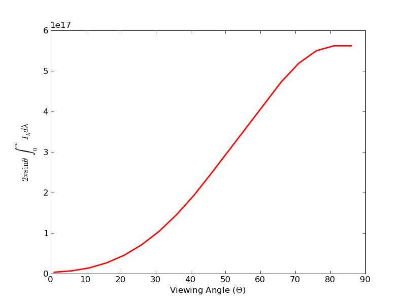
Figure 12: Dependence of the total integrated intensity as a function of the viewing angle $\Theta$. The area under the curve represents the total cyclotron flux.

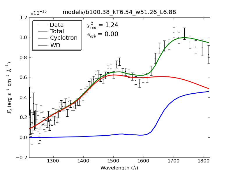
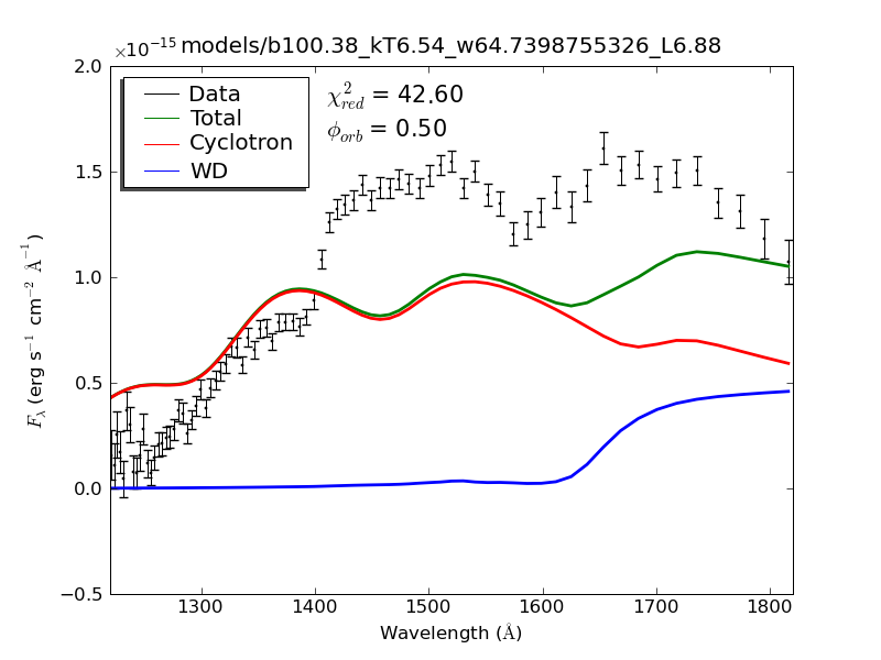
Figure 13: Best fit model spectrum to the phase 0.0 HST spectrum (top) and phase 0.5 HST spectrum (bottom). Data are points with error bars. Lower curves are a 9500K white dwarf, mid curves are the cyclotron component for B=100 MG and top curves are the sum of the two components.

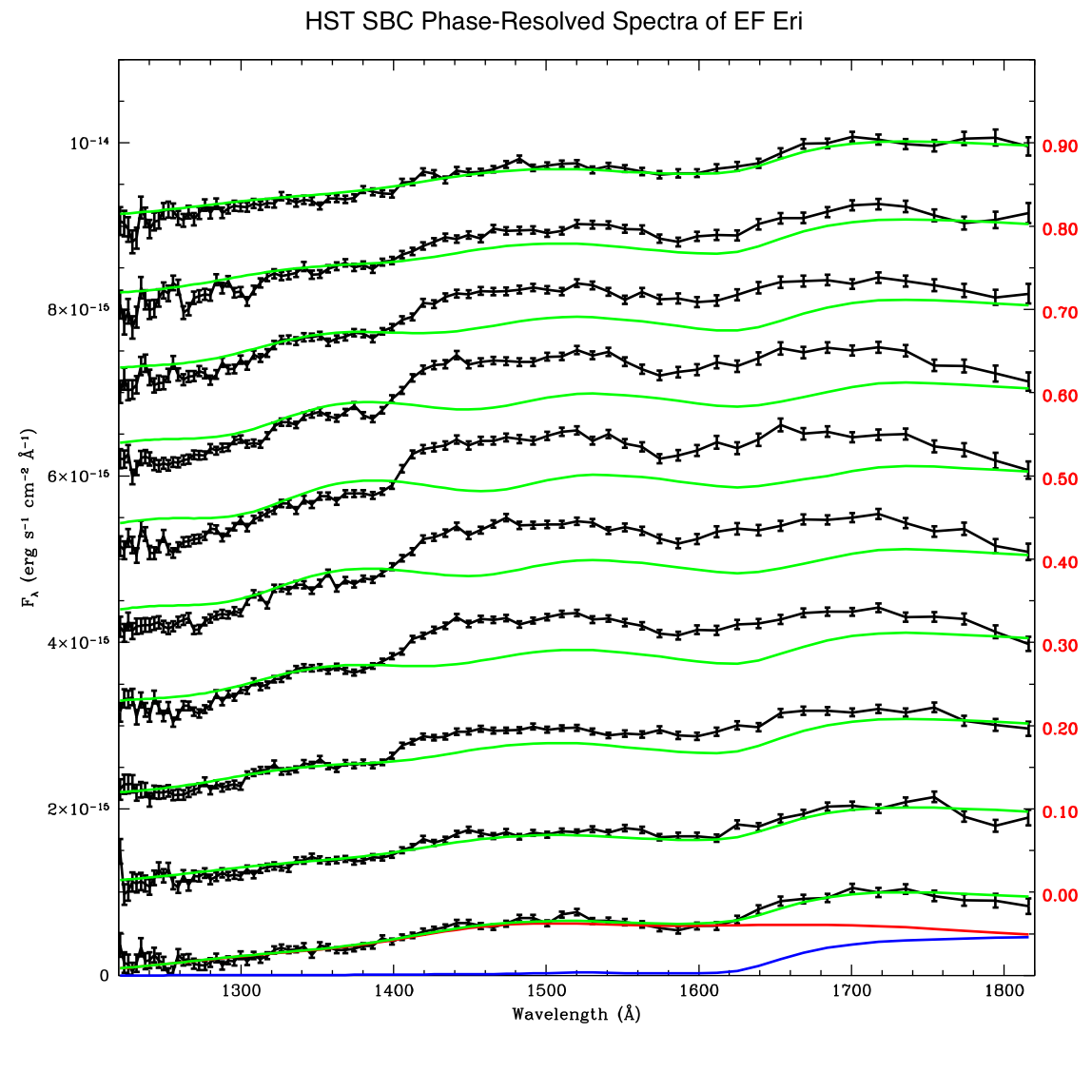
Figure 14: Phase-resolved HST spectra (black with error bars) along with the cyclotron (red), white dwarf (blue) and co-added CYC+WD model (green) for the phase = 0.0 data. Each subsequent phase shows only the data and co-added models. Fluxes at phase 0.0 are real, each subsequent phase has a constant offset of 1$\times$10^-15 added to the flux for clarity of presentation.

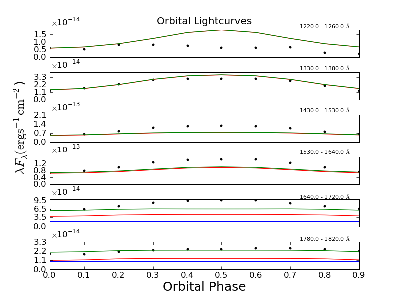
Figure 15: Light curves in 6 bandpasses as a function of orbital phase, with the white dwarf, cyclotron and sum model shown along with the 10 phase points created in each bandpass by integrating the fluxes within each bandpass region listed on the right.

The 39 individual observed spectra of EF Eri were co-added within 0.10 phase bins (with about four spectra within each bin) for comparison to the cyclotron models. Orbital photometry was estimated by integrating these data through six predefined bandpasses. Using an independently determined orbital inclination of $i$ = 58^∘, (Campbell et al. 2008), and the value of $\Theta$ at cyclotron minimum, $\Theta$ = 51.26^∘, is sufficient to constrain the magnetic co-latitude to $\beta$ = 6.7^∘. At every other phase-point, a new cyclotron model was computed keeping B, kT, and log$\Lambda$ constant while allowing $\Theta$ to vary in accordance with the orbital geometry determined above. We then integrated the resulting spectra through each band to produce our lightcurves. Figure 11 shows the optimized parameter set that was determined and the derived quantities while Figure 12 shows cyclotron emission as a function of the viewing angle (the cyclotron beam), with the total flux representing the area under the curve shown. The best-fit model at $\Phi$ = 0.00 is shown in Figure 13 (top). This fit can reproduce the minimum spectra well with B=100 MG, kT=6.54 keV, with $\chi^{2}_{\nu}$ = 1.24. However, the corresponding solution at cyclotron maximum produces a rather poor fit to the observed spectrum at that phase (Figure 13; bottom). The fit to all 10 phases is shown in Figure 14 as a stacked series of spectra, and the integrated light is similarly represented as the light curves for 6 bandpasses in Figure 15. From all possible fits within a large parameter space, we have ruled out a single magnetic component, fixed spot model that can explain the light during the entire orbit. Either variable magnetic field strengths or more than one cyclotron spot would be needed to account for the variability observed. Given that our use of constant $\Lambda$ and kT applied to the whole shock is a simplistic representation of a shock that could have a variety of temperatures, densities and/or magnetic fields, our work is just a first attempt at the problem.

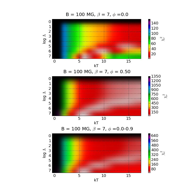
Figure 16: $\chi^{2}$ heat maps of the kT-log$\Delta$ parameter space for B=100 MG and $\beta$=7^∘ at phases 0.0, 0.5 and the average over the entire orbit.

To further ensure that the Pyevolve was converging on the optimal solution, we also ran a large batch of models for B = 100 MG in an evenly spaced grid stepping by ($\Delta$kT, $\Delta$log$\Lambda$) = (1.0,1.0) over the ranges of kT= [0:20] and log$\Lambda$ = [0:8], respectively. The $\chi^{2}_{\nu}$ value for each were then computed at cyclotron minimum, cyclotron maximum, and also averaged over 10 phase-points throughout the orbit. The data were interpolated and mapped to a color scheme to produce heat maps shown in Fig. 16. To orbitally modulate the light-curve, we again varied $\Theta$ to be consistent with an inclination of $i$ = 58^∘, but computed each set of heat maps using various magnetic co-latitudes ($\beta$ = 1, 2, 3 $\dots$ 20^∘) as inputs. $\beta$ = 7^∘ was found to be the optimal solution, where the orbitally averaged heat map had the lowest $\chi^{2}$. A quick inspection of Fig. 16 demonstrates that the Pyevolve is working. Not only has the program converged to the best model at cyclotron minimum (the white spot near kT = 6.54, log$\Lambda$ = 6.88), but an identical solution produces the best model at cyclotron maximum, and indeed averaged through the orbit. Interestingly, while cyclotron minimum has several well defined $\chi^{2}_{\nu}$ minima, the orbital average has no clear best model, presumably because no model fits particularly well.

Finally, we computed the cyclotron flux, F_cyc, luminosity, L_cyc, and specific mass accretion rate, $\dot{m}$. The following recipe was undertaken: (1) Calculate the accretion spot size. Essentially, this is the ratio of the observed cyclotron flux and the raw model intensity both integrated over all wavelengths and subsequently diluted by the surface area of a sphere of radius 120 pc. Normalization to the data was accomplished by scaling to I${}_{\lambda}({\rm Data})$ which is the wavelength integrated model intensity normalized so that the integrated light over the range (1220 $\leq\lambda_{{\rm Data}}\leq$ 1820) equals the integral of the observed fluxes. I${}_{\lambda}({\rm Model})$ is just the integrated raw model intensity. (2) The integrated cyclotron flux was calculated by determining the model intensities at all polar angles, and integrating through both angle and wavelength. (3) L_Cyc is the product of the cyclotron flux and the spot size. (4) The specific mass accretion rate was computed assuming a 0.7 M_⊙ WD, with R_WD determined using the Nauenberg (1972) WD mass-radius relationship. The process is also described numerically below.

$$A_{spot} = \frac{\int_{0}^{\infty}I_{\lambda}({\rm Data}){\rm d}\lambda}{\int_{0}^{\infty}I_{\lambda}(\rm{Model}){\rm d}\lambda}\Big{(}1.20\times 10^{38}d^{2}_{120}\rm{cm}^{2}\Big{)}$$ (1)

$$F_{cyc} = 2\pi\int_{0}^{\frac{\pi}{2}}\int_{0}^{\infty}I_{\lambda}(\Theta)\sin\Theta{\rm d}\theta{\rm d}\lambda$$ (2)

$$L_{Cyc} = F_{cyc}A_{Spot}$$ (3)

$$\dot{m} \approx \frac{L_{cyc}R_{WD}}{GM_{WD}}$$ (4)

From our final results (Figures 13-15), it is obvious that a single cyclotron component can only be fitted to the HST data for a small range in phase (near $\phi$ = 0.00). To fully explain the dataset, it is likely that either a second component is necessary, or the addition of a hotspot is needed. We are reluctant to explore the implications of a second cyclotron component without the inclusion of low-state polarimetry to assess the degree to which the UV emission of EF Eri is polarized.

7 Conclusions

Our low resolution HST spectra have revealed the first UV spectrum of EF Eri during its low accretion state and the corresponding changes in the spectra throughout its orbit. Two interpretations of the lowest orbital UV fluxes at phase 0.0 are possible. If most of the flux is from a white dwarf at a distance of 120 pc, the UV spectrum can be matched with a temperature of $\sim$10,000K and a hot spot with central temperature of 15,000K (similar values found by Beuermann et al. (2000) for the optical region). The broad absorptions at 1400 and 1600Å match those expected for the quasimolecular H features H₂ and H${}_{2}^{+}$ but the flux in the core of Ly$\alpha$ does not go to zero, implying an additional component. On the other hand, the UV spectrum can also be adequately modeled with a 9500K white dwarf at 120 pc that contributes longward of 1600Å in combination with a high (100MG) cyclotron component dominating at the shortest wavelengths.

Both models have difficulty reproducing the observed orbital flux variations, especially for wavelengths longer than 1400Å. A normal white dwarf with a hot spot does not produce enough amplitude near 1500Å  but produces too much flux at 1700Å to account for the phase 0.5 modulation. This type of model has problems producing the amplitudes of the optical flux variations as well. The cyclotron models also require some additional component (either in temperature or in additional field strengths) to account for the phase 0.5 UV fluxes longward of 1400Å. The failure of the simple Constant Lambda model to fit all phases points to the need for more complex multi-temperature, multi-lambda models. While our model excludes a simple UV emitting pole, a more complex accretion region is very possible. The Zeeman tomography work by Beuermann et al (2007) on EF Eri, BL Hyi and CP Tuc shows that the field structures are not simple dipoles and there is a range of field strengths in all three of these polar systems. For EF Eri, the multipole fields range from 4 to 111 MG. This range could accomodate the fields of 13-21 MG that optimally fit the optical and IR spectral regions (Ferrario et al. 1996; Campbell et al. 2008) as well as the UV field strength estimated from ${\it GALEX}$ (Szkody et al. 2008) and our HST data. An additional uncertainty is related to the distance. Ultimately, the choice of model would be best served by UV spectropolarimetry to define the cyclotron component correctly, but a good parallax and UV spectra can pin down the UV luminosity from a high field accreting white dwarf. The theoretical profiles for Ly$\alpha$ and the quasimolecular H features at high fields are not well-known, so observations are currently the best way to determine the influence of the field on the resulting radiation.

Table 1: Observation Summary

UT Date	Observatory	Instrument	Time	Int (s)
2008 Jan 15	NMSU	CCD V filter	02:32-05:34	300
2008 Jan 16	NMSU	CCD V filter	01:27-03:09	300
2008 Jan 16	APO	DIS	01:48-03:30	600
2008 Jan 16	SMARTS	ANDICAM B	02:02:28	100
2008 Jan 17	HST	SBC	10:25-11:01	239
2998 Jan 17	HST	SBC	11:59-12:39	239
2008 Jan 17	HST	SBC	13:35-14:14	239
2008 Jan 17	HST	SBC	15:11-15:50	239
2008 Jan 18	NMSU	CCD V filter	01:31-04:22	300

Table 2: Best-fit Parameters for White Dwarf plus Hot Spot Model

Parameter	Value
$T_{\mathrm{eff}}$	$9850\pm 175$ K
$T_{\mathrm{cent}}$	$15095\,\pm 66$ K
$R_{\mathrm{wd}}$	$(7.95\pm 8)\times 10^{8}$ cm
colatitude ($\beta_{\rm spot}$)	$17.4\pm 1.4^{\circ}$
opening angle ($\theta_{\rm spot}$)	$57.2\pm 2.2^{\circ}$
azimuth ($\psi_{\rm spot}$)	$4.1\pm 0.4^{\circ}$

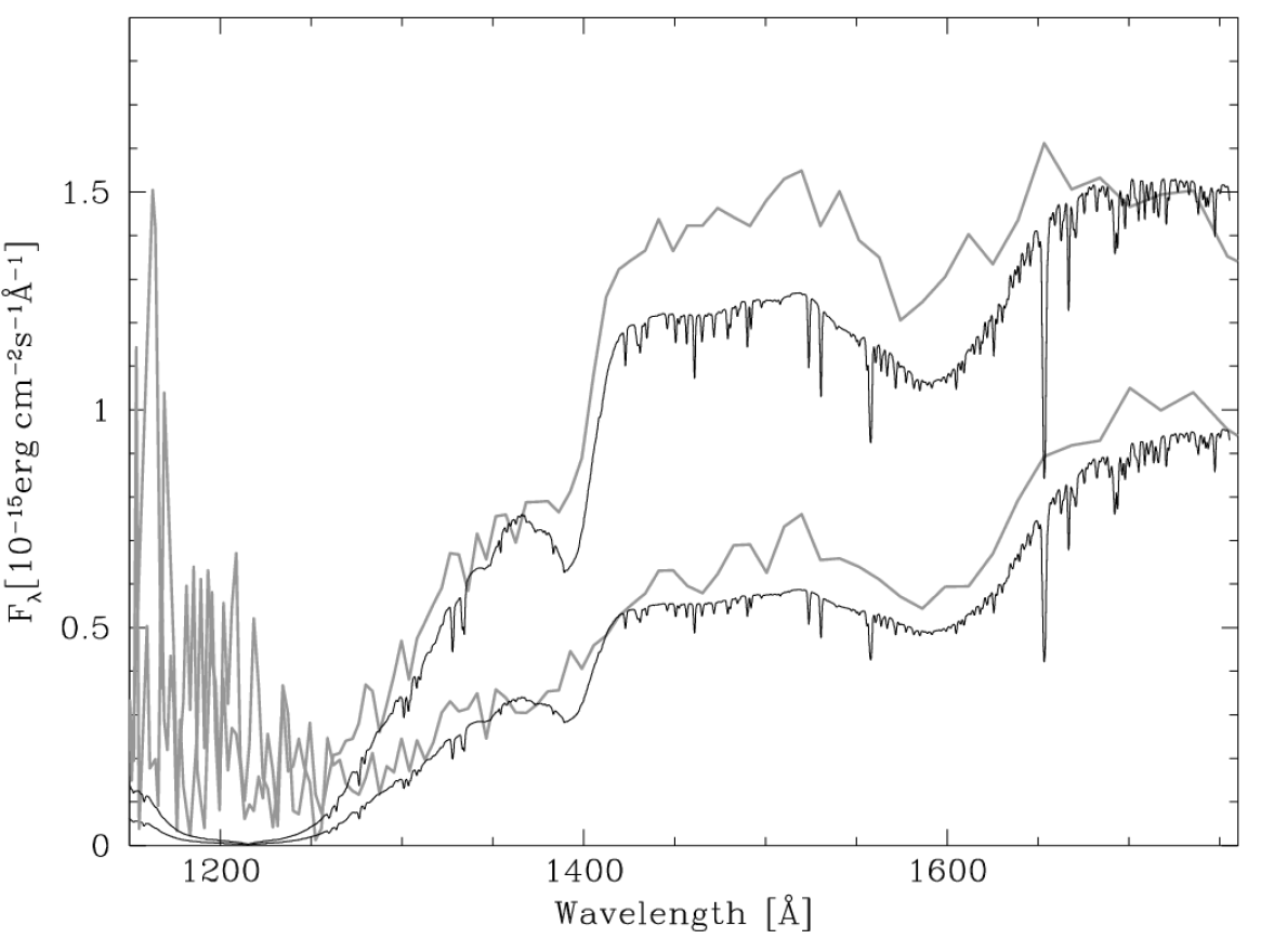
Figure 9: Observed (gray lines) and model spectra at orbital minimum (bottom curves) and orbital maximum (top curves). The model spectra are generated from the best-fit to the ACS/SBC light curves (Figure 7). The broad depressions near 1400 Å and 1600 Å are the quasi-molecular H${}_{2}^{+}$ and H₂ absorptions typical of cool, high-gravity hydrogen atmospheres.

References

- (1)
- (2) Araujo-Betancor, S., et al. 2005, ApJ, 622, 589
- (3) Bailey, J. et al. 1982, MNRAS, 199, 801
- (4) Beuermann, K., Wheatley, P., Ramsay, G., Euchner, F. & Gänsicke, B. T. 2000, A&A, 354, L49
- (5) Beuermann, K., Euchner, F. Reinsch, K., Jordan, S. & Gänsicke, B. T., 2007, A&A, 463, 647
- (6) Campbell, R. K. et al. 2008, ApJ, 672, 531
- (7) Charbonneau, P. 1995, ApJS, 101, 309
- (8) Ferrario, L., Bailey, J. & Wickramasinghe, D. 1996, MNRAS, 282, 218
- (9) Gänsicke, B. T., Beuermann, K. & de Martino, D. 1995, A&A, 303, 127
- (10) Gänsicke, B. T., Beurermann, K., de Martino, D. & Thomas, H.-C. 2000, A&A, 354, 605
- (11) Gänsicke, B. T., Hoard, D. W., Beuermann, K., Sion, E. M. & Szkody, P. 1998, A&A, 338, 933
- (12) Gänsicke, B. T., Schmidt, G. D., Jordan, S. & Szkody, P. 2001, ApJ, 555, 380
- (13) Gänsicke, B. T., Long, K. S., Barstow, M. A. & Hubeny, I. 2006, ApJ, 639, 1039
- (14) Griffiths, R. E. et al. 1979, ApJ, 232, L27
- (15) Harrison, T. E. et al. 2004, AJ, 614, 947
- (16) Heise, J. & Verbunt, F. 1988, A&A, 189, 112
- (17) Hiltner, W. A., Boley, F., Johns, M., Maker, S. Williams, G. IAUC. 3324
- (18) Howell, S. B. et al. 2006a, ApJ, 652, 709
- (19) Howell, S. B. et al. 2006b, ApJ, 646, 665
- (20) King, A. R. & Lasota, J. P. 1979, MNRAS, 188, 653
- (21) König, M., Buermann, K. & Gänsicke, B. T. 2006, A&A, 449, 1129
- (22) Koester, D., Weidemann, V., Zeidler-K. T., E. M. & Vauclair, G. 1985, A&A, 142, L5
- (23) Kuemmel, M., Walsh, J. R., Pirzkal, N., Kuntschner, H. & Pasquali, A. 2009, PASP, 121, 59
- (24) Lamb, D. Q. & Masters, A. R. 1979, ApJ, 234, L117
- (25) Li, J., Wu, K. W. & Wickramasinghe, D. T. 1994, MNRAS, 268, 61
- (26) Li, J., Wicramasinghe, D. T. & Wu, K. W. 1995, MNRAS, 276, 255
- (27) Nauenberg, M. 1972, ApJ, 175, 417
- (28) Nelan, E. P. & Wegner, G. 1985, ApJ, 289, L31
- (29) Perone, C. S. 2009, SIGEVolution, 4, 12
- (30) Rechenberg, I. 1994, Evolutionsstrategie ’94 (Stuttgart:Froomann-Holzboog)
- (31) Rosen, S. R. et al. 2001, MNRAS, 322, 631
- (32) Schwope, A. D. Hambaryan, V., Schwarz, R., Kanback, G., & Gänsicke, B. T. 2002, A&A, 392, 541
- (33) Schwope, A. D., Staude, A., Koester, D. & Vogel, J. 2007, A&A, 469, 1027
- (34) Stockman, H. S., Schmidt, G. D., Liebert, J. & Holberg, J. B. 1994, ApJ, 430, 323
- (35) Szkody, P. et al. 2006, ApJ, 646, L147
- (36) Szkody, P. et al. 2008, ApJ, 683, 967
- (37) Tapia, S. 1979, IAU Circ., 3327
- (38) Thorstensen, J. R. 2003, AJ, 126, 3017
- (39) Walter, F. 2009, 145h N. American Workshop on Cataclysmic Variables and Related Objects
- (40) Wheatley, P. J. & Ramsay, G. 1988, ASPC, 137, 446