Spin Torque Dynamics with Noise in Magnetic Nano-Systems

Abstract

We investigate the role of equilibrium and nonequilibrium noise in the magnetization dynamics on mono-domain ferromagnets. Starting from a microscopic model we present a detailed derivation of the spin shot noise correlator. We investigate the ramifications of the nonequilibrium noise on the spin torque dynamics, both in the steady state precessional regime and the spin switching regime. In the latter case we apply a generalized Fokker-Planck approach to spin switching, which models the switching by an Arrhenius law with an effective elevated temperature. We calculate the renormalization of the effective temperature due to spin shot noise and show that the nonequilibrium noise leads to the creation of cold and hot spot with respect to the noise intensity.

I Introduction

The manipulation of magnetization of a ferromagnet by means of spin-polarized currents is a key issue of the state-of-the-art spintronics concepts (for a review see Ref[Ralph-Stiles, ]). In this respect the most important phenomenon is the so-called spin-transfer-torque (STT) effect, which was predicted by Slonczewski and Berger Slon96 ; Berger : A spin-polarized current may transfer angular momentum to a free ferromagnetic layer resulting in a macroscopic torque on the latter’s magnetization. In very small ferromagnets, in which the magnetization can be assumed spatially uniform, the STT results in the rotation of the magnetization as a whole rather than in the excitation of spin waves. The STT can in particular lead to two dynamical regimes: the reversal of the free layer’s magnetization or a steady state precession of the magnetization. Due to the giant magnetoresistance effect, the dynamics of magnetization is reflected in the change of resistance of the circuit containing magnetic junctions. Current induced resistance variations, identified with STT, were reported in Ref[Tsoi98, ]. In subsequent years both spin torque induced magnetization reversal were observed Myers99 ; Katine00 as well as steady state precession Tsoi00 ; Kiselev03 ; Rippard04 ; Krivorotov . Both dynamical regimes are interesting for applications: as a tempting alternative to Oersted fields in switching the magnetization in ferromagnetic memory elements on the one hand, and as clock devices used to synchronize the CPU with other logic units, on the other. Hence a reliable description of these phenomena is very important.

On a semi-classical level, magnetization dynamics of a mono-domain ferromagnet can be well described by the Landau-Lifshitz-Gilbert Equation (LLG)

$$\frac{\mathrm{d}{\bf m}}{\mathrm{d}t}=-\gamma_{0}{\bf m}\times{\bf H}_{\rm eff}+\alpha_{0}{\bf m}\times\frac{\mathrm{d}{\bf m}}{\mathrm{d}t}+\frac{\gamma_{0}}{M_{s}\mathcal{V}}{\bf m}\times\left({\bf m}\times{\bf I}_{s}\right)\ .$$ (1)

Here ${\bf m}$ is a unit vector in the free layer’s magnetization direction, ${\bf H}_{\rm eff}$ the effective magnetic field, $\mathcal{V}$ the volume of the switching element, $M_{s}$ the absolute value of the free layer’s magnetization, $\gamma_{0}$ the gyromagnetic ratio, $\alpha_{0}$ the Gilbert damping parameter, and ${\bf I}_{s}$ the spin polarized current. However, as the extension of associated devices are very small, effects of noise may play a significant role and should be included into the dynamical description. A first inclusion of noise into the LLG was given in the seminal paper of Brown Brown63 , who considered the effect of thermal fluctuations on the dynamics of a mono-domain particle by a random component ${\bf h}^{R}$ of the effective magnetic field entering the LLG equation (1). As a consequence of the fluctuation-dissipation theorem one finds for the equilibrium correlator of the random field Brown63

$$\langle h_{i}(t)h_{j}(t^{\prime})\rangle\propto\alpha_{0}k_{B}T\delta_{ij}\delta(t-t^{\prime})\ ,$$ (2)

where $h_{i}(t)$ denotes the $i$-th Cartesian component of the random field at time $t$, $k_{B}$ is the Boltzmann constant and $T$ the temperature. Since then, temperature effects on the LLG equation have been considered, both with LiZhang2004 ; Cimpoesu2008 ; ApalkovPRB ; ApalkovJMMM ; Tserkovnyak05 and without the spin torque term Garcia-Palacios ; Scholz . The emphasis of these approaches has been on the influence of noise on switching rates, often by performing explicit numerical calculations Garcia-Palacios ; Scholz ; LiZhang2004 ; Cimpoesu2008 . Since the spin-torque experiments Kiselev03 ; Rippard04 ; Ralph05 ; Rippard06 ; Mistral06 are performed under clear nonequilibrium conditions, it is natural to address, besides temperature, other sources of noise. One possible source of nonequilibrium noise is the spin shot noise. By analogy with the charge shot noise the quantization of the angular momentum transfer leads to spin shot noise, which manifests itself in a random Langevin force entering the equations of motion for the free magnetic layer. It was shown by Foros et al. Tserkovnyak05 in the context of normal metal / ferromagnet / normal metal (NFN) structures that the spin shot noise is the dominant contribution to magnetization noise at low temperatures. In the realistic experiments on spin torque and spin switching the nonequilibrium noise starts to dominate at temperatures below several Kelvins. In Ref[Swie, ] it was shown that inclusion of the nonequilibrium noise into the dynamical description can explain the experimentally obseved nonmonotonic dependence of the microwave power spectrum on the voltage, as well as the saturation of the spectral linewidth at low temperatures.

In this paper we concentrate on the effect of the nonequilibrium noise on spin-switching. Without noise, the spin switching takes place when the spin current (and with it the resulting spin torque) exceeds a critical value. The critical current is determined by the strength of the magnetic anisotropy, external magnetic field and Gilbert damping, and it can be obtained from the solution of the deterministic LLG equation (1). Magnetization noise opens a possibility of activated switching at currents much less than critical. Moreover, in the presence of noise the switching becomes a random process that requires a probabilistic description. The latter is based upon the solution of the Fokker-Planck (FP) equation for the probability distribution of magnetization as derived in Ref[Swie, ]. A crucial step towards this description has been made in Ref[ApalkovPRB, ], where the authors reduced the FP equation for magnetization to the effectively one-dimensional FP equation for the probability distribution of energies and applied it to the description of activated switching processes.

A number of experiments on current induced switching have been carried out previously MyersRaplph2002 ; UrazhdinPRL ; UrazhdinAPL ; Fabian2003 ; WiesendangerScience . From them it was found that the noise reduces the typical switching time, as one might expect. Myers et al. MyersRaplph2002 observed a broad distributions of switching currents strongly depending on temperature, indicating a thermally activated switching process altered by the STT. To fit the measured data they used a Neel-Brown model Brown63 ; Neel with a field- and current-dependent potential barrier height $U(H,I)$. In this model the probability for the magnetization to switch decays exponentially with time over a characteristic relaxation time $\tau$ that obeys the Arrhenius law $\tau\sim e^{U/k_{B}T}$. An implicit assumption in the Neel-Brown theory is that magnetization dynamics is governed by a torque from an effective magnetic field ${\bf H}_{\rm eff}$, which is derivable from the free energy $E({\bf M})$ of the system via ${\bf H}_{\rm eff}=-\frac{1}{\mu_{0}}{\bf\nabla}_{M}E({\bf M})$. The spin torque however is non-conservative and the concept of a corresponding potential barrier is ill-defined, which makes the situation significantly more complicated. For thermally activated switching in presence of STT Urazhdin et al. UrazhdinPRL ; UrazhdinAPL found that the activation energy strongly depends on the magnitude as well as the direction of the current. To capture the observed features they introduced an effective temperature distinct from the real temperature in the Neel-Brown formula. Its current directional dependence indicated that the heating is not the ordinary Joule heating. Based on a stationary solution of the Fokker-Planck equation Apalkov and Visscher ApalkovPRB ; ApalkovJMMM , and Li and Zhang LiZhang2004 , linked this effective temperature to the spin torque. In their model the alteration of switching rates is due to the change of the elevated effective temperature in the Arrhenius factor, which in general yields a non-Boltzmann probability distribution. We extend the approach of Ref[ApalkovPRB, ] considering the influence of the noise on the switching in the whole range of currents, from the noise induced activated switching at small currents up to the almost deterministic switching by large critical currents. We also take into account specific angular dependence of the nonequilibrium noise and analyze the applicability of the effective temperature description to the nonequilibtium noise in detail.

With the present paper we hope to give a contribution towards a better understanding of noise in magnetic systems. In section II we start our discussion with a detailed derivation of the spin shot noise correlator by means of the Keldysh technique. It is our goal to depict the underlying mechanisms that lead to the occurrence of spin shot noise in magnetic nanodevices and to provide a general mathematical framework for their description. We then turn our attention to the ramifications of the noise on the magnetization dynamics. We address the question of switching rates estimation in sections III and IV by applying a generalized Fokker-Planck approach. Within this approach the alteration of switching rates due to spin torque is determined by an effective temperature $T_{\rm eff}$. The latter differs from the real temperature $T$, as it incorporates the effects of the damping, the spin torque, and noise. We calculate the renormalization of the effective temperature due to the nonequilibrium noise. A conclusion of our findings is given in section V.

II Spin Shot Noise Correlator

In this section, starting from a microscopic model of a magnetic tunnel junction (MTJ) we will derive a stochastic version of the LLG equation. Fluctuations will naturally come about due to the nonequilibrium situation, and will comprise the random part of the stochastic LLG. In particular, performing a perturbative expansion of the Keldysh action in terms of the spin flip processes and the tunneling amplitude we will be able to derive the spin shot noise correlator.

The model MTJ consists of two itinerant ferromagnets separated by a tunneling barrier. Let us introduce the corresponding model Hamiltonian allowing for an external magnetic field ${\bf H}$, tunneling of itinerant electrons through the barrier and exchange coupling between the itinerant electrons and the free layer’s magnetization. It reads

$$H_{0}= \sum_{k,\sigma}\epsilon_{k\sigma}c^{\dagger}_{k\sigma}c_{k\sigma}+\sum_{l\sigma}\epsilon_{l}d^{\dagger}_{l\sigma}d_{l\sigma}-\gamma{\bf S}\cdot{\bf H}-2J\,{\bf S}\cdot{\bf s}$$

$$+\left[\sum_{kl\sigma}W_{kl}c^{\dagger}_{k\sigma}d_{l\sigma}+h.c.\right]\,.$$ (3)

The notation is as follows: The creation (annihilation) operators $c^{\dagger}_{k\sigma}$ ($c_{k\sigma}$) and $d^{\dagger}_{l\sigma}$ ($d_{l\sigma}$) describe the itinerant electrons of the fixed and the free magnetic layer respectively. $\sigma=+$ corresponds to the respective majority and $\sigma=-$ to the minority spin band, and the indices $k$ and $l$ label momentum. The operator ${\bf S}$ describes the total spin of the free layer. It is connected to the free layer’s magnetization via ${\bf S}={\bf M}{\cal V}/\gamma$. ${\bf s}=\frac{1}{2}\sum_{l\sigma\sigma^{\prime}}d^{\dagger}_{l\sigma}\vec{\sigma}_{\sigma\sigma^{\prime}}d_{l\sigma^{\prime}}$ is the quantum operator associated with the spin of itinerant electrons, where $\vec{\sigma}$ denotes the vector of Pauli matrices. $J$ is the exchange coupling constant and $W_{kl}$ are tunneling matrix elements.

For the subsequent discussion we assume that the time between two tunneling processes is much larger than the relaxation time in the free ferromagnet, which is equivalent to assuming a complete spin relaxation in the free magnetic layer. This allows us to introduce an instantaneous reference frame with the spin quantization axis directed along the free layer’s magnetization direction. To render the free layer’s magnetization a dynamical variable, we make use of the Holstein-Primakoff parametrization Holstein-Primakoff

$$S_{z}=S-b^{\dagger}b;\ \ S_{-}=b^{\dagger}\sqrt{2S-b^{\dagger}b};\ \ S_{+}=\sqrt{2S-b^{\dagger}b}\,b,$$ (4)

where $b^{\dagger},b$ are usual bosonic operators and $S_{\pm}=S_{x}\pm iS_{y}$. At low temperatures we can assume that the expectation value of $b^{\dagger}b$ is much smaller than $2S$ allowing to treat the square root to zeroth order in $b^{\dagger}b$. Taking all of the above mentioned into account, Hamiltonian (II) can be written in the instantaneous reference frame as

$$H_{0}=\sum_{k,\sigma}\epsilon_{k\sigma}c^{\dagger}_{k\sigma}c_{k\sigma}+\sum_{l\sigma}(\epsilon_{l}-JS\sigma)d^{\dagger}_{l\sigma}d_{l\sigma}-\gamma SH_{z}$$

$$+\gamma b^{\dagger}bH_{z}+Jb^{\dagger}b\sum_{l\sigma}\sigma d^{\dagger}_{l\sigma}d_{l\sigma}+\left[\sum_{kl,\sigma\sigma^{\prime}}W_{kl}^{\sigma\sigma^{\prime}}c^{\dagger}_{k\sigma}d_{l\sigma^{\prime}}\right.$$

$$\left.-\,b\sqrt{2S}\left(J\sum_{l}d^{\dagger}_{l\downarrow}d_{l\uparrow}+\frac{\gamma}{2}H_{-}\right)+h.c.\right]\,,$$ (5)

where we used the notation $H_{\pm}=H_{x}\pm iH_{y}$. $W_{kl}^{\sigma\sigma^{\prime}}$ are spin dependent tunneling matrix elements given by

$$W_{kl}^{\sigma\sigma^{\prime}}=\langle\sigma|\sigma^{\prime}\rangle W_{kl},$$ (6)

$$\langle\sigma|\sigma\rangle=\cos\tfrac{\theta}{2}e^{-\frac{i}{2}\sigma\phi},\quad\langle\sigma|\sigma^{\prime}\rangle=\sigma^{\prime}\sin\tfrac{\theta}{2}e^{\frac{i}{2}\sigma\phi}\ .$$ (7)

Hamiltonian (II) can be now readily translated into a Keldysh action using the general scheme of the Keldysh technique Kamenev05 . To this end we switch to symmetric (”$cl$”) and antisymmetric (”$q$”) linear combinations of the field operators. In accordance with parametrization (4) the former are connected to the $m_{\pm}$ components of the free layer’s magnetization in the instantaneous reference frame via

$$b_{cl}(t)=\sqrt{\frac{M_{s}\mathcal{V}}{2\gamma}}\,m_{+}(t)\ ,\qquad\bar{b}_{cl}(t)=\sqrt{\frac{M_{s}\mathcal{V}}{2\gamma}}\,m_{-}(t)\ .$$ (8)

For the retarded and advanced components of the fermionic Green functions for the itinerant electrons of the free and fixed layer we obtain in the energy domain

$$G^{R/A}_{l\sigma}=\frac{1}{\epsilon-\epsilon_{l\sigma}\pm i0}\ ,\qquad G^{R/A}_{k\sigma}=\frac{1}{\epsilon-\epsilon_{k\sigma}\pm i0}\ ,$$ (9)

where $\epsilon_{l\sigma}=\epsilon_{l}-\sigma JS$ are the energies of the itinerant electrons with momentum $l$ and spin $\sigma$ in the free ferromagnet, and $\epsilon_{k\sigma}$ the corresponding energies for the fixed layer. The Keldysh components are

$$G^{K}_{l\sigma}=(1-2n^{d}_{F}(\varepsilon))\delta\left(\epsilon-\epsilon_{l\sigma}\right),$$ (10)

$$G^{K}_{k\sigma}=(1-2n^{c}_{F}(\varepsilon))\delta\left(\epsilon-\epsilon_{k\sigma}\right),$$ (11)

where chemical potentials $\mu_{d/c}$ for the free and fixed layer are included in the fermionic distribution functions $n_{F}^{c/d}$. For future use we also define the matrices in Keldysh space

$$\gamma^{cl}=\begin{pmatrix}1&0\\ 0&1\end{pmatrix}\ ,\qquad\gamma^{q}=\begin{pmatrix}0&1\\ 1&0\end{pmatrix}\ .$$ (12)

The Keldysh action can be now solved perturbatively in terms of the tunneling amplitude and the spin flip processes. In second order in both quantities this leads to the diagrams of Fig. 1. The corresponding equations of motion are obtained when varying the action $\mathcal{A}$ with respect to the quantum component

$$\frac{\delta\mathcal{A}}{\delta b_{q}}=0\ ,\qquad\frac{\delta\mathcal{A}}{\delta\bar{b}_{q}}=0\ .$$ (13)

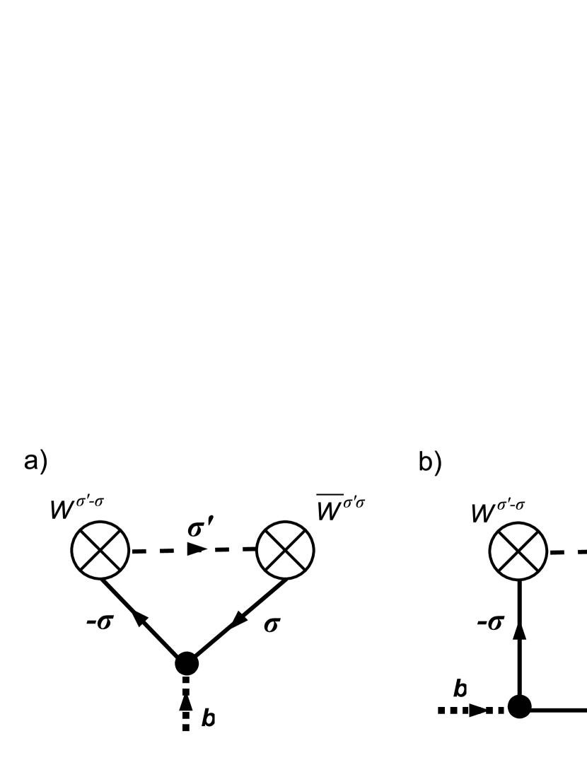
Figure 1: (Color Online) Diagrams for spin flip processes: a) First order. b) Second order. Solid (dashed) lines denote electronic propagators in the free (fixed) layer. Bold dashed lines are propagators of HP bosons. Tunneling vertices are denoted by circles with crosses.

Finally we note that, in the instantaneous reference frame, we have for $m_{\pm}=m_{x}\pm im_{y}$

$$\langle m_{\pm}\rangle=0\ ,\qquad\langle\partial_{t}m_{\pm}\rangle\neq 0\ ,$$ (14)

where, on the other hand

$$\langle m_{z}\rangle=1\ ,\qquad\langle\partial_{t}m_{z}\rangle=0\ .$$ (15)

We may now translate diagrams 1 (a) and (b) into the analytical expressions. However, let us start with the contribution of zeroth order (in spin flips and in tunneling). It reads

$$\mathcal{A}_{0}=\int\mathrm{d}t\bar{b}_{q}(t)\left(i\partial_{t}b_{cl}(t)+\gamma\sqrt{S/2}H_{+}\right)+\rm{c.~{}c.}$$ (16)

The resulting equations of motion are

$$i\partial_{t}b_{cl}+\gamma\sqrt{S/2}H_{+}=0$$ (17)

and a corresponding complex conjugate equation for $\bar{b}_{cl}$. Equation (17) describes the precession of the magnetization around the magnetic field ${\bf H}$ and forms the first term of the LLG equation (1).

Let us come to the diagram of Fig. 1(a). To extract its contribution to the action we have to calculate

$$-J\sqrt{S}\sum_{kl\sigma\sigma^{\prime}}W_{kl}^{\sigma^{\prime}-\sigma}\bar{W}_{kl}^{\sigma^{\prime}\sigma}b_{\sigma}\mathrm{Tr}\left\{G^{d}_{l\sigma}\gamma^{q}G^{d}_{l-\sigma}G^{c}_{k\sigma^{\prime}}\right\}\ ,$$ (18)

where for brevity the symbolic notation $b_{\sigma}$ with $b_{\uparrow}=b_{q}$ and $b_{\downarrow}=\bar{b}_{q}$ was introduced. The resulting action reads

$$\mathcal{A}_{1}=\frac{i}{2\sqrt{S}}I_{s}\int\mathrm{d}t\left\{\bar{b}_{q}(t)\sin\theta e^{-i\phi}-b_{q}(t)\sin\theta e^{i\phi}\right\}\ .$$ (19)

Variation of (19) with respect to $b_{q}$ and $\bar{b}_{q}$ gives the following contribution to the equations of motion

$$\frac{\delta\mathcal{A}_{1}}{\delta b_{q}(t)} =-i\frac{I_{s}}{\sqrt{2S}}\sin\theta e^{i\phi}\ ,\qquad\frac{\delta\mathcal{A}_{1}}{\delta\bar{b}_{q}(t)}=i\frac{I_{s}}{\sqrt{2S}}\sin\theta e^{-i\phi}\ .$$ (20)

Again, using the HP parametrization (4) and the relation between ${\bf S}$ and ${\bf m}$, equation (20) can be readily translated into the corresponding equation of motion for the magnetization. The result is the spin torque term of equation (1)

$$\partial_{t}{\bf m}=\frac{\gamma}{M_{s}\mathcal{V}}{\bf m}\times\left({\bf I}_{s}\times{\bf m}\right)\ .$$ (21)

As far as the remaining diagram (Fig. 1(b)) is concerned we have to distinguish two contributions: One with two quantum components and one with a quantum and a classical component respectively. In the first case we obtain

$$J^{2}Sb_{q}\bar{b}_{q}\sum_{kl\sigma\sigma^{\prime}}|W^{\sigma^{\prime}-\sigma}_{kl}|^{2}\mathrm{Tr}\left\{G^{d}_{l-\sigma}(\varepsilon)\gamma^{q}G^{d}_{l\sigma}(\varepsilon-\omega)\times\right.$$

$$\left.\gamma^{q}G^{d}_{l-\sigma}(\varepsilon)G^{c}_{k\sigma^{\prime}}(\varepsilon)\right\}\ .$$ (22)

In the second case we have

$$J^{2}Sb_{cl}\bar{b}_{q}\sum_{kl\sigma\sigma^{\prime}}|W^{\sigma^{\prime}-\sigma}_{kl}|^{2}\mathrm{Tr}\left\{G^{d}_{l-\sigma}(\varepsilon)\gamma^{q}G^{d}_{l\sigma}(\varepsilon-\omega)\times\right.$$

$$\left.\gamma^{cl}G^{d}_{l-\sigma}(\varepsilon)G^{c}_{k\sigma^{\prime}}(\varepsilon)\right\}\ ,$$ (23)

and the corresponding contribution with $q\leftrightarrow cl$. The resulting action is

$$\mathcal{A}_{2}=\int\mathrm{d}t\left[\bar{\alpha}(\theta)\left(\bar{b}_{q}\partial_{t}b_{cl}-\bar{b}_{cl}\partial_{t}b_{q}\right)+\frac{2i}{S}\mathcal{D}(\theta)\bar{b}_{q}b_{q}\right]\ ,$$ (24)

where

$$\bar{\alpha}(\theta) =\frac{\hbar\gamma}{eM\mathcal{V}}\left(\frac{\mathrm{d}I_{sf}(\theta)}{\mathrm{d}V}\right)\ ,$$ (25)

$$\mathcal{D}(\theta) =\frac{M_{s}\mathcal{V}}{\gamma}\alpha_{0}k_{B}T+\frac{\hbar}{2}\,{\rm I}_{sf}(\theta)\coth\left(\frac{eV}{2k_{B}T}\right)\,.$$ (26)

The spin flip current ${I}_{sf}$ can be calculated from the electric conductances $G_{P(AP)}$ in the parallel (antiparallel) configuration as follows

$$\frac{\mathrm{d}I_{sf}(\theta)}{\mathrm{d}V}=\frac{\hbar}{4e}\left[G_{P}\sin^{2}\left(\frac{\theta}{2}\right)+G_{AP}\cos^{2}\left(\frac{\theta}{2}\right)\right]\ .$$ (27)

Action (24) consists of two parts. The first term is a damping term. In the LLG equation it will result in a renormalization of the Gilbert damping parameter. The renormalization is due to the coupling to the reservoirs. The enhancement of the damping, Eq. (25), is closely related to the spin-pumping enhanced damping as discussed in Ref[Tserkovnyak02, ; Halperin-Tserkovnyak, ] in the framework of the Landauer-Büttiker formalism. As far as the second term of Eq.(24) is concerned we introduce a Hubbard-Stratonovich auxiliary field which decouples the action. Let us denote this (complex) field by ${I}^{R}_{+}=I^{R}_{s,x}+iI^{R}_{s,y}$. We can write

$$\int\mathrm{d}I^{R}_{+}\mathrm{d}\bar{I}^{R}_{+}\,e^{-\frac{1}{4\mathcal{D}}I^{R}_{+}\bar{I}^{R}_{+}}\,e^{i\mathcal{A}_{21}}\\ =\int\mathrm{d}I^{R}_{+}\mathrm{d}\bar{I}^{R}_{+}\,e^{-\frac{1}{4\mathcal{D}}I^{R}_{+}\bar{I}^{R}_{+}}\,\exp\left\{-i\tfrac{1}{\sqrt{2S}}(I^{R}_{+}\bar{b}_{q}+\bar{I}^{R}_{+}b_{q})\right\}\ ,$$ (28)

where we abbreviated the second term of (24) by $\mathcal{A}_{22}$. As one can see the result is a noise-averaged term which is linear in the quantum component. The linear action constitutes a resolution of functional $\delta$-functions of the Langevin equations on $b_{cl}(t)$ and its complex conjugate. The stochastic properties are encoded in the auxiliary field ${I}^{R}_{+}$, precisely in the correlator (26). For $b_{cl}$ the Langevin equations read $i\partial_{t}b_{cl}=\tfrac{1}{\sqrt{2S}}I^{R}_{+}$. This corresponds to $i\partial_{t}m_{+}=\tfrac{\gamma}{M\mathcal{V}}I^{R}_{+}$ leading to the random term of the stochastic LLG equation. Adopting the notation ${\bf I}^{R}_{s}\equiv\delta{\bf I}_{s}$, in conclusion we have found

$$\partial_{t}{\bf m}\,=\frac{\gamma}{M_{s}\mathcal{V}}{\bf m}\times\left(\delta{\bf I}_{s}\times{\bf m}\right)\ ,$$ (29)

where the stochastic field is characterized by

$$\langle\delta{I}_{s,i}(t)\delta{I}_{s,j}(t)\rangle=2\mathcal{D}(\theta)\delta_{ij}\delta(t-t^{\prime})\$$ (30)

with the correlator $\mathcal{D}(\theta)$ given by Eq. (26).

To complete our discussion we add some comments concerning the correlator (26). To start with, we note that $\mathcal{D}$ contains two parts, an equilibrium part (which is phenomenological, and in compliance with the FDT proportional to $\alpha_{0}$ taking into account intrinsic damping processes) and a nonequilibrium part. The nonequilibrium part exhibits a dependence on the mutual orientation of the fixed and free layer’s magnetizations. This angle dependence enters the correlator through the spin flip current $I_{sf}$. The physical meaning behind this quantity is the following: $I_{sf}$ counts the total number of spin flip events, irrespective of their direction. Hence, even if there is no contribution to the spin current $I_{s}$, the spin flip current $I_{sf}$ may acquire a nonzero value. The discreteness of angular momentum transfer in each spin flip event leads to the occurrence of the nonequilibrium noise. In this sense the nonequilibrium part of (26) can be identified with the spin shot noise.

In conclusion we have derived the following stochastic LLG equation

$$\frac{\mathrm{d}{\bf m}}{\mathrm{d}t}=-\gamma_{0}{\bf m}\times{\bf H}_{\rm eff}+\alpha_{0}{\bf m}\times\frac{\mathrm{d}{\bf m}}{\mathrm{d}t}+\frac{\gamma_{0}}{M_{s}\mathcal{V}}{\bf m}\times\left[{\bf m}\times\left({\bf I}_{s}+{\bf I}^{R}_{s}\right)\right]\ ,$$ (31)

where the random field correlator is given by Eq. (30) along with (26) and (27) .

III Fokker-Planck Approach to Spin Torque Switching

Spin torque switching is observable in two different regimes. On the one hand, the spin torque can switch the magnetization of a free ferromagnet when the current exceeds a critical value $I_{c}$. On the other hand, switching is also observed for currents below $I_{c}$. In the second case the actual switching procedure is mainly noise induced. A suitable description of switching times in this regime can be obtained from the Fokker-Planck approach which was recently introduced by Apalkov and Visscher in the context of thermal fluctuations ApalkovPRB ; ApalkovJMMM . Within this approach switching rates are specified by an Arrhenius like law with an effective temperature $T_{\rm eff}$. The latter differs from the real temperature $T$, as it is influenced by the damping and the spin torque. In the sequel we present a generalization of the method to nonequilibrium noise, and show that the spin shot noise alters the effective temperature.

Let us start our consideration with the Fokker-Planck equation as introduced by Brown Brown63 . We denote the probability density for the magnetization of a mono-domain particle by $\rho({\bf m},t)$. The corresponding Fokker-Planck equation can be written in the form of a continuity equation

$$\frac{\partial\rho({\bf m,t})}{\partial t}=-{\bf\nabla}\cdot{\bf j}({\bf m},t)$$ (32)

with probability current Brown63

$${\bf j}({\bf m},t)=\rho({\bf m},t){\bf\dot{m}}_{det}({\bf m})-D{\bf\nabla}\rho({\bf m},t)\ .$$ (33)

Here ${\bf\dot{m}}_{det}$ denotes the deterministic part of the stochastic LLG (1) and $D$ is the random field correlator. We recall that the dynamics governed by (1) conserves the absolute value of ${\bf m}$. As a consequence the movement of the tip of ${\bf m}$ is restricted to the surface of a sphere, which we will call the $m$-sphere. The gradient and the divergence in (32) and (33) are 2-dimensional objects, both living on the $m$-sphere.

We now observe that in presence of anisotropy the phase space will be in general separated. The potential landscape will exhibit different minima referring to stable and meta-stable states of the magnetization. Precession of the magnetization takes place around one (or more) of these equilibrium positions. We refer to orbits of constant energy as Stoner-Wohlfarth (SW) orbits. Now, considering the dynamics of the magnetization vector one can distinguish two different time scales. The time scale for the angular movement, on the one hand, is characterized by the precession frequency. On the other hand there is also a time scale for a possible change in energy. In the following we will require that the time scale for the change in energy is much longer than the time scale for constant energy precession. In other words: we assume that the magnetization vector stays rather long on a SW orbit before changing to higher/lower energies. In this low damping and small current limit we can introduce an energy-dependent probability density by identifying $\rho^{\prime}_{i}(E({\bf m}),t)\equiv\rho({\bf m},t)$, where the index $i$ takes into account that the energy dependence may be different in different regions of the $m$-sphere. The above mentioned time scale separation allows us to average out the movement along the SW orbit and to be concerned with only the long time dynamics.

The idea of the FP approach is to translate equation (32) into a corresponding equation for $\rho^{\prime}_{i}(E)$. For thermal noise this has been done in Ref[ApalkovPRB, ]. We now give a generalization of the method to the angle-dependent spin shot noise of section II. To this end we write the correlator (26) in the form

$$D(\theta)=D_{th}+D_{0}\left[1-P\cos\theta\right]\ ,$$ (34)

where $D_{th}=\frac{\gamma\alpha k_{B}T}{M_{s}\mathcal{V}}$ is the thermal part and $D_{0}[1-P\cos\theta]$ the nonequilibrium part of the correlator.

We abbreviated the angle-independent part of the spin shot noise by $D_{0}$. We also used

$$P=\frac{G_{P}-G_{AP}}{G_{P}+G_{AP}}\ .$$ (35)

In general we can write the Fokker-Planck equation for the distribution $\rho^{\prime}_{i}(E({\bf m}),t)$ in the form ApalkovPRB

$$\frac{\gamma P_{i}(E)}{M_{s}\mu_{0}}\frac{\partial\rho_{i}^{\prime}(E,t)}{\partial t}=-\frac{\partial}{\partial E}j^{E}_{i}(E,t)\ ,$$ (36)

where $P_{i}(E)$ is the period of the orbit with energy $E$. $j^{E}_{i}$ is the probability current in energy. It is given by

$$j^{E}_{i}(E,t)=\oint[{\bf j}({\bf m},t)\times d{\bf m}]\cdot{\bf m}=-\gamma\alpha\rho^{\prime}_{i}(E,t)I^{E}_{i}(E)$$

$$+\gamma J\rho^{\prime}_{i}(E,t){\bf m}_{p}\cdot{\bf I}^{M}_{i}-\frac{\partial\rho^{\prime}(E)}{\partial E}M_{s}D_{th}I^{E}_{\theta,i}\ .$$ (37)

The constant $J$ is defined in such a way that $J{\bf m}_{p}=\gamma/(M\mathcal{V}){\bf I}_{s}$ if ${\bf m}_{p}$ is a unit vector in direction of ${\bf I}_{s}$. Furthermore we have introduced the following integrals along the SW orbit

$$I^{E}_{\theta,i} =I^{E}_{i}+\frac{D_{0}}{D_{th}}\left(I^{E}_{i}-P\oint\cos\theta H_{eff}\mathrm{d}m\right)\ ,$$ (38)

$$I^{E}_{i}(E) =\oint H_{eff}\mathrm{d}m$$ (39)

$${\bf I}^{M}_{i}(E,t) =\oint\mathrm{d}{\bf m}\times{\bf m}\ .$$ (40)

A steady state solution of the FP equation is obtained by setting $j^{E}_{i}=0$. From (III) we get the following differential equation for the probability density $\rho^{\prime}_{i}$:

$$\frac{\partial\ln\rho^{\prime}_{i}(E)}{\partial E}=\frac{\gamma}{D_{th}M_{s}}\lambda_{i}(E)[-\alpha+\eta_{i}(E)J]\equiv-\mathcal{V}\beta^{\prime}_{i}(E)\ ,$$ (41)

where the right hand side serves as a definition of an inverse effective temperature $\beta^{\prime}_{i}(E)$. From (41) one can see that, depending on the sign of the spin current, the spin torque may either enhance or diminish the damping, leading to a lower or higher effective temperature, respectively. In (41) we have defined

$$\eta_{i}(E)=\frac{{\bf m}_{p}\cdot{\bf I}^{M}_{i}(E)}{I^{E}_{i}(E)}\$$ (42)

and

$$\lambda_{i}(E)=\frac{I^{E}_{i}}{I^{E}_{\theta,i}}\ .$$ (43)

$\eta_{i}$ can be viewed of as the ratio of the work of the Slonczewski torque to that of the damping ApalkovPRB . The quantity $\lambda$ gives the renormalization of the effective temperature as compared to the pure thermal case. We can write for $\lambda$

$$\lambda(E)=\frac{T_{\rm eff}}{T_{\rm eff}^{\prime}}\ ,$$ (44)

where $T_{\rm eff}$ is the effective temperature when only equilibrium noise is present, and $T_{\rm eff}^{\prime}$ the effective temperature when both, equilibrium and nonequilibrium noise are included. It should be observed from (41) that the effective temperature is in general energy dependent. The corresponding probability distribution will thus, in general, differ from the Boltzmann distribution. However, when we turn off the nonequilibrium, $\lambda(E)\equiv 1$ and $J=0$. In this case the solution of (41) is exactly a Boltzmann distribution.

In the remainder of this section we evaluate $\lambda$ for an exemplary system with easy axis and easy plane anisotropy. The easy axis is chosen to be the $z$ axis and the easy plane is the $y$-$z$ plane. The magnetization direction of the fixed layer, ${\bf m_{p}}$, is taken to be anti-parallel to the $z$ axis. Let us use the following convention for the spherical coordinates: $m_{x}=\cos\vartheta$, $m_{y}=\sin\vartheta\sin\varphi$, $m_{z}=\sin\vartheta\cos\varphi$. The SW condition defines the orbits of constant energy. For our system it reads

$$\tfrac{E({\textbf{M}})}{\mu_{0}}=-\tfrac{1}{2}H_{K}M_{S}({\textbf{m}e_{z}})^{2}+\tfrac{1}{2}M_{S}^{2}({\textbf{m}e_{x}})^{2}\ .$$ (45)

We abbreviate $\kappa_{1}=H_{K}M_{S}$ (characterizing the strength of easy-axis anisotropy), $\kappa_{2}=M_{S}^{2}$ (characterizing the strength of easy-plane anisotropy) and $d=\frac{\kappa_{1}}{\kappa_{2}}$, being the ratio of easy-axis to easy-plane anisotropy, so that (taking the magnetic constant $\mu_{0}=1$) we can obtain from equation (45) the dimensionless energy $c$

$$c\equiv\tfrac{2E}{\kappa_{2}}=-dm_{z}^{2}+m_{x}^{2}\ .$$ (46)

This relation defines the ’potential landscape’ of our system. We can distinguish three regions: Two potential wells, one around $\varphi=0$ (well 1) and one around $\varphi=\pi$ (well 2), and a third region (region 3) with energies above the saddle point energy, separating the two wells. Switching takes place if the magnetization vector changes from some orbit in the one well to an orbit in the other well. Equation (46) defines the orbits of integration for the evaluation of (43). Let us concentrate on orbits lying in the potential well around $\varphi=0$ with energies $c\leq 0$. In addition we assume a strong easy plane anisotropy, allowing to consider small deviations of $\vartheta$ around $\frac{\pi}{2}$.

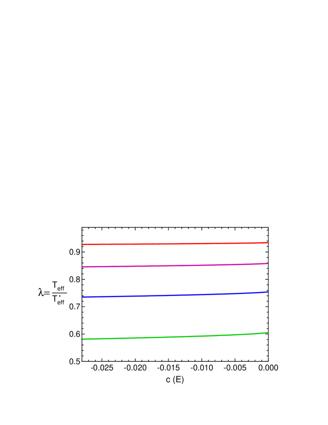
Figure 2: (Color Online) $\lambda=T_{eff}/T^{\prime}_{eff}$ as a function of $c$ in the case ${\bf m}_{p}\uparrow\downarrow{\bf e}_{z}$ for $eV=k_{B}T$ (red), $eV=5k_{B}T$ (magenta), $eV=10k_{B}T$ (blue), $eV=20k_{B}T$ (green).

We fix the Gilbert damping to $\alpha=0.01$, the ratio of anisotropies to $d=0.028$, the polarization to $P=0.81$, and $M_{s}\mathcal{V}/\gamma=10\hbar$. These values define the ratio $D_{0}/D_{th}$ as a function of $eV/k_{B}T$. The results for $\lambda={T_{eff}}/{T^{\prime}_{eff}}$ are plotted in Fig. 2. As can be seen from the plot taking into account the nonequilibrium noise results in a renormalization of the effective temperature. This renormalization is proportional to the applied voltage $V$ and can be very strong for sufficiently large values of $V$. The deviation from the purely thermal case ($\lambda=1$) approaches 15% for $eV=5k_{B}T$ and is thus experimentally not negligible! For $eV=10k_{B}T$ the deviation is even in the order of 25% and grows further with the voltage. The variation of $\lambda$ with energy is on the other hand very weak. This indicates that the influence of the angle dependence is rather small or in other words: The angle-dependence of the correlator does not lead to a significant variation of $T_{eff}$ with precession orbit.

Let us continue our discussion of the renormalized effective temperature by considering the limit where the equilibrium part of the correlator is much smaller than its nonequilibrium part and thus may be neglected. In this case we define the following quantity of interest

$${\lambda^{\prime}(E)}=\frac{D_{0}}{D_{th}}\lambda(E)\ .$$ (47)

One should note the difference between $\lambda$ and $\lambda^{\prime}$. From (44) we see that $\lambda$ is the ratio of the effective temperatures $T_{eff}$ and $T^{\prime}_{eff}$ for systems without and with nonequilibrium noise respectively. On the other, from the definition (47) it is clear that $\lambda^{\prime}$ is a measure for the influence of the angle dependence of the correlator. The stronger $\lambda^{\prime}$ deviates from $\lambda^{\prime}=1$ the stronger is the influence of the angle-dependence.

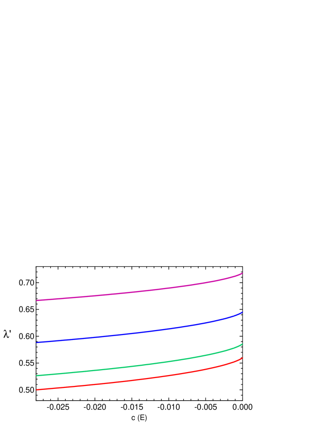
Figure 3: (Color Online) $\lambda^{\prime}$ as a function of $c$ in the case ${\bf m}_{p}\uparrow\downarrow{\bf e}_{z}$ for $P=1$ (red), $P=0.9$ (green), $P=0.7$ (blue), $P=0.5$ (magenta). $d=0.028$.

In Fig. 3 we plot $\lambda^{\prime}$ for our model system for $d=0.028$ and different values of $P$. As one can see from Fig. 3 the largest deviation from $\lambda^{\prime}(E)=1$ (corresponding to the strongest influence of the angle-dependence) is present at the minimum of the well ($c=-d=-0.028$). The smallest deviation from $\lambda^{\prime}(E)=1$ is observed for orbits which lie near the separatrice. The overall change of $\lambda^{\prime}(E)$ for $P=1$ is of the order of 10%.

These results provide a good insight into the influence of the angle-dependence. As $\lambda^{\prime}\sim 1/T^{\prime}_{eff}$, a small value of $\lambda^{\prime}$ indicates a ”hot” spot whereas large values of $\lambda^{\prime}$ correspond to ”cold” spots on the $m$-sphere. For the particular system under consideration, cf. Eq. (45), the equilibrium position of the magnetization is roughly along the $z$ axis. SW orbits of precession are symmetric with respect to this axis. At the bottom of the well $\theta=\pi$ and the spin shot noise has its maximal value. We hence expect a hot spot at the minimum of the well. With increasing energy the orbits will become larger. The angle $\theta$ will vary along these orbits. However as the orbit energy grows the trajectories increasingly go through regions of smaller $\theta$, so that the average value of $\theta$ will diminish with orbit energy. As a consequence the nonequilibrium noise will become smaller as well. Cold orbits should be hence those that are in the vicinity of the separatrice. This is exactly what can be read off from Fig. 3. Our findings are thus in agreement with the geometrical situation. Cold spots and hot spots on the $m$-sphere are shown in Fig. 4.

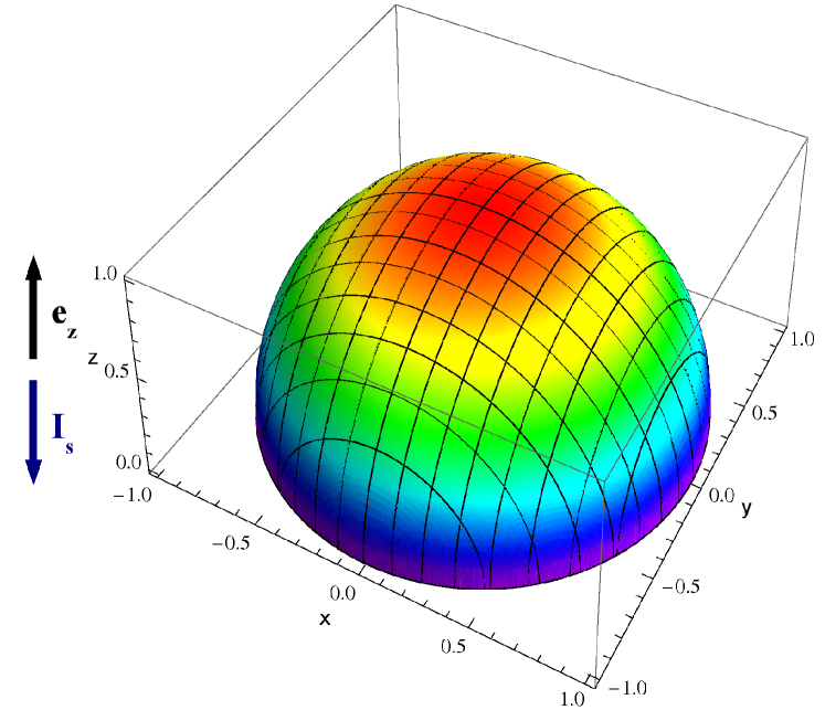
Figure 4: (Color Online) Hot spots (red) and cold spots (blue) on the $M$-half-sphere in case of ${\bf m}_{p}\uparrow\downarrow{\bf e}_{z}$. The noise intensity is highest at the bottom of the well.

IV Switching time of spin-torque structures

The switching process can be analyzed by performing numerical simulations of the Langevin equations of motion with the inclusion of temperature and shot noise via the random field term. In this section we present such simulations for Gilbert damping of $\alpha=0.01$, an anisotropy ratio of $d=0.028$, and with a spin torque current characterized by $J$ and polarized in the $\mathbf{m}_{p}=-e_{z}$ direction.

Before going further though, it would be useful to consider how the system acts in the absence of the noise. In such a case the switching occurs when the energy current (1.34) is positive for all values of energy between the starting position (say positive $z$ direction) and the saddle point. Since the probability function $\rho_{i}^{E}(E,t)$ is always positive it stand to reason that a switch will only happen if $0\leq-\alpha I_{i}^{E}(E)+J\mathbf{m}_{p}\cdot\mathbf{I}_{i}^{M}(E)$. We plot this quantity as a function of energy for various values of the spin-current $J$ in Fig. 5. From this we also gain a useful reference value for the critical current current which is $J_{c}=\frac{\alpha I_{i}^{E}(E_{sad})}{\mathbf{m}\cdot\mathbf{I}_{i}^{M}(E_{sad})}=0.00645M_{s}$. The positive value signifies the tendency towards the switching. In the first example with $J=0.77J_{c}$ the noiseless system, being driven by the dissipation towards the stable position, does not switch. It is worth noticing that in the presence of the noise the switching nevertheless does occur, but it takes exponentially long time. In the three other examples $J\geq J_{c}$ and the magnetization current is always directed towards the saddle. Therefore even the noiseless system does switch and the noise serves to introduce an uncertainty in the switching time.

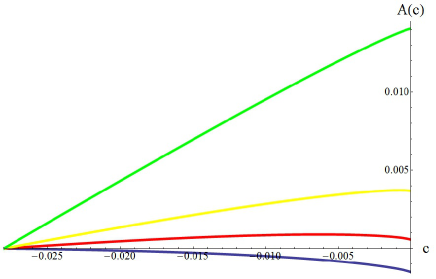
Figure 5: (Color Online) Plots $A(E)=-\frac{\alpha}{M_{s}}I_{i}^{E}(E)+\frac{J}{M_{s}}\mathbf{m}_{p}\cdot\mathbf{I}_{i}^{M}(E)$ as a function of energy $c=2E/\kappa_{2}$ over a range of spin torque current. From bottom to top: Blue = $0.77J_{c}$, Red = $1.08J_{c}$, Yellow = $1.55J_{c}$, Green = $3.10J_{c}$

Putting the thermal noise back into the system, we set the noise strength parameter to $D_{th}=0.00001\gamma M_{s}$. Simulations are then run by starting each particle at $\theta=0$, allowing it to come into thermal equilibrium with the system, turning the current on and calculating how long it takes for it to go past the saddle point into the second well. This is done for many particles for a given current value and over several different current values. A typical trajectory of the system is represented by the graph $\theta$ as a function of time in Fig. 6 for $J=1.08J_{c}$. It may be seen that it takes many revolutions before the system finally switches to the basin of attraction of the true stationary points at $t\approx 700$.

Figure 6: A typical realization of $\theta$ as a function of time (in units of $(\gamma M_{s})^{-1}$) for $J=1.08J_{c}$.

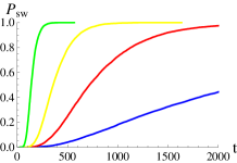
Figure 7: (Color Online) (Left) Shows the switching probability as a function of time (in units of $(\gamma M_{s})^{-1}$) for various current values. (From left to right: Green = $3.10J_{c}$, Yellow = $1.55J_{c}$, Red = $1.08J_{c}$, Blue = $0.77J_{c}$). (Right) Shows the average switching time (in units of $(\gamma M_{s})^{-1}$) as a function of $\frac{J}{J_{c}}$.

Let us estimate the contribution of the nonequilibrium noise to the switching process under realistic experimental conditions. From Eq. (26) we obtain the relationship between equilibrium noise and non-equilibrium noise

$$\frac{D_{\mathrm{neq}}}{D_{\mathrm{eq}}}=\frac{\hbar^{2}\gamma}{8ek_{B}M_{s}\mathcal{V}\alpha}\frac{I}{T}.$$ (48)

Replacing $I$ with the critical current

$$I_{c}=J_{c}\frac{4M_{s}e\mathcal{V}}{\hbar}$$ (49)

where $J_{c}$ is the minimum spin current needed to cause a switch in the absense of noise, we obtain

$$\frac{D_{\mathrm{neq}}}{D_{\mathrm{eq}}}=\frac{\hbar\gamma}{2k_{B}\alpha}\frac{J_{c}}{T}.$$ (50)

Using the material parameters in Ref. [Katine00, ], $M_{s}=1440$ emu, nanopillar volume = $1.97\times 10^{-17}cm^{3}$, and switching current $I_{c}\approx 10^{9}A/cm^{2}$, the shot noise, $D_{0}$, at the critical current is equivalent to the thermal noise, $D_{th}$, of temperature $T_{c}\approx 15$ K. Even though the theoretical switching current and the experimentally determined switching current of Ref. [Katine00, ] differ by more than an order of magnitude (such a discrepancy is mentioned in many experimental studies, including Ref. [Katine00, ]) the theoretical approach can be used to gain insight into how the shot noise at the switching current scales with the parameters of a nanopillar.

If we set $D_{0}=D_{th}$ again and include our calculation of the switching current we find $T_{c}\propto J_{c}/(\alpha P)$ where $J_{c}$ is the critical spin-torque current needed to cause a spin-flipping event (in the absence of noise) and $P$ is the degree of polarization of the current. $J_{c}$ is determined by the relative values of $H_{k}$ and $M_{s}$ and has the units of magnetization. For the simple case with only easy-axis anisotropy ($E=-\frac{1}{2}\mu_{0}H_{k}M_{s}\cos^{2}\theta$), $J_{c}=\alpha H_{k}$, and therefore $T_{c}\propto\frac{H_{k}}{P}$. Therefore for materials and/or geometry with a bigger anisotropy field the shot noise may be a dominant source of noise at temperatures well above $15K$. Moreover, in the simplest case where we only have uniaxial anisotropy and an applied external field along the easy axis it can be shown that

$$J_{c}=\alpha(H_{k}+H_{{\mathrm{ext}}}).$$ (51)

This means the relative strength of the non-equilibrium noise scales with the potential well depth of our system. By applying an external field we can increase the maximum allowed current before a switch takes place and thus increase the importance of non-equilibrium noise.

Since the initial condition is taken out of a stationary distribution (without the spin current) and subsequent evolution is subject to the Langevin noise, the time of the switching is a random quantity. The percentage of trial systems that have switched as a function of time is shown in the left panel of Fig. 7 for four different values of the spin-current. The time derivatives of these graphs provide probability distribution functions of the switching time. One may then evaluate the first moment of these distributions which gives the mean switching time for a given value of the spin current. The right panel of Fig. 7 shows such a mean switching time as a function of $J/J_{c}$. One may notice that for $J\leq J_{c}$ the switching time grows exponentially, while for $J\geq J_{c}$ the switching time becomes relatively short (although it is still substantially longer than the inverse precession frequency).

V Conclusion

We would like to conclude with the following remarks. The study of noise in dynamical magnetic systems is a broad and fascinating field. In particular, in view of potential applications of magnetic nanodevices, both equilibrium and nonequilibrium noise may play an important role. For example, the stability of magnetic storage devices is strongly influenced by thermal fluctuations. The functionality of new generation technologies (such as the magnetic random access memory (MRAM) Prinz with STT writing or the racetrack memory ParkinRacetrack ) is largely based on the spin torque phenomenon. The latter is a nonequilibrium effect and thus besides the temperature also nonequilibrium sources of noise may play an important role.

A way to introduce fluctuations into magnetization dynamics is to add a random component to the effective field or to the current in the phenomenological LLG equation. The noise is then defined by the value of its correlator (and its higher order cumulants). The determination of the noise correlator is of great importance as it defines the noise properties. In addition it may give insight into the physical context.

A powerful and very flexible tool is the Langevin approach based on the Keldysh path integral formalism. Starting from a microscopic model one derives the equations of motion for the magnetic system. Fluctuations naturally arise as a generic feature of the Keldysh approach. We have demonstrated the applicability of this method to magnetic systems on the example of spin shot noise in magnetic tunnel junctions. The spin shot noise correlator arose naturally, as a consequence of the sequential tunneling approximation, in second order in spin flip processes.

The Keldysh formalism is however not restricted to the system described above. In particular it may be used in the context of nonuniform magnetic textures (as domain walls for instance). Promising advances in this direction have already been reported DuineLucassen08 and demonstrate the versatility of the method as well as inspire us with curiosity about future developments.

Finally, to investigate the influence of the spin shot noise on spin torque switching rates we have generalized the Fokker-Planck approach of Ref[ApalkovPRB, ]. We have shown that the nonequilibrium noise manifests itself in a renormalized effective temperature. In particular at low temperatures we could observe a significant variation of the noise with orbit energy, reflecting ”cold” and ”hot” trajectories of the magnetization vector with respect to the noise intensity.

References

- [1] D. C. Ralph and M. D. Stiles. J. Magn. Magn. Mater., 320:1190, 2008.
- [2] J. C. Slonczewski. J. Magn. Magn. Mater., 286:L1, 1996.
- [3] L. Berger. Phys. Rev. B, 54:9353, 1996.
- [4] M. Tsoi, A. G. M. Jansen, J. Bass, W. C. Chiang, M. Seck, V. Tsoi, and P. Wyder. Phys. Rev. Lett., 80:4281, 1998.
- [5] E. B. Myers, D. C. Ralph, J. A. Katine, R. N. Louie, and R. A. Buhrman. Science, 285:867, 1999.
- [6] J. A. Katine, F. J. Albert, R. A. Buhrman, E. B. Myers, and D. C. Ralph. Phys. Rev. Lett., 84:3149, 2000.
- [7] M. Tsoi, A. G. M. Jansen, J. Bass, W. C. Chiang, V. Tsoi, and P. Wyder. Nature, 406:46, 2000.
- [8] S. I. Kiselev, J. C. Sankey, I. N. Krivorotov, N. C. Emley, R. J. Schoelkopf, R. A. Buhrman, and D. C. Ralph. Nature, 425:380, 2003.
- [9] W. H. Rippard, M. R. Pufall, S. Kaka, S. E. Russek, and T. J. Silva. Phys. Rev. Lett., 92:027201, 2004.
- [10] I. N. Krivorotov, N. C. Emley, J. C. Sankey, S. I. Kiselev, D. C. Ralph, and R. A. Buhrman. Science, 307:228, 2005.
- [11] W. F. Brown. Phys. Rev., 130:1677, 1963.
- [12] Z. Li and S. Zhang. Phys. Rev. B, 69:134416, 2004.
- [13] D. Cimpoesu, H. Pham, A. Stancu, and L. Spinu. J. Appl. Phys., 104:113918, 2008.
- [14] D. M. Apalkov and P. B. Visscher. Phys. Rev. B, 72:180405, 2005.
- [15] D. M. Apalkov and P. B. Visscher. J. Magn. Magn. Mater., 159:370, 2005.
- [16] J. Foros, A. Brataas, Y. Tserkovnyak, and G. E. Bauer. Phys. Rev. Lett., 95:016601, 2005.
- [17] F. J. Lazaro J. L. Garcia-Palacios. Phys. Rev. B, 58:14937, 1998.
- [18] W. Scholz, T. Schrefl, and J.Fidler. J. Magn. Magn. Mater., 233:296, 2001.
- [19] J. C. Sankey, I. N. Krivorotov, S. I. Kiselev, P. M. Braganca, N. C. Emley, R. A. Buhrman, and D. C. Ralph. Phys. Rev. B, 72:224427, 2005.
- [20] W. H. Rippard, M. R. Pufall, and S.E. Russek. Phys. Rev. B, 74:224409, 2006.
- [21] Q. Mistral et al. Appl. Phys. Lett., 88:192507, 2006.
- [22] A. L. Chudnovskiy, J. Swiebodzinski, and A. Kamenev. Phys. Rev. Lett., 101:066601, 2008.
- [23] E. B. Myers, F. J. Albert, J. C. Sankey, E. Bonet, R. A. Buhrman, and D. C. Ralph. Phys. Rev. Lett., 89:196801, 2002.
- [24] S. Urazhdin, N. O. Birge, W. P. Pratt, Jr., and J. Bass. Phys. Rev. Lett., 91:146803, 2003.
- [25] S. Urazhdin, H. Kurt, W. P. Pratt, Jr., and J. Bass. Appl. Phys. Lett., 83:114, 2003.
- [26] A. Fabian, C. Terrier, S. Serrano Guisan, X. Hoffer, M. Dubey, L. Gravier, J.-Ph. Ansermet, and J.-E. Wegrowe. Phys. Rev. Lett., 91:257209, 2003.
- [27] S. Krause, L. Berbil-Bautista, G. Herzog, M. Bode, and R. Wiesendanger. Science, 317:1537, 2007.
- [28] L. Neel. Ann. Geophys., 5:99, 1948.
- [29] T. Holstein and H. Primakoff. Phys. Rev., 58:1098, 1940.
- [30] A. Kamenev. Many-body theory of non-equilibrium systems. In Nanophysics: Coherence and Transport, pages 177–246. Elsevier, Amsterdam, 2005.
- [31] Y. Tserkovnyak, A. Brataas, and G. E. W. Bauer. Phys. Rev. Lett., 88:117601, 2002.
- [32] Y. Tserkovnyak, A. Brataas, G. E. W. Bauer, and B. I. Halperin. Rev. Mod. Phys., 77:1375, 2005.
- [33] G. A. Prinz. Science, 282:1660, 1998.
- [34] S. S. P. Parkin, M. Hayashi, and L. Thomas. Science, 320:190, 2008.
- [35] M. E. Lucassen and R. A. Duine. arXiv:0810.5232v3 [cond-mat.mes-hall], 2009.