Searchable Sky Coverage of Astronomical Observations: Footprints and Exposures

Abstract

Sky coverage is one of the most important pieces of information about astronomical observations. We discuss possible representations, and present algorithms to create and manipulate shapes consisting of generalized spherical polygons with arbitrary complexity and size on the celestial sphere. This shape specification integrates well with our Hierarchical Triangular Mesh indexing toolbox, whose performance and capabilities are enhanced by the advanced features presented here. Our portable implementation of the relevant spherical geometry routines comes with wrapper functions for database queries, which are currently being used within several scientific catalog archives including the Sloan Digital Sky Survey, the Galaxy Evolution Explorer and the Hubble Legacy Archive projects as well as the Footprint Service of the Virtual Observatory.

1. Introduction

Astronomers have to keep accurate records of where their observations are located on the sky. Beyond the direction and angular size of the field of view, we have detailed information available about the precise sky coverage derived from the exact shape of our detectors. This coverage is invaluable for most statistical studies, e.g., luminosity functions or especially analyses of spatial clustering.

The de facto standard of the Flexible Image Transport System (FITS; Wells et al., 1981) has reserved keywords for the World Coordinate System (WCS; Greisen & Calabretta, 2002) specification, and parameters that specify the transformation from image pixels to sky coordinates (and reverse), are present in the header of most FITS files. While the WCS is perfectly adequate for individual exposures, multiple observations are difficult to describe in a single system. Every field has potentially a separate coordinate system, hence moving from field to field is convoluted, and makes it cumbersome to answer even simple questions, e.g., whether two separate fields overlap.

The footprint of a large-area survey might be complicated but the small-scale irregularities are even more problematic. Not only the depth of a survey changes as a function of the position on the sky, but parts of the observations are often censored for various reasons, such as bright stars blocking the view, satellite trails, artifacts from reflections. If we would like to represent all these on the sky, we need a scalable solution that works for shapes of arbitrary complexity and size from the subpixel level to the entire sky. We need tools to create and manipulate these descriptions right there where the data are and utilize the information efficiently.

Geographic Information Systems (GIS) were designed with a similar goal in mind. There are however subtle differences, that are large enough that GIS systems are not quite applicable to astronomy directly. The modern mapping systems do not extend much beyond the basic features of projected maps but provide very efficient tools for finding nearby places and shortest routes, etc. Even the most complicated GIS shapes are limited to spherical polygons whose sides are great circles (or straight lines in the projection.) In astronomy, the approximations with such polygons would be unacceptably inaccurate or prohibitively redundant, hence there is need for an extended set of features to represent the geometries of the observations and surveys.

Some of the concepts discussed in the paper are not new and have been introduced and studied previously in different fields. Books by Samet (1989, 1990) detail the quad-trees for spatial searches that Barrett (1994) advocated using for astronomy data. Fekete & Treinish (1990); Fekete (1990); Short et al. (1995) developed an icosahedron-based methodology for Earth sciences, and Kunszt et al. (2000, 2001) introduced the convex description and the Hierarchical Triangular Mesh, a triangulation that was also used by Lee & Samet (1998) with a different numbering scheme. A similar representation of shapes is also found in Hamilton & Tegmark (2004) and Swanson et al. (2008). Goodchild et al. (1991); Goodchild & Shiren (1992) and Song, Kimerling & Sahr (2000) introduced the Discrete Global Grid for GIS systems, an equal area variant of the same triangulation idea. The integration to relational databases is discussed in Gray et al. (2004).

The goal this paper is to provide the astronomy community with a complete and consistent view of the current and much improved methodology built on a new fully functional spherical geometry framework, and describe the implementations and interfaces used in several astronomy archives and tools today including the Sloan Digital Sky Survey (Thakar et al., 2008), the Hubble Legacy Archive (Greene et al., 2007), the Galaxy Evolution Explorer and the NVO Footprint Service (Budavári et al., 2007). In Section 2 we describe how to specify spherical shapes and manipulate them. Section 3 deals with the spherical geometry of the region representations and Section 4 discusses an efficient search method based on the Hierarchical Triangular Mesh. In Section 5 we provide details of our software solution including the implementation of the database routines and their usage. Section 6 summarizes the main results, along with current and future applications in astronomy.

2. Shapes on the Celestial Sphere

In cartography, maps are typically local projections, e.g., the pages of an atlas that just overlap so that they provide enough reference for navigating a road or a trail, and in general, moving from one projection to another can be quite difficult. In astronomy, the usage pattern is different and usually more global that warrants the use of a true spherical geometry.

Spherical polygons are closed geometric figures over the sphere, formed by arcs of great circles. Generalized spherical polygons (GSPs) are similar, but their arcs can also be small circles. These are conceptually simple and yet versatile enough to represent most common shapes in astronomy. They easily describe circles, rectangles (even with curved sides), and where they cannot precisely track a boundary, an accurate approximation is possible by a short series of arc segments. Not only do they conveniently describe spherical shapes but they also provide a very compact representation. For example, the vertices and the equations of the edges (arcs) define the outline of a generalized spherical polygon, and its inside can be determined by the order of the vertices. One convention is to define the inside to be to the left as one traverses around the polygon. Either a small or a great circle can be defined as the intersection of the unit sphere with a 3-D plane. This enables us to use another, dual representation, by using half-space contraints that define the interior surface area of these spherical circles, instead of their outline. If we embed the surface of the unit sphere in a 3-dimensional Eucledian space, we can use 3D directed planar (halfspace) constraints and their boolean combinations to select parts of the sphere that represent various spherical shapes of this family describable by GSPs. Regions that cannot be represented this way would be the curves defined by intersections of higher order surfaces with the sphere, like quadrics. These two alternative descriptions are formally equivalent but have different properties that make them preferable for certain types of problems. Both have advantages and disadvantages but we do not have to choose one. In this section, we first elaborate on the surface or convex representation in detail with special emphasis on its strengths, and point out how to obtain the outline algorithmically.

2.1. Halfspaces, Convexes and Regions

Going from a two-dimensional representation of spherical shapes to a three-dimensional description provides a uniform framework with readily available geometrical concepts to build on. A halfspace is a directed plane that splits the 3-D space in two. In our context, it represents a spherical cap when intersected with the unit sphere. It is defined by a direction, i.e., a unit vector $n$, and a signed scalar offset $c$, measured along the normal vector from the origin. Using a unit-sphere centered on the origin of a Cartesian coordinate system, the parameter $c$ can take values between 1 (an infinitely small cap) and -1 (the whole sky). The value of 0 corresponds to a special case and represents half the sky cut along a great circle. In general, $c$ is the cosine of the angular radius of the cap. The caps with a negative $c$ are called holes. Another common shape in astronomy is a rectangle in the tangent plane defined by the geometry of the detector. Since a straight line in any tangent plane projects onto a great circle on the surface of the sphere, the rectangle is a convex formed by the intersection of four zero-offset halfspaces, whose normal vectors point in the direction of the neighboring vertices’ cross products.

An intersection of halfspace constraints represents a (possibly open) 3-D convex polyhedron, which in turn describes a more complicated shape when it intersects the unit sphere. Despite their simplicity in 3-D, convexes can define a large variety of spherical shapes, e.g., rings, diamonds or other polygons of “straight” or curved sides. In fact, they can even represent multiply connected shapes of arbitrarily large topological complexity. For example, the vertices and edges of a large enough cube centered on the sphere can define eight disjoint generalized spherical triangles as they poke through the surface.

Nevertheless, convexes are constrained in 3-D and, hence are limited in what types of spherical shapes can describe. More general spherical regions can be defined as the unions of convexes. This hierarchy of halfspaces, convexes and regions and their negation (or difference) provides a complete algebra over these spherical regions, enabling extreme flexibility and efficiency.

2.2. Point in a Region

One of the most common tasks is the containment test to decide whether a point is inside a region. We start with the most basic elements of the region, the halfspaces. A point (unit vector $r$) is inside a halfspace ($\mbox{\boldmath{$n$}},c$), if the dot product of the two vectors is greater than the offset,

$$\mbox{\boldmath{$n$}}\cdot\mbox{\boldmath{$r$}}>c.$$ (1)

While this is straightforward to see, its computational simplicity is striking, and has serious consequences for the performance of any implementation using this formalism. For example, the computation requires only three multiplications and one comparison for a circle and four times that for a spherical quadrangle, regardless of the size and actual shape.

Testing a point against a convex simply consists of checking whether the point is inside all its halfspaces. If yes, the point is inside; otherwise outside. As a region is the union of its convexes, it contains a point if any of its convexes contains the point.

2.3. Boolean Algebra of Regions

Within this framework, the boolean algebra of regions maps very well onto basic set operations on the collections of halfspaces and convexes. The set of regions is closed for the operations one routinely performs when deriving survey specific geometries. The same is not true for the convexes.

The union of two or more regions is a region that includes all the convexes,

$$R^{(1)}\cup R^{(2)} = C^{(1)}_{1}\cup\dots\cup C^{(1)}_{n}\cup C^{(2)}_{1}\cup\dots\cup C^{(2)}_{m}$$ (2)

$$= C_{1}\cup\dots\cup C_{n+m}=R$$ (3)

by definition. Also the intersection of two or more convexes is a convex that includes all their halfspaces,

$$C^{(1)}\cap C^{(2)} = H^{(1)}_{1}\cap\dots\cap H^{(1)}_{n}\cap H^{(2)}_{1}\cap\dots\cap H^{(2)}_{m}$$ (4)

$$= H_{1}\cap\dots\cap H_{n+m}=C$$ (5)

and, in turn, the intersection of regions is a region whose convexes are the pairwise intersections of the convexes, e.g., for two

$$R^{(1)}\cap R^{(2)}=\bigcup_{i,j}\left(C^{(1)}_{i}\cap C^{(2)}_{j}\right)$$ (6)

It is straightforward to define the differences of halfspaces, convexes, and regions, even if not as simple as the above operations. Let us first look at two halfspaces. We see that their difference is

$$H_{1}\setminus H_{2}=H_{1}\cap\bar{H}_{2}$$ (7)

where $\bar{H}$ is the negate or inverse of $H$, which is obtained by simply flipping the sign of its normal vector and the offset. Similarly, subtracting a halfspace from a convex is also simple as is the subtraction from a region. It might look logical to express the difference of two convexes as a region whose convexes are

$$C^{(1)}\setminus C^{(2)}=\bigcup_{i}\left(C^{(1)}\setminus H^{(2)}_{i}\right)=\bigcup_{i}\left(C^{(1)}\cap\bar{H}^{(2)}_{i}\right)$$ (8)

but the constructed convexes would overlap, hence the following procedure is preferred to avoid the overlaps

$$C^{(1)}\setminus C^{(2)}=\bigcup_{i}\left(C^{(1)}\cap\bar{H}^{(2)}_{i}\bigcap_{k}^{i-1}H^{(2)}_{k}\right)$$ (9)

Also we difference a region and a convex by subtracting the convex from all the convexes of the region. By substituting the all-sky coverage into $C^{1}$ of the previous equation, we get the region of a negated convex

$$\bar{C}=\bigcup_{i}^{n}\left(\bar{H}_{i}\bigcap_{k=1}^{i-1}H_{k}\right)$$ (10)

The negate of a region is in turn the intersection of its inverted convexes, by a simple application of deMorgan’s rules. From these formulas we can also see that it is not enough to stop at the level of the convexes, because even if the basic building blocks of a particular geometry are simple, subsequent operations quickly yield more complicated descriptions that can only be represented as a region.

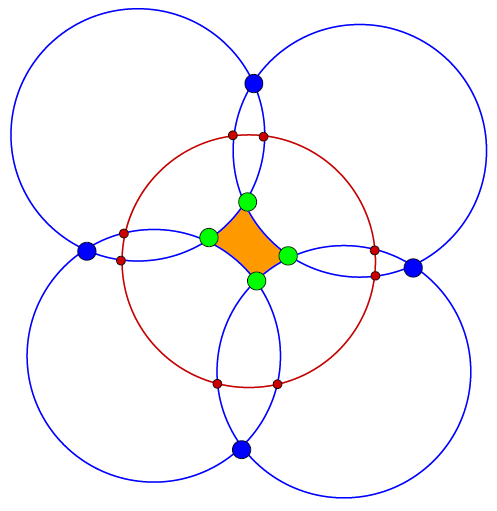
Figure 1.— The concave diamond shape is described by four halfspaces of negative offsets, whose arcs draw its outline, plus a fifth constraint that separates the diamond from the remainder of the sphere outside the four holes.

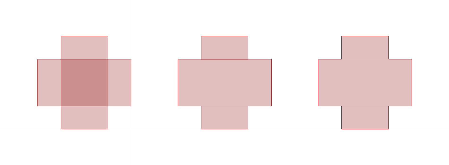
Figure 2.— The union of two overlapping rectangles (left) is turned into three disjoint convexes (middle) in the process of simplification. The outline (right) eliminates those parts of the arcs that are internal and cancel out.

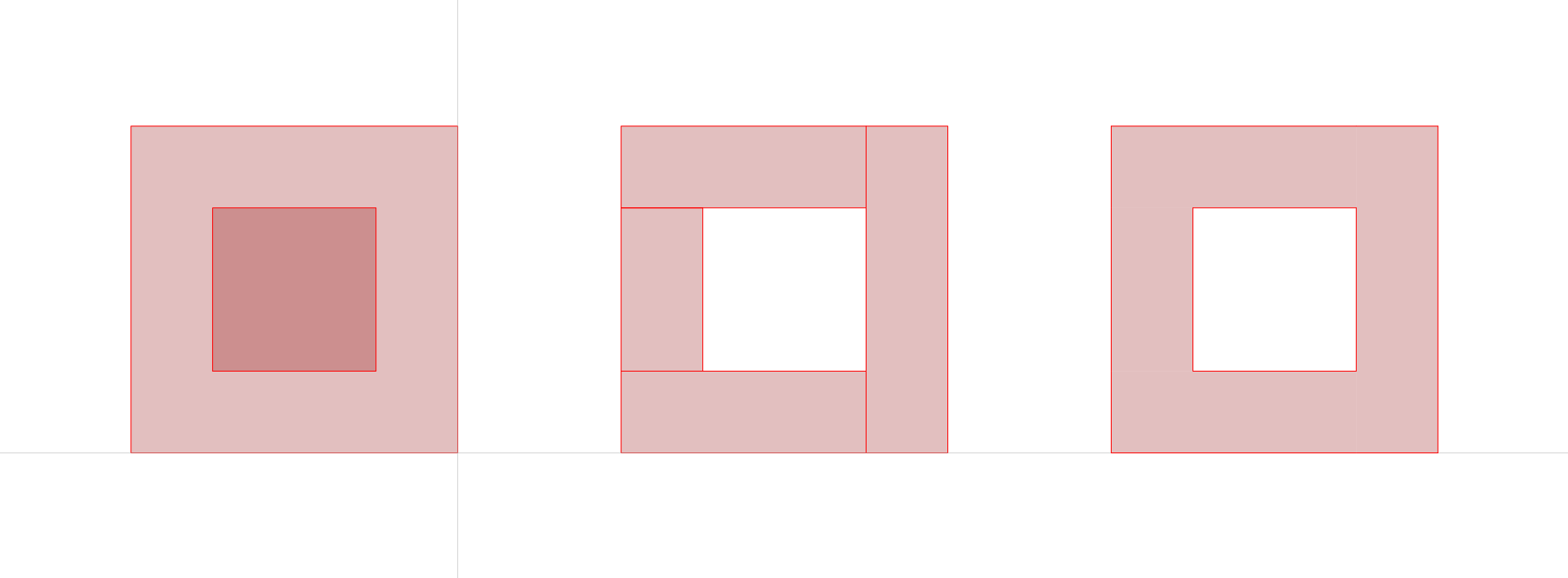
Figure 3.— The subtraction algorithm is illustrated on two rectangles (left). The difference consists of four disjoint rectangles (middle), whose outline (right) has much fewer arcs than the patches.

3. Spherical Geometry

With this elegant formalism in hand, the practical challenge is to derive irreducible representations of the results of these operations, discarding empty regions and redundant constraints. In general, this can be a compute-intensive task but, most of the time it is very fast and done as a pre-processing step that is well-worth the effort. The description not only becomes more compact but the simpler form speeds up subsequent analyses. This region simplification is the topic of this section, where one has to move beyond the basic 3-D concepts of the previous paragraphs and solve the spherical geometry of the region.

3.1. Patches and Simplified Convexes

A region is the union of convexes, so one has to start by simplifying all of its convexes individually. For many of the subsequent tasks the frequency of intersections will depend on the radii of the caps, thus it is a good practice to sort the collection by increasing size. After making sure that the smallest cap is indeed finite (if infinitely small, the convex is empty, and is eliminated), we examine the pairwise relations of the halfspaces. Based on the topology of the halfspaces, we can discard the ones that are the same as another, and those that fully contain other halfspaces. If we find halfspaces that are each other’s inverse or simply disjoint, the convex is empty.

Having done the trivial pruning of halfspaces, there might still be redundant constraints but one can only reject them by explicitely solving for the vertices and arcs of the convex. The circumference of a halfspace, a circle, would generally intersect other circles. We compute the roots (0, 1 or 2) for all possible pairs of circles, keeping track degenerate roots where multiple ($>2$) halfspaces intersect. We now collect the roots on each circle and form arcs around the circle between the roots. Some of the arcs are invisible, i.e., outside the convex, these we can ignore, and can also prune degenerate ones, if any. At this point, one can start to form a chain (linked list) of the arcs by taking one randomly and looking to match its end point with the start point of a next arc. Then we repeat adding arcs until the starting point of the first arc is reached. This singly connected part enclosed by the arcs is called a patch.

In general, a convex could have more than one patches, in which case there could be leftover arcs. With these we can repeat the previous procedure to form the remaining of the patches. In some sense, the patches are the most basic and compact elements of the convexes. We derive a minimal enclosing circle for every patch and store them with the convex. The bounding circles facilitate quick rejections in containment tests for convexes of many halfspaces, and enable faster collision or overlap detections between shapes. In the process we keep track of the halfspaces whose arcs are present in any of the patches, these are the halfspaces that we have to keep in the simplified representation. On top of these, we have to add those halfspaces that are needed to reject the roots outside the convex. This may happen in situations such as the diamond shape that is defined as the intersection of four holes. Since the surface of the sphere is a closed manifold, these four negative halfspaces could define two patches so another halfspace is needed to select the patch we want, see Figure 1. By the end of the algorithm, the convex is left with the minimum number of halfspaces that still describes the same shape.

3.2. Region Simplification

Naturally, the simplification of a region starts by processing its convexes one by one. If we know that the convexes are disjoint or not interested in the analytic area calculation, we are done. The following steps can not only provide a region description with disjoint convexes and precise areas but enable a potential performance boost from a simpler representation.

Building on the bounding circles, first an approximate collision graph is calculated, where the links note which convex (a node in the graph) might overlap with others. It is possible that some convexes simply contain others, in which case the smaller ones are redundant, and thus quickly eliminated, simplifying the collision graph.

Partial overlaps are more difficult to deal with, and here the region algebra proves (see Section 2.3) to be invaluable. To guarantee disjoint convexes, one has to look for potential collisions between two convexes and derive new ones that do not intersect. In practice, this is simply the convex subtraction, where one keeps the larger convex and substitutes the smaller one with the difference of the two. The collision graph is updated to include the new convexes that are now disjoint from the larger one. Since the new convexes present a smaller area than their progenitor, they can only collide with those that were linked to the eliminated one. We repeat this procedure until the graph has no links left. We proceed by working with the larger convexes to guarantee that those are not broken up into many small pieces. It is common for regions to have more convexes than the original description after this step, but they will be now disjoint. During this simplification process the number of collisions often grows as for every eliminated convex we introduce one or more, whose collision links are inherited and get queued for analysis.

It is worth noting that one can also eliminate convexes by stitching them. For example, two adjacent rectangles next to one another that share an arc and have neighboring halfspaces that are identical, can be substituted by a single convex. Stitching is not only a cosmetic improvement but in certain situations can make a huge impact on the performance. One example is when working with pixels that can be merged. Heuristic simplifications can make use of this feature, as we will see in Section 3.4.

3.3. The Outline of a Region

The dual halfspace-convex-region representation has many advantages as discussed before, but in certain situations a third representation, the outline, provides further new opportunities. One obvious application is visualization, when we would like to render regions projected on the sky. In Section 4 we will also look at how the outline can be used in advanced algorithms to accelerate searches for points in a region. We started by stating that the surface and shape descriptions are theoretically equivalent but in practice going from one to the other is not always straight forward. Next we discuss the outline and its derivation. Going the other way, from outline to surface representation is less convenient and not really necessary, when working primarily with halfspaces and convexes.

The patches of a region are essentially the outlines of the convexes, but not necessarily the outline of the region. For example, the outline of a region with a single convex that has only one patch consists of the patch’s arcs. This is also true if the convex has multiple patches as patches of the same convex can never touch each other at more than a point. As soon as multiple convexes are present, adjacent ones will share arcs, at least partially. We can define a segment as part of a directed arc that has a start and an end point, and there are no additional vertex point along the arc between these two. The algorithm to create an outline would just have to remove those segments from all patches that “annihilate” each other, i.e. there are two directed segments which are identical in geometry but opposite in direction. The first step is to break up each arc into unique segments, which is performed by grouping the arcs by common circles, then ordering the circle, and breaking all arcs up into distinct segments. A possible approach to identify the “canceling” segments is to look along the common circles in the collection of all patches and for every circle identify the places where two segments are opposite to one another, and hence cancel out. In this case both are removed. To preserve the relation to the original patches, which have precomputed bounding circles, we keep the structure of the outline similar to that of the region, but the arcs of the patches are replaced by smaller segments. Such representation is most advantagous but lacks the connectivity of the arcs, which requires the visualizer to draw the arcs independently lifting the pen. A continous outline is chained into a loop of the correct order by checking the start- and endpoints.

3.4. Heuristic Simplification with Igloo

When none of the above simplification methods work well, we can use hybrid techniques where we combine the advantages of pixelization with the exact geometry. Let us imagine an large area survey that takes tens of thousands of pointed observations with a circular field-of-view, so that the circles fully overlap. While the edges of the survey are rippled and need many circles to represent it accurately, the inside of the region is contigous and simple. The aforementioned simplification rules including the stitching will not be able to achieve much improvement, although there should be a simpler form. The previous algorithms would eventually also choke on a region with $\sim$50,000 convexes where every one of the convexes overlaps with 12 other. This is similar to a good approximation for the sky coverage of the Faint Images of the Radio Sky at Twenty-centimeters (FIRST; Becker, White & Helfand, 1995) survey.

If one could break up the region into small pieces that, unlike small circles, can be stitched together neatly, then one could potentially define a small number of large convexes in the middle of the region, and eliminate the union of tens of thousands of caps. The algorithm is an elegant divide-and-conquer recursion. We need a pixelization that is a hierarchical subdivision of the surface of the sphere, where the pixels are not only nicely adjacent but also share many halfspace constraints that allow for extensive merging. Such pixelization is achieved by the Igloo scheme (Crittenden, 2000). We start with a region and build a tree, e.g, using the (3:0:3) pixelization, where only those nodes are kept that collide with the region. Every Igloo pixel is a simple convex, aswe have defined this term, namely a generalized spherical triangle or a rectangle, hence the usual region operations can be directly applied. The depth-first recursion is very efficient when one records for every node of the tree the convexes of the region that it overlaps with, so that on the deeper levels of the tree with more and more nodes, less and less convexes are to be tested per each node. We typically specify the stopping criteria for building the tree by pixel size (maximum number of levels) or by the maximum number of leaf nodes. Once the tree is ready, the geometry of every leaf is examined. We subtract the colliding convexes of the region from each leaf one by one and calculate its area (see Section 3.5).

If the pixel is completely covered, we take the convex of the pixel, otherwise derive its exact shape. The merging of the pixels into larger and larger convexes is done along the tree using the full pixels only, and once the fragmentation of the region stops the pixels to grow, one can stitch the neighboring pixels, if they are on the same level.

This procedure yields the exact region with alternative internal convexes. Taking it one step further, we can also create an even simpler region by keeping the full pixels for nodes where the overlap area is large even if not completely full. For these nodes, we define another region called the mask that defines the overshoot area of the approximation. Typical footprints already have such masks to censor areas covered by bright stars, satellite trails, etc., and adding some more does not make the subsequent analyses more difficult, instead, it can significantly simplify the description of the region.

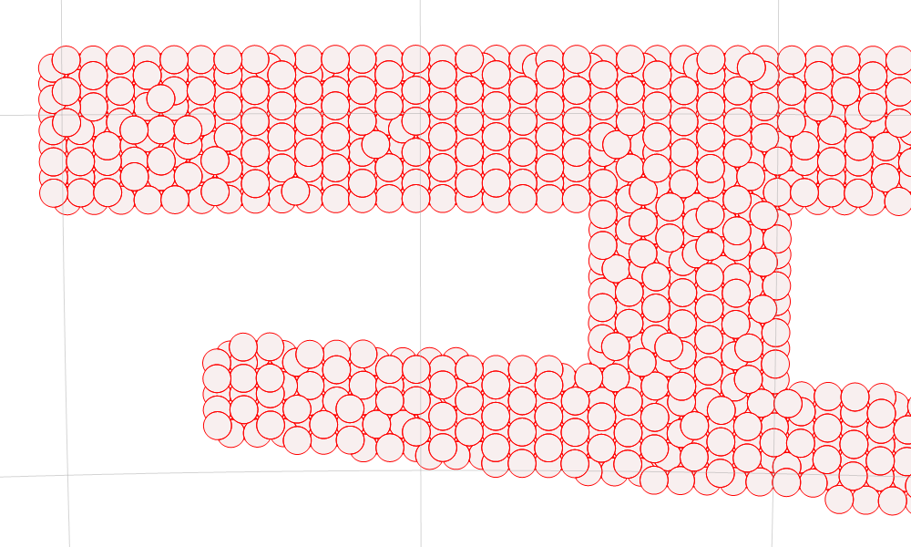
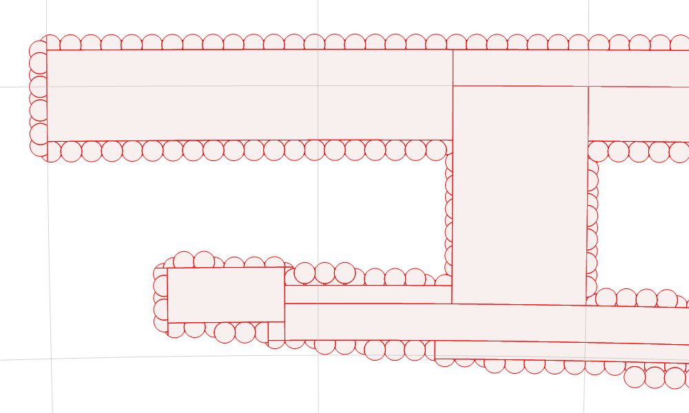
Figure 4.— Part of the FIRST footprint illustrates the power of the heuristic simplification based on a hierarchy of Igloo pixels. The brute-force method (left) runs much slower and produces many more disjoint convexes than the novel technique (right) that fills the inside of the region with stitchable convexes and merges them well.

3.5. Area Calculation

A patch is just a generalized spherical polygon bounded by small (and/or great) circles, whose arcs are ordered by design. The trick is the break a patch up into more regular pieces whose areas we can calculate. Let us pick a point arbitrarily on the sphere, e.g., at the center of mass of the vertices of a patch, and break up the polygon into spherical triangles such that one of the vertices of every triangle is this selected point and it contains an arc of the patch. Now every triangle has two great circle arcs and one of the original arcs. We follow the approach of Goodchild & Shiren (1992), by subdividing this shape into a triangle of great circle arcs and the leftover shape, known as the semilune. The area of the former is given by the Girard formula that has several variants. Here we list the one that is the most robust against degeneracy and hence should be preferred for numerical calculations over equations that appear to be simpler algebraically:

$$A_{G}=4\tan^{-1}\sqrt{z}$$ (11)

with

$$z=\tan\left(\frac{s}{2}\right)\tan\left(\frac{s\!-\!a}{2}\right)\tan\left(\frac{s\!-\!b}{2}\right)\tan\left(\frac{s\!-\!c}{2}\right)$$ (12)

where $s$ is half the circumference of the triangle with the sides $a,b,c$ in radians.

The area of a semilune is also calculated analytically but it is more convoluted. For completeness, here we print the formulas without further explanationGoodchild & Shiren (1992).

$$A_{S}=a-b\cos\theta$$ (13)

where $\theta$ is the half angle of the small circle, i.e., the radius of the cap, and

$$a = 2\arcsin\left(\tan\left(\arcsin r\right)\big{/}\tan\theta\right)$$ (14)

$$b = 2\arcsin(r\,/\sin\theta)$$ (15)

with $r$ being half the Eucledian distance between the end points of the arc. The situation is slightly complicated by the fact that certain patches are actually holes (for $\cos\theta<0$), whose area is propagated with a negative sign to obtain the correct total sum for the region.

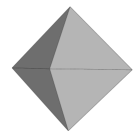
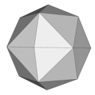
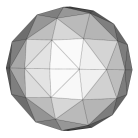
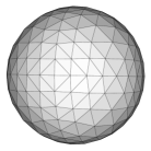
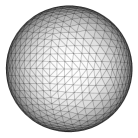
Figure 5.— The recursive subdivision of the octahedron, illustrated above, is at the heart of the Hierarchical Triangular Mesh, also known as the HTM.

4. The Hierarchical Triangular Mesh

Another pixelization of the sphere in combination with the region representation enables fast spatial searches for catalog entries of stars, galaxies and other astronomical sources that are within a spherical region on the sky. The idea is to apply a coarse filter to the entire dataset and to reject most of the sources that are outside the search region, and perform the computationally more expensive geometry test on a much smaller subset of candidates that already passed the filter.

Our choice for such a filter is based the Hierarchical Triangular Mesh, also known as the HTM (Kunszt et al., 2000). Next we discuss the properties and features of the HTM, then introduce the algorithms for creating efficient coarse filters for regions that map very well onto the indexing facilities of currently available relational database engines.

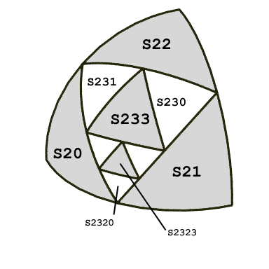
Figure 6.— The naming of the hierarchical trixels provides unique identifiers. The ensemble of all trixels at a given level can be thought of as a space-filling curve on the surface of the sphere.

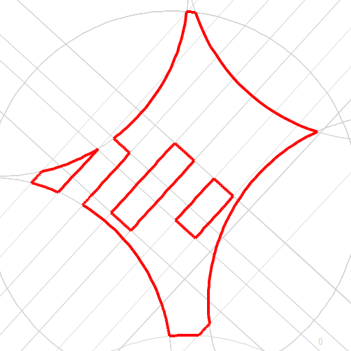
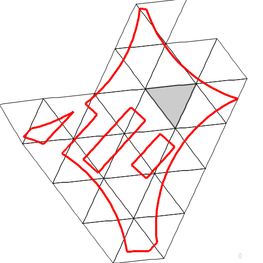
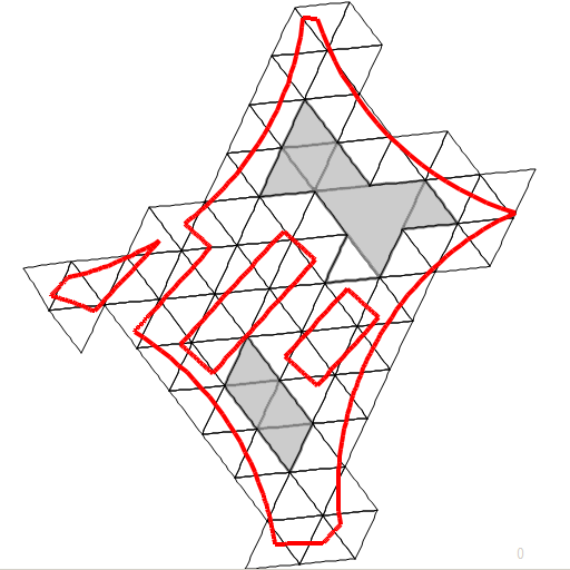
Figure 7.— A sample region from the SDSS geometry illustrates the various spherical concepts: (from left to right) (1) Circles of all halfspace contraints of the region. (2) The outline as used in the HTM algorithm. (3) The inner (filled gray) and outer covers (open triangles) of the region using larger and (4) smaller trixels.

4.1. Address of a Point

We can paint the sphere with triangular pixels that we call trixels defined by the HTM. The top nodes are the 8 faces defined by an octahedron projected onto the sphere. The children of each node are obtained by subdividing the existing triangular nodes into 4 new triangles. The sub-triangles have the current corners and the current arc’s midpoints as their corners. Finer detail is created as new levels are added by repeating the process for each triangle. In the limit, the recursive subdivision approaches the ideal sphere as in Figure 5.

All the triangles at any level have a unique identifier or trixel ID. It is an integer number, that encodes the position of the trixel in the hierarchy and is composed through the following recursive algorithm. The level 0 trixels are the faces of the octahedron. We name them with N0, N1, N2, N3 and S0, S1, S2, S3 where N and S refer to the northern and southern hemispheres, respectively. In the recursion, each triangle has four offsprings that are named by appending the index 0, 1, 2 or 3 to the parent’s name. Figure 6 illustrates the naming convention in the subdivision on a few examples.

To keep things consistent, we introduce a straightforward mapping between the name and the ID of a trixel. The ID is a 64-bit integer and is more compact than the human-readable name that can be up to 25 bytes long. First we assign the bits 11 to N and 10 to S and convert the trixel’s number betwen 0 and 3 to binary (00 and 11) and append it to the previous bits. We repeat until the desired level is reached. For example, the trixel named S2320 will convert to binary 1010111000 or decimal 696. The longer the name of a trixel, the deeper it is in the hierarchy. For practical purposes, we stop at level 20, approximately corresponding to a positional accuracy of about 0.3”. This special level-20 trixel ID is called the HtmID in our system. A 64-bit integer can hold a trixel number to level 30, although the standard IEEE-float double precision breaks down after level 25 where the positional accuracy would be about one hundredth of an arcsecond. A property of the trixel ID numbers is that the descendants of a trixel have IDs that form a consecutive list of numbers. For example, the 4 children of S2320, namely the set of {S23200, S23201, S23202, S23203}, form the range of numbers 2784–2787. The level 20 offsprings of the same trixel form the HtmID range 11957188952064–11974368821247. This is important, because we can represent any level trixel with either a single number, or with a pair of low-high HtmID values. The consequence of using the latter representation is that regions with variable size trixels can be expressed uniformly, and because the numbering provides partial coherence of the HtmID numbers.

Since trixels partition the sphere, any location is inside exaclty one trixel, so a level 20 trixel ID, or the HtmID is a fairly accurate approximation of the position. This property is exploited in our spatial search algorithm detailed in the subsequent paragraphs.

4.2. Approximate Region Covers

Simply put, a cover is a set of trixels that fully covers a region. It is an approximation of the shape by the union of a set of spherical triangles. Given a region, the algorithm starts with the eight level-0 trixels that make up the entire globe. The S2 in Figure 6 is one of these eight trixels that are initially marked as unprocessed. In the recursion, all unprocessed trixels are analyzed and get marked with one of three possible tags. The inner trixels are fully inside the region, the reject ones are completely outside and partial trixels are on the outline. Dealing with inner and reject trixels is easy. Inner trixels are saved for output, and the rejects are discarded from further consideration. A partial trixel is subdivided into four smaller trixels which are placed at the back of the unprocessed list. Eventually all trixels are tagged to the desired level of detail.

Often it is very useful to have an approximation of the inside of the region that does not touch the outline. Sources in the inner cover are guaranteed to be inside the region, hence do not require extra geometry tests. This inner cover is the union of all the inner trixels, while the aforementioned outer cover is the union of the inner and partial trixels. In fact, it is possible to obtain both sets at the same time without much extra processing. As to where to stop, there is no universal optimum, and the answer will depend on the actual dataset and region, as well as the implementation of the search engine and even its hardware configuration. Fortunately, sensible heuristics exist and the performance of the searches are considerably better than the naive implementation for any reasonable cover shapes.

4.3. Searching with HTM

Let us now examine how spatial searching is performed using an HTM cover. Assume that every source of our dataset has a pre-computed HtmID that constrains its location on the celestial sphere to within a particular level-20 trixel. The outside cover of the region can be represented as a set of HtmID intervals. If the sources are ordered by their HtmID, fetching sources in these intervals is extremely fast. If the dataset resides on disk, which is the case for any massive live astronomical catalog, getting sources in an interval consists of reading sequentially from the hard drive. At the end of every interval, the disk head is raised and re-positioned to the beginning of the next interval. This seek-time is the source of the penalty one would pay for a very accurate cover that is represented by many short intervals. Often a couple of dozen HTM ranges provide accurate representations that select a small enough candidate list with which modern CPUs can keep up with processing the exact geometry calculations. In general, any custom stopping criterion can be utilized, e.g., based on elapsed time or resolution size. One particularly interesting possibility is to monitor the area of the inner and outer covers and stop at a desired limit on their ratio. In fact, the area ratio can be approximated by the ratio of the number trixels in the two covers. The areas of trixels on the same level vary less than about 40% but the collections of (random) trixels would average out this variance to a more precise estimation of the area ratio.

5. Software Packages

Our design of the software implementation was driven by several requirements. It needed to be architecture and operating-system independent that also integrates well with the relational database technology, which is at the core of most modern astronomy archives today. We chose to build our solution in the .NET Framework programming model that satisfies our development, maintainance, portability and performance requirements. Such managed code runs in a virtual machine called the Common Language Runtime, or CLR for short. In addition to Microsoft’s CLR implementation of the Common Language Infrastructure (CLI), there is also an open-source cross-platform runtime by the Mono Project. The .NET Framework is not only OS independent but also allows for development in several programming languages and the integration of projects in a mixture of languages. Using the C# programming language, we built a set of class libraries that depend on each other, so that applications in any one of the supported languages can choose to include the appropriate modules selectively.

5.1. The Spherical Library

The basic module or assembly contains the routines to deal with the spherical geometry. Generic container classes are used to store the collection of halfspaces in a convex and the collection of convexes that make up a region. Thus managing a shape is as simple as working with lists. Here we show the C# listings of a trivial example with a convex of two halfspaces to illustrate the simplicity of the coding. First, we define the centers of the caps using J2000 (R.A., Dec.) coordinates,

Cartesian p1 = new Cartesian(180, 0);
Cartesian p2 = new Cartesian(181, 0);

then set the radius of the caps and create the halfspaces using the centers

double theta = Math.PI / 180;    // 1 degree radii
Halfspace h1 = new Halfspace(p1, Math.Cos(theta));
Halfspace h2 = new Halfspace(p2, Math.Cos(theta));

The convex is a collection of halfspaces that are added one by one after which we invoke the simplification of the description that also derives the arcs and patches of the shape along with its analytic area in square degrees.

Convex c = new Convex();
c.Add(h1);
c.Add(h2);
c.Simplify();
Console.Out.WriteLine(c.Area);

Similary a region is created by adding convexes to its collection.

Region r = new Region();
r.Add(c1);
r.Add(c2);
r.Simplify();
Console.Out.WriteLine(r.Area);

Naturally, the number of convexes in a region and halfspaces in a convex are not limited to two (and can also be one), they are only bound by system memory and computational power for processing.

Boolean operations on the shapes are implemented to perform the computations in place whereever possible. For example, the union of regions or the intersection of convexes can be done within the instance on which the method is called, but the difference of two convexes or regions is implemented to return the resulting region. On top of the straightforward translations of the algorithms in Section sec:alg, most operations have a smart version for simplified shapes. One of the advantages of using these methods is the speedup for complicated shapes, where the precomputed bounding circles reduce the computational costs. The other benefit is potentially even greater. E.g, the union of simplified regions can be done based on the assumption that the convexes of the regions are already disjoint, and hence, check for collisions among the mixed pairs only. In code, the snipets

r.Union(r2);      // regions may not be simplified
r.Simplify();     // simplification from scratch
Console.Out.WriteLine(r.Area);

and

r.SmartUnion(r2); // both simplified
Console.Out.WriteLine(r.Area);

are conceptually identical but the latter can take significanly less time as it can assume the arguments to be in the canonical form.

The application programming interface (API) supports many more advanced ways to create and manipulate regions of arbitrary complexity, the working code snipets above are here to serve as guide.

5.2. Numerical Imprecisions

Numerical stability of the implementation of the spherical algorithms is crucial and has not been easily achieved. Computations with floating-point numbers make errors that can accumulate in a series of operations. These uncertainties can result in erroneous determination of topological relations of points and planes, convexes and regions. One possible solution is not to use floating-point arithmetics. Software packages exist that work with rational numbers, and represent them as a pair of integers: the numerator and the denominator. In this setting, the values are always precise but there is an efficiency penalty. In spherical geometry, there is an even more severe problem with this approach. The set of rational numbers is not closed for operations that one has to routinely perform, e.g., the square root of a rational number can be irrational.

We use IEEE Standard 754 double-precision floating-point numbers in our implementations that most modern CPUs can efficiently process, and we carefully analyze the code for numerical stability and rounding problems. It is a surprisingly hard task. For decades, linear algebra routines, e.g., those in LAPACK, have been strengthened and optimized by hand because no generic solution exists; only best practices. Classic examples include the robust solution to the quadratic equation, or evaluating the values of $a^{2}\!-\!b^{2}$ and $\log(1+x)$. To illustrate the importance, here we describe real-life problems that make the spherical geometry computations more difficult than expected, and explain our solutions briefly. The details of error propagation in floating-point arithmetics is beyond the scope of this writing. Rather, we refer the interested reader to Goldberg (1991).

Previously we said that deciding whether a point is inside a halfspace, the most basic containment test discussed in Section 2, involves calculating the dot product of the point’s unit vector and the direction of the plane and comparing the result to the halfspace’s offset, the cosine of the cap’s radius. The numerical imprecision on the result translates to larger errors in the radius because the cosine function is quadratic at values near zero, hence using the sine can be more advantageous. Even then, when the point is very close to the plane, it is essentially impossible to decide which side it is on or whether it is contained in the plane. We circumvent the problem by not trying to answer in or out but allow for an undetermined value within a margin derived from the limitations of the representation of floating-point numbers. This value is deep in the core of routines establishing the spatial topological relations of the shapes.

Another, more subtle, algorithmic problem is the solution of the intersection of two planes, and the derivation of the intersecting points of two circles on the unit-sphere. As discussed in detail by Príamos (1992), an elegant robust solution (out of many possible derivations) is based on optimizing for the errors made in the computation of a point that the line crosses. The idea is to pick one of the x-y, y-z and x-z planes that is most perpendicular to the direction of the line, and solve for the point in that plane. This way one of the coordinates is readily fixed to be 0, and we only have to solve a 2-D linear equation for the other coordinates.

Halfspaces and vertices of spherical polygons become degenerate very frequently as a result of routine operations while building up the geometric description of observations. Without controlled accuracy these degeneracies could not be spotted and caught to derive correct representations or the regions.

5.3. Modules for HTM

Classes and routines of the HTM implementation are divided into two basic categories. The creation of the hierarchy of triangles is a module of its own. The tree is usually not created for its extremely large size but computed on the fly. Once the algorithm is fixed, the hierarchical trixels exists without the actual tree in memory or disk. The methods provide the recursion and the basic geometrical description of the pixels. For example, a single call yields the HtmID,

Cartesian p = new Cartesian(180,0); // Point on the sky
Int64 htmID = Trixel.CartesianToHid20(c); // and its ID

and another the trixel’s geometry,

Cartesian v1, v2, v3;   // Vertices of the trixel
Trixel.ToTriangle(htmID, out v1, out v2, out v3);

On top of the core module is a set of classes that deal with the regions and their topological relations to the trixels. Our efficient implementation of the HTM makes use of the internal structure of the region, and the derived properties of its convexes and patches as well as the outline. In the API, all the complexity is hidden behind simple

List<Int64> trixels = Cover.HidList(region);
Console.Out.WriteLine(trixels.Count);

Alternatively one can explicitly instantiate a cover object, and investigate the properties during processing

Cover k = new Cover(region);
k.Run();  // Default processing and stopping
          // Call k.Step() for more control
List<Int64> inner = k.GetTrixels(Markup.Inner);
List<Int64> outer = k.GetTrixels(Markup.Outer);
List<Int64> partl = k.GetTrixels(Markup.Partial);

Similarly the intervals are retrieved by a single method call and print in the following example.

List<Int64Pair> ranges = Cover.HidRange(region);
foreach (Int64Pair p in ranges)
    Console.WriteLine(p)

As shown in the examples above the HTM and Spherical Library classes and routines work together seemlessly by design. They leverage all the information available to perform the operations as fast as possible, while keeping the usage patterns simple. Under these high-level routines, powerful methods provide easy customization of the code for other type of problems and applications. One such example is the NVO’s Footprint Service that uses high-resolution HTM ranges to look for overlapping footprint, or regions that contain a given point.

5.4. Region in a String

Our basic internal string representation of the regions follows the simple structure of the collections. We enumerate the convexes and all their halfspaces

REGION
    CONVEX CARTESIAN x1 y1 z1 c1
           ...
           CARTESIAN xN yN zN cN
    CONVEX ...

with arbitrary whitespace and linefeed characters. The cartesian coordinates are the usual transformations of the J2000 $(\alpha,\delta)$ by equations

$$x = \cos\delta\,\cos\alpha$$ (16)

$$y = \cos\delta\,\sin\alpha$$ (17)

$$z = \sin\delta$$ (18)

On top of this simple description, the interfaces also support more advanced concepts via region parser based on our grammar in the Backus–Naur Form (BNF). The use of these constructs are often more straighforward than spelling out the $(x,y,z)$ coordinates of the normal vectors. Here we show the case for a couple of simple convexes often used by astronomers. The region describes the union of a circle with a radius of $60^{\prime}$ around the center at $(\alpha,\delta)=(180^{\circ},0^{\circ})$ in the J2000 coordinate system and a great-circle polygon specified by its ordered vertecies given by the angles.

REGION
    POLY J2000 180 0 182 0 182 2 180 2
    CIRCLE J2000 180 0 60

The polygon can be built up by any number of vertices (greater than two) and the region can have any combination of convex constructs. Another useful feature is the convex hull of a point set that is specified by the keyword CHULL. To specify cartesian coordinates, one can replace the J2000 keyword with CARTERSIAN and enumerate the components of the unit vector instead of the anglular coordinates.

5.5. SQL Routines

One of the most attractive advantages of developing in the .NET programming model is the elegant integration with SQL Server since the 2005 Version. The runtime is actually hosted inside the engine, which allows for the customization of the database to satisfy the astronomy specific requirements. The custom assemblies can be loaded to be part of the database along with the catalog data, and User-Defined Functions (UDFs) can wrap the functionality of the managed code that are invoked efficiently from SQL at query time. This way custom programs can run inside the database right there where the data are, and perform analyses without moving the bits on the network or even outside the SQL engine.

Our harness for the spherical implementation is schema-independent by design. This means that the same SQL routines can be present and be used in any astronomy science archive regardless of the layout of the database or the content of the tables. In fact, it is currently in use in a wide variety of services, including the Sloan Digital Sky Survey, the Galaxy Evolution Explorer and the Hubble Legacy Archive, being integrated with the Spitzer and Chandra servers, among others.

The regions are serialized into a compact binary format that contains both the halfspace-convex-region representation and the patches along with their minimal enclosing circles. The simplest way to create a region is by using the internal specification language that can describe any region but the operations are also supported when starting with basic building blocks. For example, the union of a 60’ radius circle and the spherical rectangle can be coded as follows.

DECLARE @s VARCHAR(MAX), @r VARBINARY(MAX),
        @z VARCHAR(MAX), @u VARBINARY(MAX)
SELECT @s = ’REGION CIRCLE J2000 180 0 60’,
       @z = ’POLY J2000  180 0  182 0  182 2  180 2’,
       @r = sph.fSimplifyString(@s),
       @u = sph.fUnion(@r,sph.fSimplifyString(@z))
SELECT sph.fGetArea(@r), SELECT sph.fGetArea(@u)
GO
-- 3.14151290574491  6.35572804450646

In SQL, the binary blobs of arbitrary size (up to 2GB) are represented as VARBINARY(MAX), and here we use variables of that type. Naturally, one can also create tables with VARBINARY columns to save the resulting regions within SQL Server. We note that previous version of the SQL harness, e.g., currently deployed in the SDSS Catalog Archive Server, do not use the separate sph schema but instead keep the UDFs in the default dbo using an Sph prefix, e.g., in dbo.fSphGetArea(@r).

The HTM routines in SQL provide high-performance spatial searches in combination with the builtin indexing mechanism. Scalar-valued UDFs can compute the address of a point at the default level of 20. Here we list a simple example that updates a table called PhotoObj to set the HtmID column for all rows based on their J2000 coordinates

UPDATE PhotoObj SET HtmID = dbo.fHtmEq(RA,Dec)

Using spherical regions to search for sources is also very straightforward and very efficient. In the following snippet we fetch only the rows that are in the HTM cover, hence are probably contained in the region:

WITH Cover AS
(
    SELECT * FROM dbo.fHtmCoverRegion
          (’REGION CIRCLE J2000 180 0 10’)
)
SELECT o.ObjID
FROM PhotoObj AS o INNER JOIN Cover AS c
    ON o.HtmID BETWEEN c.HtmIDStart AND c.HtmIDEnd
GO

The UDF returns a table of the HTM ranges of the approximation of the specified shape that overshoots, and the join returns instantly all the possible rows. In a real-life search, the WHERE clause of the query would have a separate containment test with the region geometry. The sole purpose of the HTM cover is to fetch the good candidates only from the disk, and it does this very fast.

5.6. The Astronomical Data Query Language

As part of the current standardization efforts of the International Virtual Observatory Alliance (IVOA), the Space-Time Coordinate metadata (STC) provides an alternative to accurately describing shapes on the celestial sphere. An STC region has both XML (STC-X) and string (STC-S) serializations that are well mapped onto our data structures, and translators are being implemented to support them. The STC-X parser is deployed and being tested as part of the the National Virtual Observatory’s (NVO) Footprint Service and the STC-S capabilities shall be part of future releases of our software packages and the service. The plain string representation STC-S is very straightforward by default. The union of a set of convexes looks like

Union J2000
(
    Convex   1 0 0   0.1
            -1 0 0  -0.5
    Convex   0 1 0   0.0
)

The simplicity of the representation comes from the defaults that are substituted automatically for the missing STC elements but it is also possible to be explicit about every detail and even have different coordinate systems for the components, e.g., in

Union
(
    Polygon FK5 J2000  180 0  182 0  182 2  180 2
    Circle  FK4 B1950  179 0  2
)

In addition to the union, STC sports a large set of features that also include intersection, difference and negation of any of the shapes.

The IVOA also working toward a standardized search language called the Astronomical Data Query Language (ADQL), which is an IVOA Recommendation as of this writing. ADQL is an extended subset of the ANSI SQL-92 standard, which adds geometrical constraints via simplified GIS-like functions (e.g., circle) and the full support of aforementioned STC representation. Building on our legacy SQL routines that currently work with the internal string representation, we are now creating new versions that input STC-S, and are designing an efficient implemention that supports the full ADQL.

6. Summmary

We explored the properties of generalized spherical polygons. We found the convex representation to be very compact and efficient. The boolean region operations are straightforward within this framework but inevitably create convoluted and redundant descriptions. The simplification involves solving the spherical geometry of the region. In the process, we summarized how to analytically calculate the areas and create the outlines of the regions.

Pixelization schemes also significantly benefit from the better representation. An optimal set of HTM triangles can be computed to cover entirely a region, or just to approximate the inside, in much less time than before. We introduced a heuristic hybrid solutions for simplifications based on the Igloo pixelization hierarchy that can tackle massive geometries where the brute-force method fails to deliver.

Our portable implementation in the .NET programming model is available for developers on the projects website. Its design enables quick development of new applications and a clean and easy integration with the SQL Server database engine that hosts several science archives today. The provided working examples illustrate common search patterns in C# and SQL. Future works include more algorithmic optimizations and full support of the IVOA’s STC and ADQL standards.

References

- Barrett (1994) Barrett, P. 1994, ADASS IV, ASP Conf. Ser., Eds: R.A. Shaw, H.E. Payne and J.J.E. Hayes, Vol. 77, 472
- Becker, White & Helfand (1995) Becker, R. H., White, R. L., & Helfand, D. J. 1995, ApJ, 450, 559
- Budavári et al. (2007) Budavári, T., Dobos, L., Szalay, A. S., Greene, G., Gray, J., & Rots, A. H. 2007, Astronomical Data Analysis Software and Systems XVI, 376, 559
- Crittenden (2000) Crittenden, R. G. 2000, Astrophysical Letters Communications, 37, 377
- Fay (2009) Fay, J. 2009. The WorldWide Telescope Manual, http://research.microsoft.com/en-us/um/people/dinos/spheretoaster.pdf
- Fekete & Treinish (1990) Fekete, G., and Treinish, L. 1990, ”Sphere quadtrees” SPIE, Extracting Meaning from Complex DAta: Processing, Display, Interaction 1259: 242-253
- Fekete (1990) Fekete, G. 1990, Rendering and managing spherical data with sphere quadtrees. Proceedings of Visualization ‘90. IEEE Computer Society, Los Alamitos, CA pp 176-186
- Goodchild et al. (1991) Goodchild, M. F., Shiren, Y., et al. 1991, ”Spatial data representation and basic operations on triangular hierarchical data structure.” National Center for Geographic Information and Analysis: Santa Barbara. Technical Report 91-8
- Goodchild & Shiren (1992) Goodchild, M. F., and Shiren, Y. 1992, A Hierarchical Data Structure for Global Geographic Information Systems , CVGIP: Graphical Models and Image Processing, 54, 31-44.
- Goldberg (1991) Goldberg, D. 1991, What Every Computer Scientist Should Know About Floating-Point Arithmetic in Computing Surveys, Association for Computing Machinery, Inc., http://docs.sun.com/source/806-3568/ncg_goldberg.html
- Gray et al. (2004) Gray, J., Szalay, A. S. Fekete, G., Nieto-Santisteban, M. A., O Mullane, W., Thakar, A. R., Heber, G., & Rots, A. H. 2004, Microsoft Research Technical Report, MSR-TR-2004-32
- Gray et al. (2006) Gray, J., Nieto-Santisteban, M. A., & Szalay, A. S. 2006, Microsoft Research Technical Report, MSR-TR-2006-52
- Gray et al. (2007) Gray, J., Szalay, A. S., Budavári, T., Lupton, R., Nieto-Santisteban, M., & Thakar, A. 2007, arXiv:cs/0701172
- Greene et al. (2007) Greene, G., Lubow, S., Budavári, T.,& Szalay, A. 2007, Astronomical Data Analysis Software and Systems XVI, 376, 193
- Greisen & Calabretta (2002) Greisen, E. W., Calabretta, M. R. 2002, A&A, 395, 1061
- Hamilton & Tegmark (2004) Hamilton, A. J. S., Tegmark, M., 2004, MNRAS, 349, 115
- Heinis et al. (2009) Heinis, S., et al. 2009, ApJ, 698, 1838
- Kunszt et al. (2000) Kunszt, P. Z., Szalay, A. S., Csabai, I., and Thakar, A. R. 2000, ‘The Indexing of the SDSS Science Archive’, In ASP Conf. Ser., Astronomical Data Analysis Software and Systems IX, eds. N. Manset, C. Veillet, D. Crabtree, Vol. 216,141.
- Kunszt et al. (2001) Kunszt, P. Z., Szalay, A. S., Thakar, A. R. 2001, in Mining the Sky: Proceedings of the MPA/ESO/MPE Workshop Held at Garching, Germany, July 31 - August 4, 2000, ESO ASTROPHYSICS SYMPOSIA. ISBN 3-540-42468-7. Edited by A.J. Banday, S. Zaroubi, and M. Bartelmann. Springer-Verlag, p. 631
- Lee & Samet (1998) Lee, M., Samet, H. 1998, Navigating through triangle meshes implemented as linear quadtrees, Technical Report 3900, Department of Computer Science, University of Maryland, April 1998
- Príamos (1992) Príamos, G. 1992, Plane-to-Plane Intersection in Graphics Gems III (ed. D. Kirk), Elsevier Science, p.233-235, p.519-520
- Samet (1989) Samet, H. 1989, The design and analysis of spatial data structres, Addison Wesley
- Samet (1990) Samet, H. 1990, Application of spatial data structures, Addison Wesley
- Short et al. (1995) Short, N.M., Cromp, R. F., Campbell, W. J., Tilton, J. C., LeMoigne, J., Fekete, G., Netanyahu, N. S., Wichmann, K., Ligon, W. B. 1995, ”Mission to Plane Earth: AI Views the World”, IEEE Expert, June, 1995, pp 24-34
- Song, Kimerling & Sahr (2000) Song, L., Kimerling, A. J., and Sahr, K. 2000, Developing an Equal Area Global Grid by Small Circle Subdivision , Proc. International Conference on Discrete Global Grids, Santa Barbara, CA, March 26-28, 2000.
- Swanson et al. (2008) Swanson, et al., 2008, MNRAS, 387, 1391
- Szalay et al. (2005) Szalay, A. S., Gray, J., Fekete, G., Kunszt, P., Kukol, P., & Thakar, A. R. 2005, Microsoft Research Technical Report, MSR-TR-2005-123
- Thakar et al. (2008) Thakar, A.R., Szalay, A.S., Fekete, G., and Gray, J. 2008: The Catalog Archive Server Database Management System , Computing in Science and Engineering, 10, 1 (Jan/Feb 2008), 30.
- Wells et al. (1981) Wells, D. C., Greisen, E. W., & Harten, R. H. 1981, A&AS, 44, 363