The $1/N$ Expansion in Noncommutative Quantum Mechanics

Abstract

We study the $1/N$ expansion in noncommutative quantum mechanics for the anharmonic and Coulombian potentials. The expansion for the anharmonic oscillator presented good convergence properties, but for the Coulombian potential, we found a divergent large $N$ expansion when using the usual noncommutative generalization of the potential. We proposed a modified version of the noncommutative Coulombian potential which provides a well-behaved $1/N$ expansion.

I Introduction

The so called $1/N$ expansion was proposed in 1974 tHooft as a scheme to nonperturbatively study QCD in the strong coupling region. In that context, calculations using a large $N$ expansion for the group $SU(N)$ have been shown to provide results with good agreement with experimental data for the $SU(3)$ chromodynamics (see manohar for a review). Since then, the $1/N$-expansion was used as an approximation method which generally gives very accurate results and can be applied to different fields, including atomic and particle physics. For massless two dimensional models where severe $IR$ divergences prevent the use of perturbation methods, the $1/N$-expansion allows to uncover very interesting peculiarities as dynamical mass generation, dynamical generation of gauge bosons, confinement and so on coleman . Other applications include studies of Bose-Einstein condensation, stochastic quantization, and noncommutative quantum field theories BoseEinsteinCondensate ; cpn ; Foerster ; grossneveu ; MGomes ; MGomes2 , to name a few. Recently, the large $N$ limit has become fundamental in the study of the Maldacena conjecture Maldacena , which allows one to obtain nonperturbative information on conformaly invariant quantum field theories.

The $1/N$-expansion has also been used in Quantum Mechanics for a large class of potentials, since it produces good results for the determination of the ground and low excited states energies. The $1/N$-expansion can be used even when the Hamiltonian cannot be separated in a solvable part plus a small perturbation; besides that fact, finding energies and wave functions is achieved by solving iterated algebraic equations, instead of solving a differential equation. This iterated procedure can be neatly implemented in any CAS (Computer Algebra System) for example.

In this paper, we are interested in the application of the $1/N$ expansion in the context of noncommutative quantum mechanical models. There has been a lot of interest in the last decades in studying theories defined over a spacetime where coordinates do not commute, in part following the discovery of noncommutative gauge theories as a low energy limit of the string theory in certain backgrounds SW . The general motivation for spacetime noncommutativity is the idea that, in distances of the order of the Planck length, the measurement of the coordinates loses all its sense due to the production of intense gravitational fields. For this reason, the usual concept of a point can not be adopted and this suggests the use of position operators that do not commute Doplicher .

These motivations rendered to noncommutative spaces a wide variety of theoretical applications. Several works studying the effects of the noncommutativity of space in quantum mechanics have appeared recently, either in nonrelativistic or relativistic situations, see for example gamboa ; chaichian ; Lubo ; shapos ; Girotti ; Muthukumar ; Stechhahn ; kup . We extend these studies by the use of the $1/N$ expansion applied to some quantum mechanical potentials.

This work is organized as follows. In Sec. II we review the machinery of the large $N$ expansion in quantum mechanics, and show how it can be implemented in the noncommutative context. We start the application of this method in Sec. III, by studying the anharmonic oscillator. In Sec IV, we show that the $1/N$ expansion diverges when applied to the usual noncommutative generalization of the Coulombian potential. We argue that this divergence is due to a strong singularity of the potential at the origin, and we propose a modification that produces physically significant results. Our conclusions are summarized in Sec. V.

II Noncommutative Quantum Mechanics and $1/N$ Expansion

Noncommutative spaces are characterized by the position operators $\hat{x}_{\mu}$ satisfying the relation

$$[\hat{x}_{\mu},\hat{x}_{\nu}]=i\theta_{\mu\nu},$$ (1)

where $\theta_{\mu\nu}$ is a constant antisymmetric matrix of dimension length squared. Quantum field theories can be formulated on these spaces, involving field operators which are functions of $\hat{x}_{\mu}$. However, it is more usual to employ the Weyl’s correspondence, which results in models defined in a commutative spacetime, but with the pointwise product of fields replaced by the noncommutative Moyal product

$$\phi_{1}(x)*\phi_{2}(x)=\lim_{y\rightarrow x}e^{\frac{i}{2}\theta^{\mu\nu}\frac{\partial}{\partial y^{\mu}}\frac{\partial}{\partial x^{\mu}}}\phi_{1}(y)\phi_{2}(x),$$ (2)

where $\phi_{1}$ and $\phi_{2}$ are two arbitrary functions.

In noncommutative quantum mechanics, a similar approach can be implemented, so we could study a noncommutative Schr dinger equation involving a Moyal product $V\left(x\right)*\psi\left(x\right)$, but it is preferred to perform the change of variables

$$\hat{x}_{j} =x_{j}-\frac{1}{2}\sum_{k}\theta_{jk}p_{k}$$ (3a)

$$\hat{p}_{j} =p_{j}$$ (3b)

from noncommutative (hatted) operators to new variables $x_{j}$ and $p_{j}$ satisfying the Heisenberg algebra

$$\left[x_{i},x_{j}\right] =\left[p_{i},p_{j}\right]=0\,,$$ (4a)

$$\left[x_{i},p_{j}\right] =i\hbar\delta_{ij}\,.$$ (4b)

In this way, the noncommutative Schr dinger equation has the standard form, involving the modified potential

$$V\left(x_{j}-\frac{1}{2}\sum_{k}\theta^{ij}p_{j}\right).$$ (5)

For simplicity, we shall consider a particular form of the $\theta^{ij}$ matrix, where the noncommutativity is nonvanishing only in a particular spatial plane.

To fix our notations, we shall briefly review the construction of the $1/N$ expansion for the $N$-dimensional Schr dinger equation Shatz

$$\left[-\frac{1}{2}\nabla_{N}^{2}+V(r)\right]\psi\left(r,\Omega\right)=E\psi\left(r,\Omega\right)\,.$$ (6)

Here, $r^{2}=\sum_{i=1}^{N}x_{i}^{2}$, $\Omega$ is the set of $N-1$ angular variables, and we are using natural units, so that $\hbar=c=1$; also, as we use an unitary mass, the energy will have the unusual dimension of $[L]^{-2}$. The Laplace operator is given by

$$\nabla_{N}^{2}=\frac{\partial^{2}}{\partial r^{2}}+\frac{N-1}{r}\frac{\partial}{\partial r}-\frac{1}{r^{2}}\hat{\Lambda}^{2}\left(N\right)=\Delta_{r}-\frac{1}{r^{2}}\hat{\Lambda}^{2}\left(N\right)\,,$$ (7)

where $\hat{\Lambda}^{2}(N)$ is the generalized angular momentum squared (we define $\hat{\Lambda}^{2}(1)=0$). The wavefunction of this system can be separated in radial and angular parts,

$$\psi\left(r,\Omega\right)=R_{n\ell}\left(r\right)Y\left(\Omega\right)\,,$$ (8)

where $R_{n\ell}(r)$ is labeled by two quantum numbers $n$ and $\ell$, and the generalized spherical harmonics $Y\left(\Omega\right)=Y_{\ell_{1},\ell_{2},\ldots,\ell_{N-2},\ell_{N-1}}\left(\phi_{1},\phi_{2},\ldots,\phi_{N-1}\right)$ are labeled by $N-1$ quantum numbers $\ell_{1},\ell_{2},\ldots,\ell_{N-2},\ell_{N-1}=\ell$. Replacing Eqs. (7) and (8) in Eq. (6), the Schr dinger equation is separated into a radial

$$\left[-\frac{1}{2}\left(\frac{d^{2}}{dr^{2}}+\frac{N-1}{r}\frac{d}{dr}\right)+\frac{\ell(\ell+N-2)}{2r^{2}}+V(r)\right]R_{n\ell}(r)=ER_{n\ell}(r)$$ (9)

and an angular equation

$$\hat{\Lambda}^{2}(N)Y(\Omega)=\ell(\ell+N-2)Y(\Omega),$$ (10)

where the allowed quantum numbers for the generalized spherical harmonics are $\ell=0,1,2,\ldots$, $\ell_{j}=0,1,2,\ldots,\ell_{j+1}$ for $j=2,3,\ldots,N-2$, and $\ell_{1}=m=-\ell_{2},-\ell_{2}+1,\ldots,\ell_{2}-1,l_{2}$ louck . The label $\ell_{1}$ corresponds to the eigenvalue of the $L_{12}$ component of the angular momentum, and shall be further called $m$ for similarity with the three-dimensional case.

It is customary to eliminate the first order derivative in Eq. (9) by means of the substitution

$$\eta\left(r\right)=r^{\frac{N-1}{2}}R_{n\ell}\left(r\right),$$ (11)

which leads to

$$\left\{-\frac{1}{2}\frac{d^{2}}{dr^{2}}+k^{2}\left[\frac{(1-1/k)(1-3/k)}{8r^{2}}+\hat{V}(r)\right]\right\}\eta\left(r\right)=E\,\eta\left(r\right)\,,$$ (12)

where $k=N+2\ell$, and the normalized potential $\hat{V}(r)$ is defined as $\hat{V}=V/k^{2}$.

The above equation shows that $k^{2}$ behaves as a mass and the kinetic term can be disregarded in the $k\rightarrow\infty$ limit. Thus, when $k$ is very large, the ground state of the system is located at the minimum, $r_{0}$, of the effective potential

$$V_{\mbox{eff}}\left(r\right)=\frac{1}{8r^{2}}+\hat{V}\left(r\right),$$ (13)

so that the ground state energy is, in the leading approximation,

$$E_{0}=k^{2}V_{\mbox{eff}}\left(r_{0}\right)\,,$$ (14)

with $r_{0}$ defined by

$$\left.\frac{dV_{\mbox{eff}}}{dr}\right|_{r=r_{0}}=0\,.$$ (15)

To obtain higher-order corrections to the ground-state energy, it is convenient to redefine the radial wave function and to rescale the radial coordinate according to

$$\eta\left(r\right)=\exp A\left(r\right)\,,$$ (16)

and

$$u=\frac{r}{r_{0}}\,,$$ (17)

thus obtaining a Riccati equation

$$-\frac{1}{2r_{0}^{2}}\left[U^{2}\left(u\right)+U^{\prime}\left(u\right)\right]+k^{2}V_{\mbox{eff}}(u)+\left(-\frac{k}{2}+\frac{3}{8}\right)\frac{1}{r_{0}^{2}u^{2}}=E,$$ (18)

where $U=\frac{1}{r_{0}}\frac{dA}{du}$ and $U^{\prime}=\frac{1}{r_{0}}\frac{dU}{du}$. This equation can be solved in a power series in $1/k$, using

$$E =\sum_{n=-2}^{\infty}E^{(n)}k^{-n}\,,$$ (19a)

$$U =\sum_{n=-1}^{\infty}U^{(n)}k^{-n}\,.$$ (19b)

Replacing these expressions in Eq. (18) and equating to zero the coefficient of each power in $1/k$, we get the following set of equations,

$$-\frac{1}{2r_{0}^{2}}U^{(-1)}(u)U^{(-1)}(u)+V_{\mbox{eff}}(u)=E^{(-2)}\,,$$ (20)

$$-U^{(-1)}(u)U^{(0)}(u)=r_{0}^{2}E^{(-1)}+\frac{1}{2u^{2}}+\frac{1}{2}U^{(-1)\prime}(u)\,,$$ (21)

$$-U^{(-1)}(u)U^{(1)}(u)=r_{0}^{2}E^{(0)}-\frac{3}{8u^{2}}+\frac{1}{2}\left[U^{(0)\prime}(u)+U^{(0)}(u)U^{(0)}(u)\right]\,,$$ (22)

$$-U^{(-1)}(u)U^{(n+1)}(u)=r_{0}^{2}E^{(n)}+\frac{1}{2}\left[U^{(n)\prime}(u)+\sum_{m=0}^{n}U^{(m)}(u)U^{(n-m)}(u)\right]\,,\quad n>0,$$ (23)

which, in principle, can be solved iteratively up to any order in $1/k$. By evaluating Eq. (20) at $u=1$ we reobtain Eq. (14) for the leading approximation to the ground state energy,

$$E^{(-2)}=V_{\mbox{eff}}\left(r_{0}\right)\,.$$ (24)

By replacing this result back in Eq. $(\ref{eq:21})$ and solving for $U^{(-1)}$, one gets

$$U^{(-1)}(u)=-\sqrt{2r_{0}^{2}\left(V_{eff}(u)-E^{(-2)}\right)}.$$ (25)

In this equation the $(-)$ signal has to be chosen so that the function $U=dA/dr$ is positive for $u<1$ and negative for $u>1$, since the wave function has a maximum at the point $r_{0}$. This procedure should be repeated order by order in $k$ to obtain the higher order corrections.

Two remarks are now in order: first, excited states are considered by modifying the ansatz in Eq. (16) to

$$\eta_{n}\left(r\right)=\left[\prod_{j=1}^{n}\left(r-r_{j}\right)\right]\exp A\left(r\right)\,,$$ (26)

to account for the $n$ nodes of the $n$th excited state Shatz . Second, one alternative way to obtain an $1/N$ expansion would be to expand Eq. (12) in a power series in

$$x=k^{p}\frac{r-r_{0}}{r_{0}}\,,$$ (27)

where $p$ is some (positive) constant kalara . For $k$ very large, Eq. (27) shows that the wave-function should be highly concentrated around $x=0$, so it could be calculated as a power series around the minimum of the potential. At the dominant order, Eq. (12) reduces to an harmonic oscillator equation. Higher order corrections in $k$ are included using standard perturbation theory. In this work, we shall use the approach based on Eq. (20), where the eigenvalues and eigenfunctions are expanded in powers of $1/k$ and solved order by order by algebraic procedures, and no further approximation schemes are necessary. This scheme can be extended to the noncommutative situation by using the modified potential specified in Eq. (5).

III The Noncommutative Anharmonic Oscillator

As a first example, we shall now consider a noncommutative anharmonic oscillator in $N$-dimensional space, with an Hamiltonian defined as Koudinov

$$\mathcal{\hat{H}}=\sum_{i=1}^{N}\left(\frac{1}{2}\hat{p}_{i}^{2}+\frac{\omega_{0}^{2}}{2}\hat{x}_{i}^{2}+\frac{g}{N}\left(\hat{x}_{i}^{2}\right)^{2}\right)\,.$$ (28)

After performing the change of variables of Eq. (3), we obtain the following Schr dinger equation,

$$\left[-\frac{1}{2}\left(\nabla_{N}^{2}-\frac{1}{r^{2}}\hat{\Lambda}^{2}\left(N\right)\right)+V\left(x,p\right)\right]R_{n\ell}\left(r\right)Y\left(\Omega_{N}\right)=\mathcal{E}\,R_{n\ell}\left(r\right)Y\left(\Omega_{N}\right)\,,$$ (29)

with the potential

$$V\left(x,p\right)=\frac{\omega_{0}^{2}}{2}\left(r^{2}-\sum_{ij}\theta_{ij}x_{i}p_{j}\right)+\frac{g}{N}\left(r^{4}-2r^{2}\sum_{i,j}\theta_{ij}x_{i}p_{j}\right)\,.$$ (30)

The potential in Eq. (30) has two parameters, $\omega_{0}$ and $g^{1/3}$, with dimensions of energy. Following Koudinov , we introduce a new parameter $\omega$ that will fix the energy scale, and we shall work with the adimensional energy $E=\mathcal{E}/\omega$ and adimensional coupling constant $\lambda=g/\omega^{3}$. The relation between $g$, $\omega_{0}$, $\lambda$ and $\omega$ is given by

$$\frac{\omega_{0}^{2}}{\omega^{2}} =1-2\lambda\,,$$ (31a)

$$\lambda =\frac{g}{\omega^{3}}\,.$$ (31b)

Since we are not interested in studying symmetry breaking we shall consider $\omega_{0}^{2}>0$, thus $\lambda$ is constrained by $0\leq\lambda\leq 1/2$. We shall perform the rescaling $x_{i}\rightarrow x_{i}/\sqrt{\omega}$ and $\theta\rightarrow\theta/\omega$ to obtain the Schr dinger equation in the very same form as Eq. (29), but involving the adimensional energy $E$ in the right hand side, and the potential

$$V\left(x,p\right)=\frac{1-2\lambda}{2}\left(r^{2}-\sum_{ij}\theta_{ij}x_{i}p_{j}\right)+\frac{\lambda}{N}\left(r^{4}-2r^{2}\sum_{i,j}\theta_{ij}x_{i}p_{j}\right)\,,$$ (32)

in the left hand side.

For simplicity, we assume that the only nonvanishing component of $\theta_{ij}$ is $\theta_{12}=-\theta_{21}=\theta$. In this case, $\sum_{ij}\theta_{ij}x_{i}p_{j}$ simplifies to $\theta L_{12}$, the component of the angular momentum perpendicular to the plane of noncommutative coordinates.

As discussed in Sec. II, the first label $\ell_{1}=m$ of the generalized spherical harmonic $Y(\Omega)$ corresponds to the eigenvalue of $L_{12}$. By using this fact in Eq. (29), we can finally write the potential for the noncommutative anharmonic oscillator as

$$V\left(r\right)= \left(\frac{1-2\lambda}{2}-\frac{2\theta m\lambda}{N}\right)r^{2}+\frac{\lambda}{N}r^{4},$$ (33)

apart from a constant term $-\theta m\left(1-2\lambda\right)/2$. The effective potential reads

$$V_{\mbox{eff}}(r)=\frac{1}{8r^{2}}+\frac{1}{k^{2}}\left[\left(\frac{1-2\lambda}{2}-\frac{2\theta m\lambda}{N}\right)r^{2}+\frac{\lambda}{N}r^{4}\right]\,,$$ (34)

and its minimum is located at $r_{0}$ satisfying the equation,

$$-\frac{1}{4}+(1-2\lambda)\frac{r_{0}^{4}}{k^{2}}+\frac{4\lambda}{k^{2}N}r_{0}^{6}-\frac{4\theta m\lambda}{N}\frac{r_{0}^{4}}{k^{2}}=0\,.$$ (35)

Since the above equation involves both $N$ and $k=N+2\ell$, we choose to find its solution as a power series in $1/N$, by defining $r_{0}=\sqrt{\frac{N}{2}}\bar{r}_{0}$,

$$\bar{r}_{0}=1+r_{1}\left(\frac{1}{N}\right)+r_{2}\left(\frac{1}{N}\right)^{2}+\ldots\,,$$ (36)

where $\sqrt{N/2}$ is the solution for the commutative, $\ell=0$ case. We quote here the explicit form for $r_{0}$ up to the first order in $1/N$ and $\theta$,

$$r_{0}=\sqrt{\frac{N}{2}}\left[1+\left(\frac{\ell}{1+\lambda}+\frac{\theta\lambda m}{1+\lambda}\right)\frac{1}{N}+\cdots\right]\,.$$ (37)

The Riccati equation for the noncommutative anharmonic oscillator, in terms of the variable $u=r/\bar{r}_{0}$, reads

$$-\frac{1}{N\overline{r}_{0}^{2}}\left(U^{\prime}+U^{2}\right)+NW(u)+\left(\frac{3}{4}\frac{1}{N\overline{r}_{0}^{2}}-\frac{1+\epsilon}{\overline{r}_{0}^{2}}\right)\frac{1}{u^{2}}=E\,,$$ (38)

where

$$W(u)=\frac{1}{4}\left(\frac{1+\epsilon}{\bar{r}_{0}}\right)^{2}\frac{1}{u^{2}}+\left[\frac{1-2\lambda}{2}-\frac{\theta\lambda m\epsilon}{\ell}\right]\frac{\bar{r}_{0}^{2}u^{2}}{2}+\frac{\lambda}{4}\bar{r}_{0}^{4}u^{4}\,.$$ (39)

The leading order contribution to the ground state energy in the noncommutative case coincides with the commutative one,

$$E^{\left(-2\right)}=NW(1)=N\left(\frac{2-\lambda}{4}\right),$$ (40)

since the $\theta$-dependent term in Eq. (34) is subleading in the $1/N$ expansion. By subtracting $E^{\left(-2\right)}$ from both sides of the Eq. (38), we obtain

$$-\frac{1}{N\overline{r}_{0}^{2}}\left(U^{\prime}+U^{2}\right)+N\left[W\left(u\right)-\left(\frac{2-\lambda}{4}\right)\right]$$

$$+\left[\left(\frac{3}{4}-2\ell\right)\frac{1}{N}-1\right]\frac{1}{\bar{r}_{0}^{2}u^{2}} =E-N\left(\frac{2-\lambda}{4}\right)=E^{\prime}\,.$$ (41)

Each term involving $\overline{r}_{0}$ is expanded as a power series in $1/N$, and so will be the energy $E^{\prime}$

$$E^{\prime}=E^{\left(0\right)}+\sum_{j\geq 1}E^{\left(j\right)}\frac{1}{N^{j}}$$ (42)

and

$$U\left(u\right)=NU^{(-1)}\left(u\right)+U^{(0)}\left(u\right)+\sum_{j\geq 1}U^{(j)}\left(u\right)\frac{1}{N^{j}}\,.$$ (43)

With these formulae, one is able to calculate $E^{\left(j\right)}$ and $U^{\left(j\right)}$ to an arbitrary $1/N$ order, at least in principle. In practice, calculations by hand are amenable up to order $1/N$, further corrections can be calculated using a computer. For example, the first two corrections to the ground state energy are

$$E^{\prime}= -1+\sqrt{1+\lambda}+\ell-\theta\lambda m$$

$$+\left[\frac{\lambda\left(4\ell^{2}\lambda+4\ell^{2}-8\ell\lambda+12\ell\sqrt{\lambda+1}-8\ell+\lambda-12\sqrt{\lambda+1}+12\right)}{4(\lambda+1)^{2}}\right.$$

$$+\left.\frac{\lambda\left(-2m\ell\lambda-2m\ell+2m\lambda+m\lambda\sqrt{\lambda+1}-2m\sqrt{\lambda+1}+2m\right)}{(\lambda+1)^{2}}\theta\right]\frac{1}{N}\,.$$ (44)

Equation (44) correctly reproduces the results of the commutative anharmonic oscillator when $\ell=0$ and $\theta=0$ Koudinov .

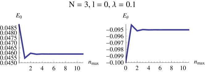
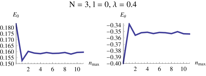
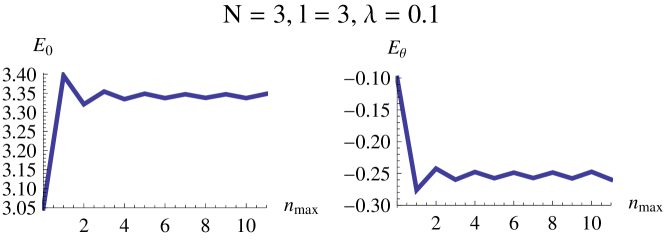
Figure 1: Ground-state (adimensional) energy for the noncommutative anharmonic potential calculated up to order $n_{\mbox{max}}$, in the form $E^{\prime}=E_{0}+E_{\theta}\theta$, for different values of $\ell$ and $\lambda$.

We found that, even using a standard desktop computer, the fully analytical calculation could not be done beyond the $1/N^{3}$ order in reasonable time; however, by choosing some particular numerical values for $\ell$ and $\lambda$, one can quickly calculate the corrections up to $1/N^{12}$ or even more. Some results are shown in graphical form in Fig. (1): the horizontal axis is the order of the $1/N$ expansion used, i.e., for each $n_{\mbox{max}}$ we calculate the adimensional energy $E^{\prime}=E_{0}+\theta E_{\theta}$ up to order $1/N^{n_{\mbox{max}}}$. These graphs suggests that the convergence is quite good, at least for small enough $\lambda$ and for $\ell=0$. For higher $\ell$, the results are not so stable, and the reason is clear from Eq. (37): the first correction for $r_{0}$ is of order $\ell/N$, so Eq. (36) does not provide a good approximation to $r_{0}$ if $\ell$ is not much smaller than $N$.

IV The Noncommutative Coulombian Potential

We now focus on the noncommutative generalization of the Coulombian potential, which is usually given in terms of the noncommutative coordinates $\hat{x}$ as

$$V\left(\hat{x}\right)=-\frac{Ze^{2}}{\sqrt{\hat{x}\hat{x}}}\,.$$ (45)

As described in Sec. II, the customary way to work with this potential is by means of the change of variables in Eq. (3), which yields

$$V\left(x,p\right)=-\frac{Ze^{2}}{\sqrt{r^{2}-\sum_{ij}\theta_{ij}x_{i}p_{j}+\frac{1}{4}\theta_{j\ell}\theta_{jk}p_{\ell}p_{k}}}\,.$$ (46)

A direct treatment of this potential is quite difficult from a technical viewpoint. This is why, in the literature chaichian ; kao ; adorno , it has been studied using standard perturbation theory after an expansion up to the first order in $\theta$ as follows,

$$V=-\frac{Ze^{2}}{r}\left[1+\frac{1}{2r^{2}}\sum_{ij}\theta_{ij}x_{i}p_{j}\right]\,.$$ (47)

We notice that the noncommutative correction to the potential behaves as $1/r^{3}$, so it is more singular at the origin than the one in Eq. (45). We shall also stress that Eq. (47) is not a valid approximation when $r$ is very small. Such issue has not been considered in the literature so far because in standard perturbation theory one is interested in integrals of the general form $\left\langle\psi|V\left(r\right)|\psi\right\rangle$, which are actually regular despite the singularity at the origin. As we shall see, when using the $1/N$ expansion, this singular behavior near the origin will be a major issue we will have to deal with. In this work, we will show how to generalize the potential in Eq. (47) so that it produces a meaningful $1/N$ expansion.

Hereafter, all our expressions are calculated up to the first order in $\theta$. As before, we shall consider the particular case $\theta_{12}=\theta$ with all other components of the matrix $\theta_{ij}$ vanishing, such that $\sum_{ij}\theta_{ij}x_{i}p_{j}=\theta L_{12}$. In this case, $V\left(x,p\right)$ reduces to

$$V\left(r\right)=-\frac{Ze^{2}}{r}\left[1+\theta\frac{L_{12}}{2r^{2}}\right]\,.$$ (48)

We start by taking the potential in Eq. (48) as our starting point. By means of the change of variables

$$\rho=4Z\hat{e}^{2}\,r\quad;\quad\hat{\theta}=\theta\left(4Z\hat{e}^{2}\right)^{2},$$ (49)

the Schr dinger equation becomes

$$\left[-\frac{1}{2}\frac{d^{2}}{d\rho^{2}}+k^{2}V_{\mbox{eff}}\left(\rho\right)+\left(\frac{3}{8}-\frac{1}{2}k\right)\frac{1}{\rho^{2}}\right]\eta\left(\rho\right)=E\eta\left(\rho\right)\,,$$ (50)

with the effective potential

$$V_{\mbox{eff}}\left(\rho\right)=\frac{1}{8\rho^{2}}-\frac{1}{4\rho}-\frac{\hat{\theta}m}{8\rho^{3}}\,.$$ (51)

Here, $\hat{e}^{2}=e^{2}/k^{2}$, $m$ is the eigenvalue of $L_{12}$, and the adimensional energy $E$ is measured in units of $16Z^{2}\hat{e}^{4}$. For simplicity of notation, we shall drop the hat in $\hat{\theta}$ from now on.

The minimum of the effective potential in Eq. (51) is located at

$$\rho_{0}=1-\frac{3\theta m}{2}\,.$$ (52)

The leading approximation to the ground state energy is given by

$$E^{\left(-2\right)}=V_{\mbox{eff}}\left(\rho_{0}\right)=-\frac{(1+\theta\,m)}{8}\,.$$ (53)

To find higher-order corrections, we solve the Riccati equation

$$-\frac{1}{2\rho_{0}^{2}}\left[U^{2}\left(u\right)+U^{\prime}\left(u\right)\right]+k^{2}V_{\mbox{eff}}\left(u\right)+\left(\frac{3}{8}-\frac{1}{2}k\right)\frac{1}{u^{2}}=E\,,$$ (54)

where $u=\rho/\rho_{0}$. Both $U$ and $E$ are expanded in orders of $1/k$ as in Eq. (19). In the leading order, the wavefunction is given by

$$U^{\left(-1\right)}\left(u\right) =-\sqrt{2\rho_{0}^{2}\left(V_{\mbox{eff}}\left(u\right)-V_{\mbox{eff}}\left(1\right)\right)}$$

$$=\frac{1-u}{2u}+\frac{\theta\,m}{4u^{2}}\left(u-1\right)\left(2u+1\right)\,,$$ (55)

whose derivative at $u=1$, using Eq. (21), gives the subleading correction to the energy of the ground state,

$$E^{(-1)}=-\frac{1}{4}\left(1+\frac{9}{2}\theta m\right)\,.$$ (56)

Inserting back this value of $E^{(-1)}$ in Eq. (21), one obtains the subleading contribution to the wavefunction,

$$U^{\left(0\right)}\left(u\right)=-\frac{u+1}{2u}-\frac{5u^{2}+6u+3}{4u^{2}}\theta m\,.$$ (57)

For the noncommutative Coulombian potential, this procedure can be repeated to higher orders in $1/k$. A simple computer program was used to calculate both $E^{\left(n\right)}$ and $U^{\left(n\right)}$ up to $n_{\mbox{max}}\sim 50$ in a few seconds. Up to order $1/k^{10}$, the energy of the ground state was calculated as

$$E= -\frac{\kappa}{4}-\frac{3}{8}-\frac{1}{2\kappa}-\frac{5}{8\kappa^{2}}-\frac{3}{4\kappa^{3}}-\frac{7}{8\kappa^{4}}-\frac{1}{\kappa^{5}}$$

$$-\frac{9}{8\kappa^{6}}-\frac{5}{4\kappa^{7}}-\frac{11}{8\kappa^{8}}-\frac{3}{2\kappa^{9}}-\frac{13}{8\kappa^{10}}$$

$$+\theta\left(-\frac{9\kappa}{8}-\frac{49}{8}-\frac{211}{8\kappa}-\frac{199}{2\kappa^{2}}-\frac{1385}{4\kappa^{3}}-\frac{4579}{4\kappa^{4}}-\frac{14645}{4\kappa^{5}}\right.$$

$$\left.-\frac{91667}{8\kappa^{6}}-\frac{282815}{8\kappa^{7}}-\frac{864359}{8\kappa^{8}}-\frac{2625269}{8\kappa^{9}}-\frac{3970323}{4\kappa^{10}}\right)\,.$$ (58)

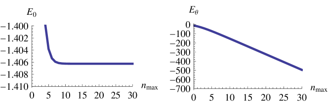
Figure 2: Ground-state energy of the noncommutative Coulombian potential calculated up to the order $1/k^{n_{\mbox{max}}}$.

From this result, we see a quite different behavior for the $\theta$-independent terms and for the $\theta$-dependent ones. This result is graphically represented in Fig. 2; the $\theta$-independent contribution to the energy converges quickly and this convergence is very stable for higher orders of $1/k$, while the $\theta$-dependent ones badly diverges.

Divergences of the $1/N$ expansion are not surprising, since the expansion is usually stable up to some order but it diverges at higher orders (see for example bohr ). However, in our case, there is no convergence at all, so the $1/N$ expansion does not provide a useful calculational scheme. However, it is interesting to notice that this problem is restricted to the $\theta$-dependent part of the energy, so its origin is in the noncommutative part of the potential. The main particularity of this term is the stronger singularity at the origin, and we will now show that modifying the potential in Eq. (48) to soften this singularity will indeed avoid the divergence of the $1/N$ expansion.

We propose a modified version of the noncommutative Coulombian potential as follows,

$$V\left(r\right)=-\frac{Z\hat{e}^{2}}{r}\left[1+\frac{m}{2r^{2}}\left(1-e^{-\alpha r^{\beta}}\right)\frac{\theta}{k}\right]\,.$$ (59)

With this modification, the noncommutative part of the potential behaves as $1/r^{3-\beta}$ near the origin, so it is actually less divergent than the usual Coulombian potential if $\beta>2$. The factor $\alpha$ has dimension $\left[\mbox{length}\right]^{-\beta}$, so it defines the characteristic length scale of the modification we are introducing. In proposing this potential, we have also redefined the noncommutativity parameter $\theta$ as $\theta\rightarrow\theta/k$: this is needed because, due to the exponential function in Eq. (59), the equation defining $r_{0}$ would be transcendental and no analytic solution could be found foot1 . With the rescaling $\theta\rightarrow\theta/k$, the effective potential does not include any $\theta$-dependence,

$$V_{\mbox{eff}}\left(r\right)=\frac{1}{8r^{2}}-\frac{Z\hat{e}^{2}}{r}\,,$$ (60)

and all the modification due to the noncommutativity enters through subleadings corrections obtained from the Riccati equation,

$$-\frac{1}{2r_{0}^{2}}\left[U^{2}\left(u\right)+U^{\prime}\left(u\right)\right]+k^{2}V_{\mbox{eff}}(u)-\frac{k}{2}\left[\frac{1}{r_{0}^{2}u^{2}}+\frac{Z\hat{e}^{2}}{r_{0}^{3}u^{3}}\theta m\left(1-e^{-\alpha r^{\beta}}\right)\right]+\frac{3}{8}\frac{1}{r_{0}^{2}u^{2}}=E.$$ (61)

We remark that such rescalings are usual in $1/k$ expansion, as discussed in kalara .

By redefining coordinates as

$$\rho=4Z\hat{e}^{2}\,r\hskip 8.5359pt;\hskip 8.5359pt\tilde{\theta}=\theta\left(4Z\hat{e}^{2}\right)^{2}\hskip 8.5359pt;\hskip 8.5359pt\tilde{\alpha}=\frac{\alpha}{(4Z\hat{e}^{2})^{\beta}}\hskip 8.5359pt;\hskip 8.5359pt\tilde{E}=E/\left(4Z\hat{e}^{2}\right)^{2}$$ (62)

we rewrite Eq. (61) as (dropping the tildes)

$$-\frac{1}{2}\left[U^{2}\left(\rho\right)+U^{\prime}\left(\rho\right)\right]+k^{2}V_{\mbox{eff}}\left(\rho\right)-k\left[\frac{1}{2\rho^{2}}+\frac{\theta m}{8\rho^{3}}\left(1-e^{-\alpha\rho^{\beta}}\right)\right]+\frac{3}{8\rho^{2}}=E\,,$$ (63)

where the effective potential is given by Eq. (60). The minimum of $V_{\mbox{eff}}\left(\rho\right)$ is located at $\rho_{0}=1$, the leading order energy reads $E^{\left(-2\right)}=-1/4$ and

$$U^{(-1)}=\frac{1-\rho}{2\rho}\,,$$ (64)

which is the same as the commutative case. We follow the procedure outlined in Sec. II to calculate higher order corrections to $E$ and $U$, the only modification is in Eq. (21) for the subleading order, which is modified to

$$-\frac{1}{2}\left[2U^{(-1)}U^{(0)}+U^{(-1)\prime}\right]-\frac{1}{2\rho^{2}}-\frac{\theta m}{8\rho^{3}}\left(1-e^{-\alpha\rho^{\beta}}\right)=E^{(-1)}\,,$$ (65)

now including the noncommutative correction, which will therefore appear starting in the subleading order.

We have calculated analytically the energy up to the order $1/k^{8}$ using a Mathematica program, and we plotted $E=E_{0}+\theta E_{\theta}$ for several orders of the $1/k$ expansion, looking for values for $\alpha$ and $\beta$ which would provide a reasonably convergence and stability of the $1/k$ expansion. Some results are depicted in Fig. 3. We found that for $\alpha$ of order unity and $\beta=2$ we obtained the best convergence results. In this situation, we obtained

$$E= -0.25\kappa-0.375-\frac{0.5}{\kappa}-\frac{0.625}{\kappa^{2}}-\frac{0.75}{\kappa^{3}}-\frac{0.875}{\kappa^{4}}-\frac{1.0}{\kappa^{5}}-\frac{1.125}{\kappa^{6}}-\frac{1.25}{\kappa^{7}}-\frac{1.375}{\kappa^{8}}$$

$$\theta\left(-0.0790151\kappa-0.297271-\frac{0.338563}{\kappa}-\frac{0.592782}{\kappa^{2}}-\frac{0.393406}{\kappa^{3}}\right.$$

$$\left.-\frac{1.40262}{\kappa^{4}}+\frac{0.674301}{\kappa^{5}}-\frac{2.54331}{\kappa^{6}}-\frac{15.0062}{\kappa^{7}}+\frac{124.537}{\kappa^{8}}\right)\,.$$ (66)

For smaller $\alpha$, the convergence is even better, but this would imply in a larger length scale of the modification, which may be not natural. In Fig. 4 we present our results for fixed $\beta=2$ and different values of $\alpha$, showing that if $\alpha$ is taken to be greater than one, the convergence of the $1/N$ expansion is not adequate.

V Conclusions

In this work, we studied the noncommutative quantum mechanics using the $1/N$ expansion for the anharmonic and Coulombian potential. We showed that, for a particular choice of the noncommutativity matrix $\theta_{ij}$, we could apply the $1/N$ expansion for a noncommutative potential depending only on a noncommutativity scalar parameter $\theta$. With this simplification, we studied the anharmonic oscillator, calculating the ground state energy up to the order $1/N^{12}$. For this potential, the expansion presented good convergence properties.

For the Coulombian potential, however, the usual procedure of expanding in powers of the noncommutative matrix is invalid leading to a divergent $1/N$ expansion. In fact, the noncommutative modication to the potential,

$$\frac{Z\hat{e}^{2}}{2r^{3}}\theta m\,,$$ (67)

is highly singular near $r=0$. We therefore proposed a modified version of the noncommutative Coulombian potential, where Eq. (67) is replaced by

$$\left(1-e^{-\alpha r^{\beta}}\right)\frac{Z\hat{e}^{2}}{2r^{3}}\theta m\,.$$ (68)

The included term, $\frac{Z\hat{e}^{2}}{2r^{3}}e^{-\alpha r^{\beta}}\theta m$, vanish exponentially for large $r$, so this modification is intended to modify the potential in the $r\sim 0$ region, softening the singularity at the origin. We calculated the ground-state energy of such a modified potential up to the order $1/N^{7}$, finding a good convergence for certain values of $\alpha$ and $\beta$. The best choice for $\beta$ is $\beta=2$, and for $\alpha$, the range $0<\alpha<1$ provided a well-behaved expansion.

We concluded that the $1/N$ expansion can indeed be applied in noncommutative quantum mechanical systems, but it seems more sensitive to the singularities of the potential than the usual perturbative expansion.

Acknowledgments. This work was partially supported by the Brazilian agencies Conselho Nacional de Desenvolvimento Científico e Tecnológico (CNPq) and Fundação de Amparo à Pesquisa do Estado de São Paulo (FAPESP).

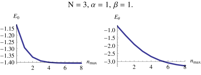
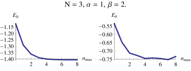
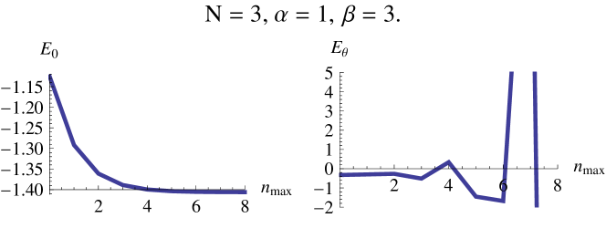
Figure 3: Ground-state energy of the modified noncommutative Coulombian potential calculated up to the order $1/k^{n_{\mbox{max}}}$, for different values of $\alpha$ and $\beta$.

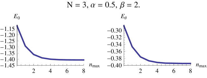
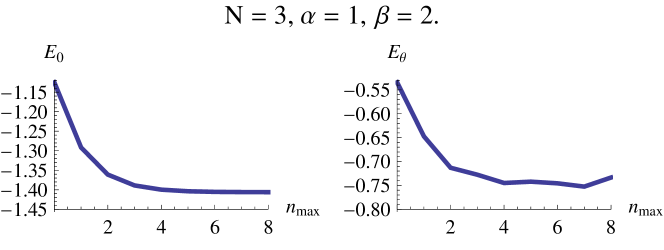
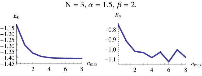
Figure 4: Same as in Fig. 3, for fixed $\beta=2$ and different values of $\alpha$.

References

• (1) ’t Hooft, Nucl. Phys. B 72, 461 (1974).
• (2) A. V. Manohar, β€œLarge N QCD”, published in β€œLes Houches 1997, Probing the standard model of particle interactions, Pt. 2”, F. David & R. Gupta eds., Amsterdam, North-Holland, 1999, hep-ph/9802419.
• (3) S. Coleman, β€œ1/N” in β€œAspects of Symmetry”, Cambridge University Press, 1985.
• (4) Ch. Moseley and K. Ziegler, Laser Physics, 15, 469 (2005).
• (5) H. Babujian, A. Foerster and M. Karowski, Nucl. Phys. B 825, 396 (2010).
• (6) J. C. Brunelli and M. Gomes, Phys. Rev. D 46, 2617 (1992).
• (7) E. A. Asano, H. O. Girotti, M. Gomes, A. Yu. Petrov, A. G. Rodrigues and A. J. da Silva, Phys. Rev. D 69, 105012 (2004).
• (8) E. A. Asano, M. Gomes, A. G. Rodrigues, and A. J. da Silva, Phys. Rev. D 69, 065012 (2004).
• (9) E. T. Akhmedov, P. DeBoer and G. W. Semenoff, J. High En. Phys. 06, 009 (2001); H. Girotti, M. Gomes, V. O. Rivelles, A. J. da Silva, Int. J. Mod. Phys. A 17, 1503 (2002).
• (10) J. Maldacena, Adv. Theor. Math. Phys. 2, 231 (1998).
• (11) N. Seiberg, E. Witten, JHEP 09, 032 (1999).
• (12) S. Doplicher, K. Fredenhagen, J. E. Roberts, Commun. Math. Phys. 172, 187 (1995).
• (13) J. Gamboa, M. Loewe and J. C. Rojas, Phys. Rev. D 64, 067901 (2001).
• (14) M. Chaichian, M. M. Sheikh-Jabbari and A. Tureanu, Phys. Rev. Lett. 86, 2716 (2001); Eur. Phys. J. C 36, 251 (2004).
• (15) M. Lubo, Phys. Rev. D 65, 066003 (2002).
• (16) H. R. Christiansen and F. A. Schaposnik, Phys. Rev. D 65, 086005 (2002).
• (17) B. Muthukumar, P. Mitra, Phys. Rev. D 66, 027701 (2002).
• (18) H. O. Girotti, β€œNoncommutative Quantum Field Theories”, hep-th/0301237 (2003).
• (19) A. F. Ferrari, M. Gomes, C. A. Stechhahn, Phys. Rev. D 76, 085008 (2007).
• (20) M. Gomes and V. G. Kupriyanov, Phys. Rev. D 79, 125011 (2009); M. Gomes, V. G. Kupriyanov and A. J. da Silva, J. Phys. A 43, 285301 (2010); M. Gomes, V. G. Kupriyanov and A. J. da Silva, Phys. Rev. D 81, 085024 (2010).
• (21) L. D. Mlodinow, M. P. Shatz, J. Math. Phys. 25, 943 (1984).
• (22) J. D. Louck, J. Mol. Spectr. 4, 298 (1960).
• (23) S. Kalara, β€œ1/N Expansion In Quantum Mechanics: Formalism And Applications,” Rochester Preprint COO-3065-323, 1982.
• (24) A. V. Koudinov, M. A. Smondyrev, Chz. J. Phys. 32, 556 (1982); Th. and Math. Phys. 56, 871 (1983).
• (25) P.-M. Ho and H.-C. Kao, Phys. Rev. Lett. 88, 151602 (2002).
• (26) T. C. Adorno, M. C. Baldiotti, M. Chaichian, D. M. Gitman and A. Tureanu, Phys. Lett. B 682, 235 (2009) .
• (27) N. E. J. Bjerrum-Bohr, J. Math. Phys. 41, 2515 (2000).
• (28) Such a transcendental equation could only be solved by numerical methods, but the method we are using is not well suited for numerical calculations: as it becomes clear from Eqs. (21) to (23), at a given order $1/k^{n}$, the wavefunction correction $U^{\left(n+1\right)}$ is a function possesing a potential $0/0$ singularity at $u=1$, so it is difficult to evaluate numerically such functions at $u=1$. This is a major stumbling block since the energies at each order are calculated exactly by evaluating the r.h.s of Eqs. (21) to (23) at $u=1$.
Refer to caption
Refer to caption
Refer to caption