Compressed Sensing with Coherent and Redundant Dictionaries

Abstract

This article presents novel results concerning the recovery of signals from undersampled data in the common situation where such signals are not sparse in an orthonormal basis or incoherent dictionary, but in a truly redundant dictionary. This work thus bridges a gap in the literature and shows not only that compressed sensing is viable in this context, but also that accurate recovery is possible via an $\ell_{1}$-analysis optimization problem. We introduce a condition on the measurement/sensing matrix, which is a natural generalization of the now well-known restricted isometry property, and which guarantees accurate recovery of signals that are nearly sparse in (possibly) highly overcomplete and coherent dictionaries. This condition imposes no incoherence restriction on the dictionary and our results may be the first of this kind. We discuss practical examples and the implications of our results on those applications, and complement our study by demonstrating the potential of $\ell_{1}$-analysis for such problems.

1 Introduction

Compressed sensing is a new data acquisition theory based on the discovery that one can exploit sparsity or compressibility when acquiring signals of general interest, and that one can design nonadaptive sampling techniques that condense the information in a compressible signal into a small amount of data [13, 16, 18]. In a nutshell, reliable, nonadaptive data acquisition, with far fewer measurements than traditionally assumed, is possible. By now, applications of compressed sensing are abundant and range from imaging and error correction to radar and remote sensing, see [2, 1] and references therein.

In a nutshell, compressed sensing proposes acquiring a signal $x\in\mathbb{R}^{n}$ by collecting $m$ linear measurements of the form $y_{k}=\langle a_{k},x\rangle+z_{k}$, $1\leq k\leq m$, or in matrix notation,

$$y=Ax+z;$$ (1.1)

$A$ is an $m\times n$ sensing matrix with $m$ typically smaller than $n$ by one or several orders of magnitude (indicating some significant undersampling) and $z$ is an error term modeling measurement errors. Sensing is nonadaptive in that $A$ does not depend on $x$. Then the theory asserts that if the unknown signal $x$ is reasonably sparse, or approximately sparse, it is possible to recover $x$, under suitable conditions on the matrix $A$, by convex programming: we simply find the solution to

$$\min_{\tilde{x}\in\mathbb{R}^{n}}\|\tilde{x}\|_{1}\quad\text{subject to}\quad\|A\tilde{x}-y\|_{2}\leq\varepsilon, L_{1}$$ ()

where $\|\cdot\|_{2}$ denotes the standard Euclidean norm, $\|x\|_{1}=\sum|x_{i}|$ is the $\ell_{1}$-norm and $\varepsilon^{2}$ is a likely upper bound on the noise power $\|z\|_{2}^{2}$. (There are other algorithmic approaches to compressed sensing based on greedy algorithms such as Orthogonal Matching Pursuit [31, 42], Iterative Thresholding [7, 23], Compressive Sampling Matching Pursuit [34], and many others.)

Quantitatively, a concrete example of a typical result in compressed sensing compares the quality of the reconstruction from the data $y$ and the model (1.1) with that available if one had an oracle giving us perfect knowledge about the most significant entries of the unknown signal $x$. Define – here and throughout – by $x_{s}$ the vector consisting of the $s$ largest coefficients of $x\in\mathbb{R}^{n}$ in magnitude:

$$x_{s}=\operatorname*{argmin}_{\|\tilde{x}\|_{0}\leq s}\|x-\tilde{x}\|_{2},$$ (1.2)

where $\|x\|_{0}=|\{i:x_{i}\neq 0\}|$. In words, $x_{s}$ is the best $s$-sparse approximation to the vector $x$, where we shall say that a vector is $s$-sparse if it has at most $s$ nonzero entries. Put differently, $x-x_{s}$ is the tail of the signal, consisting of the smallest $n-s$ entries of $x$. In particular, if $x$ is $s$-sparse, $x-x_{s}=0$. Then with this in mind, one of the authors [9] improved on the work of Candès, Romberg and Tao [14] and established that $(L_{1})$ recovers a signal $\hat{x}$ obeying

$$\|\hat{x}-x\|_{2}\leq C_{0}\frac{\|x-x_{s}\|_{1}}{\sqrt{s}}+C_{1}\varepsilon,$$ (1.3)

provided that the $2s$-restricted isometry constant of $A$ obeys $\delta_{2s}<\sqrt{2}-1$. The constants in this result have been further improved, and it is now known to hold when $\delta_{2s}<0.4652$ [24], see also [25]. In short, the recovery error from $(L_{1})$ is proportional to the measurement error and the tail of the signal. This means that for compressible signals, those whose coefficients obey a power law decay, the approximation error is very small, and for exactly sparse signals it completely vanishes.

The definition of restricted isometries first appeared in [15] where it was shown to yield the error bound (1.3) in the noiseless setting, i. e. when $\varepsilon=0$ and $z=0$.

Definition 1.1

For an $m\times n$ measurement matrix $A$, the $s$-restricted isometry constant $\delta_{s}$ of $A$ is the smallest quantity such that

$$(1-\delta_{s})\|x\|_{2}^{2}\leq\|Ax\|_{2}^{2}\leq(1+\delta_{s})\|x\|_{2}^{2}$$

holds for all $s$-sparse signals $x$.

With this, the condition underlying (1.3) is fairly natural since it is interpreted as preventing sparse signals from being in the nullspace of the sensing matrix $A$. Further, a matrix having a small restricted isometry constant essentially means that every subset of $s$ or fewer columns is approximately an orthonormal system. It is now well known that many types of random measurement matrices have small restricted isometry constants [16, 32, 37, 6]. For example, matrices with Gaussian or Bernoulli entries have small restricted isometry constants with very high probability whenever the number of measurements $m$ is on the order of $s\log(n/s)$. The fast multiply matrix consisting of randomly chosen rows of the discrete Fourier matrix also has small restricted isometry constants with very high probability with $m$ on the order of $s(\log n)^{4}$.

1.1 Motivation

The techniques above hold for signals which are sparse in the standard coordinate basis or sparse with respect to some other orthonormal basis. However, there are numerous practical examples in which a signal of interest is not sparse in an orthonormal basis. More often than not, sparsity is expressed not in terms of an orthonormal basis but in terms of an overcomplete dictionary. This means that our signal $f\in\mathbb{R}^{n}$ is now expressed as $f=Dx$ where $D\in\mathbb{R}^{n\times d}$ is some overcomplete dictionary in which there are possibly many more columns than rows. The use of overcomplete dictionaries is now widespread in signal processing and data analysis, and we give two reasons why this is so. The first is that there may not be any sparsifying orthonormal basis, as when the signal is expressed using curvelets [11, 10] or time-frequency atoms as in the Gabor representation [22]. In these cases and others, no good orthobases are known to exist and researchers work with tight frames. The second reason is that the research community has come to appreciate and rely on the flexibility and convenience offered by overcomplete representations. In linear inverse problems such as deconvolution and tomography for example – and even in straight signal-denoising problems where $A$ is the identity matrix – people have found overcomplete representations to be extremely helpful in reducing artifacts and mean squared error (MSE) [39, 40]. It is only natural to expect overcomplete representations to be equally helpful in compressed sensing problems which, after all, are special inverse problems.

Although there are countless applications for which the signal of interest is represented by some overcomplete dictionary, the compressed sensing literature is lacking on the subject. Consider the simple case in which the sensing matrix $A$ has Gaussian (standard normal) entries. Then the matrix $AD$ relating the observed data with the assumed (nearly) sparse coefficient sequence $x$ has independent rows but each row is sampled from $\mathcal{N}(0,\Sigma)$, where $\Sigma=D^{*}D$. If $D$ is an orthonormal basis, then these entries are just independent standard normal variables, but if $D$ is not unitary then the entries are correlated, and $AD$ may no longer satisfy the requirements imposed by traditional compressed sensing assumptions. In [35] recovery results are obtained when the sensing matrix $A$ is of the form $\Phi D^{*}$ where $\Phi$ satisfies the restricted isometry property. In this case the sampling matrix must depend on the dictionary $D$ in which the signal is sparse. We look for a universal result which allows the sensing matrix to be independent from the signal and its representation. To be sure, we are not aware of any such results in the literature guaranteeing good recovery properties when the columns may be highly – and even perfectly – correlated.

Before continuing, it might be best to fix ideas to give some examples of applications in which redundant dictionaries are of crucial importance.

Oversampled DFT

The Discrete Fourier Transform (DFT) matrix is an $n\times n$ orthogonal matrix whose $k$th column is given by

$$d_{k}(t)=\frac{1}{\sqrt{n}}e^{-2\pi ikt/n},$$

with the convention that $0\leq t,k\leq n-1$. Signals which are sparse with respect to the DFT are only those which are superpositions of sinusoids with frequencies appearing in the lattice of those in the DFT. In practice, we of course rarely encounter such signals. To account for this, one can consider the oversampled DFT in which the sampled frequencies are taken over even smaller equally spaced intervals, or at small intervals of varying lengths. This leads to an overcomplete frame whose columns may be highly correlated.

Gabor frames

Recall that for a fixed function $g$ and positive time-frequency shift parameters $a$ and $b$, the $k$th column (where $k$ is the double index $k=(k_{1},k_{2})$) of the Gabor frame is given by

$$G_{k}(t)=g(t-k_{2}a)e^{2\pi ik_{1}bt}.$$ (1.4)

Radar and sonar along with other imaging systems appear in many engineering applications, and the goal is to recover pulse trains given by

$$f(t)=\sum_{j=1}^{k}\alpha_{j}w\Big{(}\frac{t-t_{j}}{\sigma_{j}}\Big{)}\mathrm{e}^{i\omega_{j}t}.$$

Due to the time-frequency structure of these applications, Gabor frames are widely used [30]. If one wishes to recover pulse trains from compressive samples by using a Gabor dictionary, standard results do not apply.

Curvelet frames

Curvelets provide a multiscale decomposition of images, and have geometric features that set them apart from wavelets and the likes. Conceptually, the curvelet transform is a multiscale pyramid with many directions and positions at each length scale, and needle-shaped elements at fine scales [11]. The transform gets its name from the fact that it approximates well the curved singularities in an image. This transform has many properties of an orthonormal basis, but is overcomplete. Written in matrix form $D$, it is a tight frame obeying the Parseval relations

$$f=\sum_{k}\langle f,d_{k}\rangle d_{k}\quad\text{and}\quad\|f\|_{2}^{2}=\sum_{k}|\langle f,d_{k}\rangle|^{2},$$

where we let $\{d_{k}\}$ denote the columns of $D$. Although columns of $D$ far apart from one another are very uncorrelated, columns close to one another have high correlation. Thus none of the results in compressed sensing apply for signals represented in the curvelet domain.

Wavelet Frames

The undecimated wavelet transform (UWT) is a wavelet transform achieving translation invariance, a property that is missing in the discrete wavelet transform (DWT) [20]. The UWT lacks the downsamplers and upsamplers in the DWT but upsamples the filter coefficients by a factor of $2^{m}$ at the $(m-1)$st level – hence it is overcomplete. Also, the Unitary Extension Principle of Ron and Shen [36] facilitates tight wavelet frame constructions for $L^{2}(\mathbb{R}^{d})$ which may have many more wavelets than in the orthonormal case. This redundancy has been found to be helpful in image processing (see e.g. [39]), and so one wishes for a recovery result allowing for significant redundancy and/or correlation.

Concatenations

In many applications a signal may not be sparse in a single orthonormal basis, but instead is sparse over several orthonormal bases. For example, a linear combination of spikes and sines will be sparse when using a concatenation of the coordinate and Fourier bases. One also benefits by exploiting geometry and pointwise singularities in images by using combinations of tight frame coefficients such as curvelets, wavelets, and brushlets. However, due to the correlation between the columns of these concatenated bases, current compressed sensing technology does not apply.

These and other applications strongly motivate the need for results applicable when the dictionary is redundant and has correlations. This state of affair, however, exposes a large gap in the literature since current compressed sensing theory only applies when the dictionary is an orthonormal basis, or when the dictionary is extremely uncorrelated (see e.g. [26, 38, 5]).

1.2 Do we really need incoherence?

Current assumptions in the field of compressed sensing and sparse signal recovery impose that the measurement matrix have uncorrelated columns. To be formal, one defines the coherence of a matrix $M$ as

$$\mu(M)=\max_{j<k}\frac{|\langle M_{j},M_{k}\rangle|}{\|M_{j}\|_{2}\|M_{k}\|_{2}},$$

where $M_{j}$ and $M_{k}$ denote columns of $M$. We say that a dictionary is incoherent if $\mu$ is small. Standard results then require that the measurement matrix satisfy a strict incoherence property [41, 12], as even the RIP imposes this. If the dictionary $D$ is highly coherent, then the matrix $AD$ will also be coherent in general.

Coherence is in some sense a natural property in the compressed sensing framework, for if two columns are closely correlated, it will be impossible in general to distinguish whether the energy in the signal comes from one or the other. For example, imagine that we are not undersampling and that $A$ is the identity so that we observe $y=Dx$. Suppose the first two columns are identical, $d_{1}=d_{2}$. Then the measurement $d_{1}$ can be explained by the input vectors $(1,0,\ldots,0)$ or $(0,1,0,\ldots,0)$ or any convex combination. Thus there is no hope of reconstructing a unique sparse signal $x$ from measurements $y=ADx$. However, we are not interested in recovering the coefficient vector $x$, but rather the actual signal $Dx$. The large correlation between columns in $D$ now does not impose a problem because although it makes it impossible to tell apart coefficient vectors, this is not the goal. This simple example suggests that perhaps coherence is not necessary. If $D$ is coherent, then we clearly cannot recover $x$ as in our example, but we may certainly be able to recover the signal $f=Dx$ from measurements $y=Af$ as we shall see next.

Figure 1: The compressed sensing process and its domains. This distinguishes the domains in which the measurements, signals, and coefficients reside

1.3 Gaussian sensing matrices

To introduce our results, it might be best for pedagogical purposes to discuss a concrete situation first, and we here assume that the sensing matrix has iid Gaussian entries. In practice, signals are never exactly sparse, and dictionaries are typically designed to make $D^{*}f$ for some classes of $f$ as sparse as possible. Therefore, in this paper, we propose a reconstruction from $y=Af+z$ by the method of $\ell_{1}$-analysis:

$$\hat{f}=\operatorname*{argmin}_{\tilde{f}\in\mathbb{R}^{n}}\|D^{*}\tilde{f}\|_{1}\quad\text{subject to}\quad\|A\tilde{f}-y\|_{2}\leq\varepsilon, P_{1}$$ ()

where again $\varepsilon$ is a likely upper bound on the noise level $\|z\|_{2}$. Empirical studies have shown very promising results for the $\ell_{1}$-analysis problem. Its geometry has been studied [21] as well as its applications to image restoration [8]. However, there are no results in the literature about its performance.

Our main result is that the solution to $(P_{1})$ is very accurate provided that $D^{*}f$ has rapidly decreasing coefficients. Our result for the Gaussian case is below while the general theorem appears in Section 1.5.

Theorem 1.2

Let $D$ be an arbitrary $n\times d$ tight frame and let $A$ be a $m\times n$ Gaussian matrix with $m$ on the order of $s\log(d/s)$. Then the solution $\hat{f}$ to $(P_{1})$ obeys

$$\|\hat{f}-f\|_{2}\leq C_{0}\varepsilon+C_{1}\frac{\|D^{*}f-(D^{*}f)_{s}\|_{1}}{\sqrt{s}},$$

for some numerical constants $C_{0}$ and $C_{1}$, and where $(D^{*}f)_{s}$ is the vector consisting of the largest $s$ entries of $D^{*}f$ in magnitude as in (1.2).

We have assumed that $D$ is a tight frame although this is simply to make the analysis easier and is of course not necessary. Having said this, our results proves not only that compressed sensing is viable with highly coherent dictionaries, but also that the $\ell_{1}$-analysis problem provably works in this setting. We are not aware of any other result of this kind. To be sure, other methods for redundant dictionaries such as [38, 5, 41] force incoherence on the dictionary $D$ so that the matrix $AD$ conforms to standard compressed sensing results. The method in [35] requires that the sensing matrix depend on the dictionary. These are drastically different from the setting here, where we impose no such properties on the dictionary. We point out that our result holds even when the coherence of the dictionary $D$ is maximal, meaning two columns are completely correlated. Finally, we also note that the dependence on the noise level is optimal and that the tail bound in the error is analogous to previous bounds in the non-redundant case such as (1.3).

1.4 Implications

As we mentioned, the dependence on the noise in the error given by Theorem 1.2 is optimal, and so we need only discuss how the second term affects the estimation error. This term will of course be negligible when the norm of the tail, $D^{*}f-(D^{*}f)_{s}$, is small. Hence, the result says that for any dictionary, signals $f$ such that $D^{*}f$ decays rapidly can be approximately reconstructed using $\ell_{1}$-analysis from just a few random measurements. This is exactly the case for many dictionaries used in practice and many classes of signals as discussed earlier. As a side remark, one can also guarantee rapid decay of $D^{*}f$ (we assume the signal expansion $f=Dx$) when $D^{*}D$ is well behaved and the coefficient vector $x$ is nearly sparse. To see why this is true, suppose $D$ is a tight frame so that $D^{*}f=D^{*}Dx$. A norm commonly used to quantify sparsity is the quasi $p$-norm with $p\leq 1$ defined via $\|x\|_{p}^{p}=\sum_{i}|x_{i}|^{p}$ (sparser signals with unit $2$-norm have smaller $p$-norms). Now a simple calculation shows that

$$\|D^{*}f\|_{p}\leq\Bigl{[}\max_{j}\sum_{i}|(D^{*}D)_{ij}|^{p}\Bigr{]}^{1/p}\,\|x\|_{p}.$$

In words, if the columns of the Gram matrix are reasonably sparse and if $f$ happens to have a sparse expansion, then the frame coefficient sequence $D^{*}f$ is also sparse. All the transforms discussed above, namely, the Gabor, curvelet, wavelet frame, oversampled Fourier transform all have nearly diagonal Gram matrices – and thus, sparse columns.

We now turn to the implications of our result to the applications we have already mentioned, and instantiate the theorem in the noiseless case due to the optimality of the noise level in the error.

Multitone signals

To recover multitone signals, we use an oversampled DFT, which is not orthonormal and may have very large coherence. However, since each “off-grid” tone has a rapidly decaying expansion, $D^{*}f$ will have rapidly decaying coefficients. Thus our result implies that the recovery error is negligible when the number of measurements is about the number of tones times a log factor.

Radar

For radar and sonar applications using Gabor dictionaries, our result similarly implies a negligible error. Indeed, with notation as in (1.4), one sees that the sequence $\{\langle w(t)\mathrm{e}^{i\omega t},G_{k}(t)\rangle\}_{k}$ decays quickly (each pulse has a rapidly decaying expansion). Therefore, our result implies a negligible error when the number of measurements is roughly the number of pulses in the pulse train, up to a log factor.

Images

Roughly speaking, the curvelet coefficient sequence of an arbitrary image, which is discontinuous along piecewise-$C^{2}$ edges but is otherwise smooth, decays like $k^{-3/2}$ – up to a log factor – when arranged in a decreasing order of magnitude. Hence, our theorem asserts that one can get an $\ell_{2}$ error of about $s^{-1}$ from about $s\log n$ random samples of $f$. This is interesting since this is the approximation error one would get by bandlimiting the image to a spatial frequency about equal to $s$ or, equivalently, by observing the first $s^{2}$ Fourier coefficients of $f$. So even though we do not know where the edges are, this says that one can sense an image nonadaptively $m$ times, and get a recovery error which is as good as that one would traditionally get by taking a much larger number – about $m^{2}$ – of samples. This is a considerable gain. Of course, similar implications hold when the undecimated wavelet transform of those images under study decay rapidly.

Concatenations

When working with signals which are sparse over several orthonormal bases, it is natural to use a dictionary $D$ consisting of a concatenation of these bases. For example, consider the dictionary $D$ which is the concatenation of the identity and the Fourier basis (ignoring normalizations for now). Then $D^{*}D$ is made up of four blocks, two of which are the identity and two of which are the DFT, and does not have sparse columns. Then even when $f$ is sparse in $D$, the coefficients of $D^{*}f$ may be spread. If this is the case, then the theorem does not provide a good error bound. This should not be a surprise however, for if $D^{*}f$ is not close to a sparse signal, then we do not expect $f$ to be the minimizer of the $\ell_{1}$-norm in $(P_{1})$. In this case, $\ell_{1}$-analysis is simply not the right method to use.

To summarize, we see that in the majority of the applications, our theorem yields good recovery results. As seen in the last example, the $\ell_{1}$-analysis method only makes sense when $D^{*}f$ has quickly decaying coefficients, which may not be the case for concatenations of orthonormal bases. However, this is not always the case, as we see in the following.

An easy example. As above, let $D$ be the $n\times 2n$ dictionary consisting of a concatenation of the identity and the DFT, normalized to ensure $D$ is a tight frame (below, $F$ is the DFT normalized to be an isometry):

$$D=\frac{1}{\sqrt{2}}[I\quad F].$$

We wish to create a sparse signal that uses linearly dependent columns for which there is no local isometry. Assume that $n$ is a perfect square and consider the Dirac comb

$$f(t)=\sum_{j=1}^{\sqrt{n}}\delta(t-j\sqrt{n}),$$

which is a superposition of spikes spread $\sqrt{n}$ apart. Thus our signal is a sparse linear combination of spikes and sines, something that by the last example alone we would not expect to be able to recover. However, $D^{*}f=[f\quad f]/\sqrt{2}$ is exactly sparse implying that $\|D^{*}f-(D^{*}f)_{s}\|_{1}=0$ when $s>2\sqrt{n}$. Thus our result shows that $\ell_{1}$-analysis can exactly recover the Dirac comb consisting of spikes and sines from just a few general linear functionals.

1.5 Axiomization

We now turn to the generalization of the above result, and give broader conditions about the sensing matrix under which the recovery algorithm performs well. We will impose a natural property on the measurement matrix, analogous to the restricted isometry property.

Definition 1.3 (D-RIP)

Let $\Sigma_{s}$ be the union of all subspaces spanned by all subsets of $s$ columns of $D$. We say that the measurement matrix $A$ obeys the restricted isometry property adapted to $D$ (abbreviated D-RIP) with constant $\delta_{s}$ if

$$(1-\delta_{s})\|v\|_{2}^{2}\leq\|Av\|_{2}^{2}\leq(1+\delta_{s})\|v\|_{2}^{2}$$

holds for all $v\in\Sigma_{s}$.

We point out that $\Sigma_{s}$ is just the image under $D$ of all $s$-sparse vectors. Thus the D-RIP is a natural extension to the standard RIP. We will see easily that Gaussian matrices and other random compressed sensing matrices satisfy the D-RIP. In fact any $m\times n$ matrix $A$ obeying for fixed $v\in\mathbb{R}^{n}$,

$$\mathbb{P}\big{(}(1-\delta)\|v\|_{2}^{2}\leq\|Av\|_{2}^{2}\leq(1+\delta)\|v\|_{2}^{2}\big{)}\leq C\mathrm{e}^{-\gamma m}$$ (1.5)

($\gamma$ is an arbitrary positive numerical constant) will satisfy the D-RIP with overwhelming probability, provided that $m\gtrsim s\log(d/s)$. This can be seen by a standard covering argument (see e.g. the proof of Lemma 2.1 in [38]). Many types of random matrices satisfy (1.5). It is now well known that matrices with Gaussian, subgaussian, or Bernoulli entries satisfy (1.5) with number of measurements $m$ on the order of $s\log(d/s)$ (see e.g. [6]). It has also been shown [32] that if the rows of $A$ are independent (scaled) copies of an isotropic $\psi_{2}$ vector, then $A$ also satisfies (1.5). Recall that an isotropic $\psi_{2}$ vector $a$ is one that satisfies for all $v$,

$$\mathbb{E}|\langle a,v\rangle|^{2}=\|v\|^{2}\quad\text{and}\quad\inf\{t:\mathbb{E}\exp(\langle a,v\rangle^{2}/t^{2})\leq 2\}\leq\alpha\|v\|_{2},$$

for some constant $\alpha$. See [32] for further details. Finally, it is clear that if $A$ is any of the above random matrices then for any fixed unitary matrix $U$, the matrix $AU$ will also satisfy the condition.

The D-RIP can also be analyzed via the Johnson-Lindenstrauss lemma (see e.g. [27, 3]). There are many results that show certain types of matrices satisfy this lemma, and these would then satisfy the D-RIP via (1.5). Subsequent to our submission of this manuscript, Ward and Krahmer showed that randomizing the column signs of any matrix that satisfies the standard RIP yields a matrix which satisfies the Johnson-Lindenstrauss lemma [29]. Therefore, nearly all random matrix constructions which satisfy standard RIP compressed sensing requirements will also satisfy the D-RIP. A particularly important consequence is that because the randomly subsampled Fourier matrix is known to satisfy the RIP, this matrix along with a random sign matrix will thus satisfy D-RIP. This gives a fast transform which satisfies the D-RIP. See Section 4.2 for more discussion.

We are now prepared to state our main result.

Theorem 1.4

Let $D$ be an arbitrary tight frame and let $A$ be a measurement matrix satisfying D-RIP with $\delta_{2s}<0.08$. Then the solution $\hat{f}$ to $(P_{1})$ satisfies

$$\|\hat{f}-f\|_{2}\leq C_{0}\varepsilon+C_{1}\frac{\|D^{*}f-(D^{*}f)_{s}\|_{1}}{\sqrt{s}},$$

where the constants $C_{0}$ and $C_{1}$ may only depend on $\delta_{2s}$.

Remarks. We actually prove that the theorem holds under the weaker condition $\delta_{7s}\leq 0.6$, however we have not tried to optimize the dependence on the values of the restricted isometry constants; refinements analagous to those in the compressed sensing literature are likely to improve the condition. Further, we note that since Gaussian matrices with $m$ on the order of $s\log(d/s)$ obey the D-RIP, Theorem 1.2 is a special case of Theorem 1.4.

1.6 Organization

The rest of the paper is organized as follows. In Section 2 we prove our main result, Theorem 1.4. Section 3 contains numerical studies highlighting the impact of our main result on some of the applications previously mentioned. In Section 4 we discuss further the implications of our result along with its advantages and challenges. We compare it to other methods proposed in the literature and suggest an additional method to overcome some impediments.

2 Proof of Main Result

We now begin the proof of Theorem 1.4, which is inspired by that in [14]. The new challenge here is that although we can still take advantage of sparsity, the vector possessing the sparse property is not being multiplied by something that satisfies the RIP, as in the standard compressed sensing case. Rather than bounding the tail of $f-\hat{f}$ by its largest coefficients as in [14], we bound a portion of $D^{*}h$ in an analagous way. We then utilize the D-RIP and the fact that $D$ is a tight frame to bound the error, $\|f-\hat{f}\|_{2}$.

Let $f$ and $\hat{f}$ be as in the theorem, and let $T_{0}$ denote the set of the largest $s$ coefficients of $D^{*}f$ in magnitude. We will denote by $D_{T}$ the matrix $D$ restricted to the columns indexed by $T$, and write $D_{T}^{*}$ to mean $(D_{T})^{*}$. With $h=f-\hat{f}$, our goal is to bound the norm of $h$. We will do this in a sequence of short lemmas. The first is a simple consequence of the fact that $\hat{f}$ is the minimizer.

Lemma 2.1 (Cone Constraint)

The vector $D^{*}h$ obeys the following cone constraint,

$$\|D_{T_{0}^{c}}^{*}h\|_{1}\leq 2\|D_{T_{0}^{c}}^{*}f\|_{1}+\|D_{T_{0}}^{*}h\|_{1}.$$

Proof. Since both $f$ and $\hat{f}$ are feasible but $\hat{f}$ is the minimizer, we must have $\|D^{*}\hat{f}\|_{1}\leq\|D^{*}f\|_{1}$. We then have that

$$\|D_{T_{0}}^{*}f\|_{1}+\|D_{T_{0}^{c}}^{*}f\|_{1}=\|D^{*}f\|_{1} \geq\|D^{*}\hat{f}\|_{1}$$

$$=\|D^{*}f-D^{*}h\|_{1}$$

$$\geq\|D_{T_{0}}^{*}f\|_{1}-\|D_{T_{0}}^{*}h\|_{1}-\|D_{T_{0}^{c}}^{*}f\|_{1}+\|D_{T_{0}^{c}}^{*}h\|_{1}.$$

This implies the desired cone constraint.  

We next divide the coordinates $T_{0}^{c}$ into sets of size $M$ (to be chosen later) in order of decreasing magnitude of $D_{T_{0}^{c}}^{*}h$. Call these sets $T_{1},T_{2},\ldots$, and for simplicity of notation set $T_{01}=T_{0}\cup T_{1}$. We then bound the tail of $D^{*}h$.

Lemma 2.2 (Bounding the tail)

Setting $\rho=s/M$ and $\eta=2\|D_{T_{0}^{c}}^{*}f\|_{1}/\sqrt{s}$, we have the following bound,

$$\sum_{j\geq 2}\|D^{*}_{T_{j}}h\|_{2}\leq\sqrt{\rho}(\|D_{T_{0}}^{*}h\|_{2}+\eta).$$

Proof. By construction of the sets $T_{j}$, we have that each coefficient of $D_{T_{j+1}}^{*}h$, written $|D_{T_{j+1}}^{*}h|_{(k)}$, is at most the average of those on $T_{j}$:

$$|D_{T_{j+1}}^{*}h|_{(k)}\leq\|D_{T_{j}}^{*}h\|_{1}/M.$$

Squaring these terms and summing yields

$$\|D_{T_{j+1}}^{*}h\|_{2}^{2}\leq\|D_{T_{j}}^{*}h\|_{1}^{2}/M.$$

This along with the cone constraint in Lemma 2.1 gives

$$\sum_{j\geq 2}\|D^{*}_{T_{j}}h\|_{2}\leq\sum_{j\geq 1}\|D_{T_{j}}^{*}h\|_{1}/\sqrt{M}=\|D_{T_{0}^{c}}^{*}h\|_{1}/\sqrt{M}.$$

With $\rho=s/M$ and $\eta=2\|D_{T_{0}^{c}}^{*}f\|_{1}/\sqrt{s}$, it follows from Lemma 2.1 and the Cauchy-Schwarz inequality that

$$\sum_{j\geq 2}\|D^{*}_{T_{j}}h\|_{2}\leq\sqrt{\rho}(\|D_{T_{0}}^{*}h\|_{2}+\eta),$$

as desired.  

Next we observe that by the feasibility of $\hat{f}$, $Ah$ must be small.

Lemma 2.3 (Tube Constraint)

The vector $Ah$ satisfies the following,

$$\|Ah\|_{2}\leq 2\varepsilon.$$

Proof. Since $\hat{f}$ is feasible, we have

$$\|Ah\|_{2}=\|Af-A\hat{f}\|_{2}\leq\|Af-y\|_{2}+\|A\hat{f}-y\|_{2}\leq\varepsilon+\varepsilon=2\varepsilon.$$

 

We will now need the following result which utilizes the fact that $D$ satisfies the D-RIP.

Lemma 2.4 (Consequence of D-RIP)

The following inequality holds,

$$\sqrt{1-\delta_{s+M}}\|D_{T_{01}}D_{T_{01}}^{*}h\|_{2}-\sqrt{\rho(1+\delta_{M})}(\|h\|_{2}+\eta)\leq 2\varepsilon.$$

Proof. Since $D$ is a tight frame, $DD^{*}$ is the identity, and this along with the D-RIP and Lemma 2.2 then imply the following:

$$2\varepsilon \geq\|Ah\|_{2}=\|ADD^{*}h\|_{2}$$

$$\geq\|AD_{T_{01}}D_{T_{01}}^{*}h\|_{2}-\sum_{j\geq 2}\|AD_{T_{j}}D_{T_{j}}^{*}h\|_{2}$$

$$\geq\sqrt{1-\delta_{s+M}}\|D_{T_{01}}D_{T_{01}}^{*}h\|_{2}-\sqrt{1+\delta_{M}}\sum_{j\geq 2}\|D_{T_{j}}D_{T_{j}}^{*}h\|_{2}$$

$$\geq\sqrt{1-\delta_{s+M}}\|D_{T_{01}}D_{T_{01}}^{*}h\|_{2}-\sqrt{\rho(1+\delta_{M})}(\|D_{T_{0}}^{*}h\|_{2}+\eta).$$

Since we also have $\|D_{T_{0}}^{*}h\|_{2}\leq\|h\|_{2}$, this yields the desired result.  

We now translate these bounds to the bound of the actual error, $\|h\|_{2}$.

Lemma 2.5 (Bounding the error)

The error vector $h$ has norm that satisfies,

$$\|h\|_{2}^{2}\leq\|h\|_{2}\|D_{T_{01}}D_{T_{01}}^{*}h\|_{2}+\rho(\|D_{T_{0}}^{*}h\|_{2}+\eta)^{2},$$

Proof. Since $D^{*}$ is an isometry, we have

$$\|h\|_{2}^{2} =\|D^{*}h\|_{2}^{2}=\|D_{T_{01}}^{*}h\|_{2}^{2}+\|D_{T_{01}^{c}}^{*}h\|_{2}^{2}$$

$$=\langle h,D_{T_{01}}D_{T_{01}}^{*}h\rangle+\|D_{T_{01}^{c}}^{*}h\|_{2}^{2}$$

$$\leq\|h\|_{2}\|D_{T_{01}}D_{T_{01}}^{*}h\|_{2}+\|D_{T_{01}^{c}}^{*}h\|_{2}^{2}$$

$$\leq\|h\|_{2}\|D_{T_{01}}D_{T_{01}}^{*}h\|_{2}+\rho(\|D_{T_{0}}^{*}h\|_{2}+\eta)^{2},$$

where the last inequality follows from Lemma 2.2.  

We next observe an elementary fact that will be useful. The proof is omitted.

Lemma 2.6

For any values $u$, $v$ and $c>0$, we have

$$uv\leq\frac{cu^{2}}{2}+\frac{v^{2}}{2c}.$$

We may now conclude the proof of Theorem 1.4. First we employ Lemma 2.6 twice to the inequality given by Lemma 2.5 (with constants $c_{1}$, $c_{2}$ to be chosen later) and the bound $\|D_{T_{0}}^{*}h\|_{2}\leq\|h\|_{2}$ to get

$$\|h\|_{2}^{2} \leq\frac{c_{1}\|h\|_{2}^{2}}{2}+\frac{\|D_{T_{01}}D_{T_{01}}^{*}h\|_{2}^{2}}{2c_{1}}+\rho(\|h\|_{2}+\eta)^{2}$$

$$=\frac{c_{1}\|h\|_{2}^{2}}{2}+\frac{\|D_{T_{01}}D_{T_{01}}^{*}h\|_{2}^{2}}{2c_{1}}+\rho\|h\|_{2}^{2}+2\rho\eta\|h\|_{2}+\rho\eta^{2}$$

$$\leq\frac{c_{1}\|h\|_{2}^{2}}{2}+\frac{\|D_{T_{01}}D_{T_{01}}^{*}h\|_{2}^{2}}{2c_{1}}+\rho\|h\|_{2}^{2}+2\rho\Big{(}\frac{c_{2}\|h\|_{2}^{2}}{2}+\frac{\eta^{2}}{2c_{2}}\Big{)}+\rho\eta^{2}.$$

Simplifying, this yields

$$\Big{(}1-\frac{c_{1}}{2}-\rho-\rho c_{2}\Big{)}\|h\|_{2}^{2}\leq\frac{1}{2c_{1}}\|D_{T_{01}}D_{T_{01}}^{*}h\|_{2}^{2}+\Big{(}\frac{\rho}{c_{2}}+\rho\Big{)}\eta^{2}.$$

Using the fact that $\sqrt{u^{2}+v^{2}}\leq u+v$ for $u,v\geq 0$, we can further simply to get our desired lower bound,

$$\|D_{T_{01}}D_{T_{01}}^{*}h\|_{2}\geq\|h\|_{2}\sqrt{2c_{1}\Big{(}1-(\frac{c_{1}}{2}+\rho+\rho c_{2})\Big{)}}-\eta\sqrt{2c_{1}\big{(}\frac{\rho}{c_{2}}+\rho\big{)}}.$$ (2.1)

Combining (2.1) with Lemma 2.4 implies

$$2\varepsilon\geq K_{1}\|h\|_{2}-K_{2}\eta,$$

where

$$K_{1} =\sqrt{2c_{1}(1-\delta_{s+M})\Big{(}1-(\frac{c_{1}}{2}+\rho+\rho c_{2})\Big{)}}-\sqrt{\rho(1+\delta_{M})},\quad\text{and}$$

$$K_{2} =\sqrt{2c_{1}(1-\delta_{s+M})(\rho/c_{2}+\rho)}-\sqrt{\rho(1+\delta_{M})}.$$

It only remains to choose the parameters $c_{1}$, $c_{2}$, and $M$ so that $K_{1}$ is positive. We choose $c_{1}$=1, $M=6s$, and take $c_{2}$ arbitrarily small so that $K_{1}$ is positive when $\delta_{7s}\leq 0.6$. Tighter restrictions on $\delta_{7s}$ will of course force the constants in the error bound to be smaller. For example, if we set $c_{1}=1/2$, $c_{2}=1/10$, and choose $M=6s$, we have that whenever $\delta_{7s}\leq 1/2$ that $(P_{1})$ reconstructs $\hat{f}$ satisfying

$$\|f-\hat{f}\|_{2}\leq 62\varepsilon+30\frac{\|D_{T_{0}^{c}}^{*}f\|_{1}}{\sqrt{s}}.$$

Note that if $\delta_{7s}$ is even a little smaller, say $\delta_{7s}\leq 1/4$, the constants in the theorem are just $C_{1}=10.3$ and $C_{2}=7.33$. Note further that by Corollary 3.4 of [34], $\delta_{7s}\leq 0.6$ is satisfied whenever $\delta_{2s}\leq 0.08$. This completes the proof.  

3 Numerical Results

We now present some numerical experiments illustrating the effectiveness of recovery via $\ell_{1}$-analysis and also compare the method to other alternatives. Our results confirm that in practice, $\ell_{1}$-analysis reconstructs signals represented in truly redundant dictionaries, and that this recovery is robust with respect to noise.

In these experiments, we test the performance on a simulated real-world signal from the field of radar detection. The test input is a superposition of six radar pulses. Each pulse has a duration of about 200 ns, and each pulse envelope is trapezoidal, with a 20 ns rise and fall time, see Figure 2. For each pulse, the carrier frequency is chosen uniformly at random from the range 50 MHz to 2.5 GHz. The Nyquist interval for such signals is thus 0.2 ns. Lastly, the arrival times are distributed at random in a time interval ranging from $t=0\text{ s}$ to $t\approx 1.64\,\mu\text{s}$; that is, the time interval under study contains $n=8192$ Nyquist intervals. We acquire this signal by taking $400$ measurements only, so that the sensing matrix $A$ is a Gaussian matrix with $400$ rows. The dictionary $D$ is a Gabor dictionary with Gaussian windows, oversampled by a factor of about $60$ so that $d\approx 60\times 8,192=491,520$. The main comment about this setup is that the signal of interest is not exactly sparse in $D$ since each pulse envelope is not Gaussian (the columns of $D$ are pulses with Gaussian shapes) and since both the frequencies and arrival times are sampled from a continuous grid (and thus do not match those in the dictionary).

Figure 2: Input signal in the time and frequency domains. The signal of interest is a superposition of 6 radar pulses, each of which being about 200 ns long, and with frequency carriers distributed between 50 MHz and 2.5 GHz (top plot). As can be seen, three of these pulses overlap in the time domain.

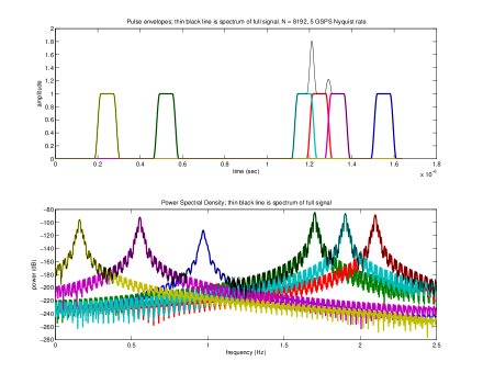
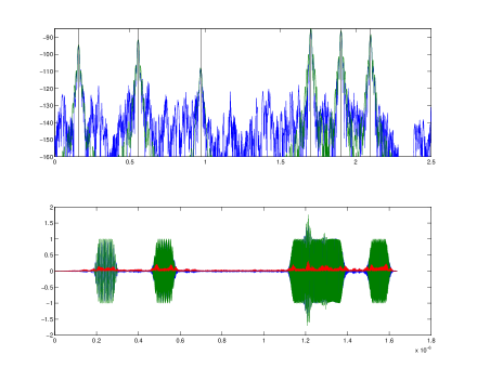
Figure 3 shows the recovery (without noise) by $\ell_{1}$-analysis in both the time and frequency domains. In the time domain we see (in red) that the difference between the actual signal and the recovered signal is small, as we do in the frequencey domain as well. These pulses together with the carrier frequencies are well recovered from a very small set of measurements.

Figure 3: Recovery in both the time (below) and frequency (above) domains by $\ell_{1}$-analysis. Blue denotes the recovered signal, green the actual signal, and red the difference between the two.

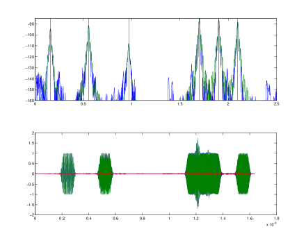
In practice, reweighting the $\ell_{1}$ norm often offers superior results. We use the reweighted $\ell_{1}$-analysis method, which solves several sequential weighted $\ell_{1}$-minimization problems, each using weights computed from the solution of the previous problem [17]. This procedure has been observed to be very effective in reducing the number of measurements needed for recovery, and outperforms standard $\ell_{1}$-minimization in many situations (see e.g. [17], [28], [33]). Figure 4 shows reconstruction results after just one reweighting iteration; the root-mean squared error (RMSE) is significantly reduced, by a factor between 3 and 4.

Figure 4: Recovery in both the time (below) and frequency (above) domains by $\ell_{1}$-analysis after one reweighted iteration. Blue denotes the recovered signal, green the actual signal, and red the difference between the two. The RMSE is less than a third of that in Figure 4

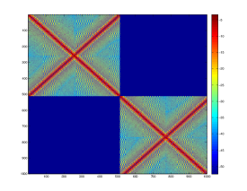
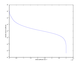
Because $D$ is massively overcomplete, the Gram matrix $D^{*}D$ is not diagonal. Figure 5 depicts part of the Gram matrix $D^{*}D$ for this dictionary, and shows that this matrix is “thick” off of the diagonal. We can observe visually that the dictionary $D$ is not an orthogonal system or even a matrix with low coherence, and that columns of this dictionary are indeed highly correlated. Having said this, the second plot in Figure 5 shows the rapid decay of the sequence $D^{*}f$ where $f$ is the signal in Figure 2.

Figure 5: Portion of the matrix $D^{*}D$, in $\log$-scale (left). Sorted analysis coefficients (in absolute value) of the signal from Figure 2 (right).

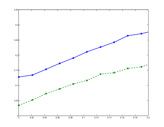
Our next simulation studies the robustness of $\ell_{1}$-analysis with respect to noise in the measurements $y=Af+z$, where $z$ is a white noise sequence with standard deviation $\sigma$. Figure 6 shows the recovery error as a function of the noise level. As expected, the relationship is linear, and this simulation shows that the constants in Theorem 1.4 seem to be quite small. This plot also shows the recovery error with respect to noise using a reweighted $\ell_{1}$-analysis; reweighting also improves performance of $\ell_{1}$-analysis, as is seen in Figure 6.

Figure 6: Relative recovery error of $\ell_{1}$-analysis as a function of the (normalized) noise level, averaged over $5$ trials. The solid line denotes standard $\ell_{1}$-analysis, and the dashed line denotes $\ell_{1}$-analysis with $3$ reweighted iterations. The $x$-axis is the relative noise level $\sqrt{m}\sigma/\|Af\|_{2}$ while the $y$-axis is the relative error $\|\hat{f}-f\|_{2}/\|f\|_{2}$.

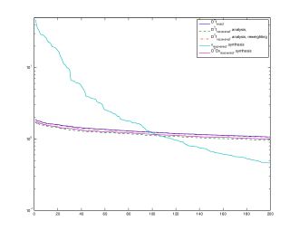
An alternative to $\ell_{1}$-analysis is $\ell_{1}$-synthesis, which we discuss in Section 4.1; $\ell_{1}$-synthesis minimizes in the coefficient domain, so its solution is a vector $\hat{x}$, and we set $\hat{f}=D\hat{x}$. Our next simulation confirms that although we cannot recover the coefficient vector $x$, we can still recover the signal of interest. Figure 7 shows the largest $200$ coefficients of the coefficient vector $x$, and those of $D^{*}f$ as well as $D^{*}\hat{f}$ for both $\ell_{1}$-analysis and $\ell_{1}$-synthesis. The plot also shows that the recovery of $\ell_{1}$-analysis with reweighting outperforms both standard $\ell_{1}$-analysis and $\ell_{1}$-synthesis.

Figure 7: The largest $200$ coefficients of the coefficient vector $D^{*}f$ (blue), $D^{*}\hat{f}$ from $\ell_{1}$-analysis (dashed green), $D^{*}\hat{f}$ from $\ell_{1}$-analysis with $3$ reweighting iterations (dashed red), $\hat{x}$ from $\ell_{1}$-synthesis (cyan), and $D^{*}\hat{f}$ from $\ell_{1}$-synthesis (magenta).

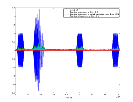
Our final simulation compares recovery error on a compressible signal (in the time domain) for the $\ell_{1}$-analysis, reweighted $\ell_{1}$-analysis, and $\ell_{1}$-synthesis methods. We see in Figure 8 that the $\ell_{1}$-analysis and $\ell_{1}$-synthesis methods both provide very good results, and that reweighted $\ell_{1}$-analysis provides even better recovery error.

Figure 8: Recovery (without noise) of a compressible signal in the time domain. Blue denotes the actual signal, while green, red, and cyan denote the recovery error from $\ell_{1}$-analysis, reweighted $\ell_{1}$-analysis ($2$ iterations), and $\ell_{1}$-synthesis, respectively. The legend shows the relative error $\|\hat{f}-f\|_{2}/\|f\|_{2}$ of the three methods.

4 Discussion

Theorem 1.4 shows that $\ell_{1}$-analysis is accurate when the coefficients of $D^{*}f$ are sparse or decay rapidly. As discussed above, this occurs in many important applications. However, if it is not the case, then the theorem does not guarantee good recovery. As previously mentioned, this may occur when the dictionary $D$ is a concatenation of two (even orthonormal) bases. For example, a signal $f$ may be decomposed as $f=f_{1}+f_{2}$ where $f_{1}$ is sparse in the basis $D_{1}$ and $f_{2}$ is sparse in a different basis, $D_{2}$. One can consider the case where these bases are the coordinate and Fourier bases, or the curvelet and wavelet bases, for example. In these cases, $D^{*}f$ is likely to decay slowly since the component that is sparse in one basis is not at all sparse in the other [19]. This suggests that $\ell_{1}$-analysis may then not be the right algorithm for reconstruction in such situations.

4.1 Alternatives

Even though $\ell_{1}$-analysis may not work well in this type of setup, one should still be able to take advantage of the sparsity in the problem. We therefore suggest a modification of $\ell_{1}$-analysis which we call Split-analysis. As the name suggests, this problem splits up the signal into the components we expect to be sparse:

$$(\hat{f}_{1},\hat{f}_{2})=\operatorname*{argmin}_{\tilde{f}_{1},\tilde{f}_{2}}\|D_{1}^{*}\tilde{f}_{1}\|_{1}+\|D_{2}^{*}\tilde{f}_{2}\|_{1}\quad\text{subject to}\quad\|A(\tilde{f}_{1}+\tilde{f}_{2})-y\|_{2}\leq\varepsilon.$$

The reconstructed signal would then be $\hat{f}=\hat{f}_{1}+\hat{f}_{2}$. Some applications of this problem in the area of image restoration have been studied in [8]. Since this is an analagous problem to $\ell_{1}$-analysis, one would hope to have a result for Split-analysis similar to Theorem 1.4.

An alternative way to exploit the sparsity in $f=f_{1}+f_{2}$ is to observe that there may still exist a (nearly) sparse expansion $f=Dx=D_{1}x_{1}+D_{2}x_{2}$. Thus one may ask that if the coefficient vector $x$ is assumed sparse, why not just minimize in this domain? This reasoning leads to an additional approach, called $\ell_{1}$-Synthesis or Basis Pursuit (see also the discussion in [21]):

$$\hat{x}=\operatorname*{argmin}_{\tilde{x}}\|\tilde{x}\|_{1}\quad\text{subject to}\quad\|AD\tilde{x}-y\|_{2}\leq\varepsilon. \ell_{1}$$ (-synthesis)

The reconstructed signal is then $\hat{f}=D\hat{x}$. Empirical studies also show that $\ell_{1}$-synthesis often provides good recovery, however, it is fundamentally distinct from $\ell_{1}$-analysis. The geometry of the two problems is analyzed in [21], and there it is shown that because these geometrical structures exhibit substantially different properties, there is a large gap between the two formulations. This theoretical gap is also demonstrated by numerical simulations in [21], which show that the two methods perform very differently on large families of signals.

4.2 Fast Transforms

For practical reasons, it is clearly advantageous to be able to use measurement matrices $A$ which allow for easy storage and fast multiplication. The partial DFT for example, exploits the Fast Fourier Transform (FFT) which allows the sampling matrix to be applied to a $n$-dimensional vector in $\mathrm{O}(n\log n)$ time, and requires only $\mathrm{O}(m\log n)$ storage. Since the partial DFT has been proven to satisfy the RIP [16] (see also [37]), it is a fast measurement matrix that can be used in many standard compressed sensing techniques.

One of course hopes that fast measurement matrices can be used in the case of redundant and coherent dictionaries as well. As mentioned, the result of Krahmer and Ward implies that any matrix which satisfies the RIP will satisfy the D-RIP when multiplied by a random sign matrix [29]. Therefore, the $m\times n$ subsampled Fourier matrix with $m=\mathrm{O}(s\log^{4}n)$ along with the sign matrix will satisfy the D-RIP and provides the fast multiply.

A result at the origin of this notion was proved by Ailon and Liberty, also after our initial submission of this paper [4]. Recall that in light of (1.5), we desire a fast transform that satisfies the Johnson-Lindenstrauss lemma in the following sense. For a set $Q$ of $N$ vectors in $n$-dimensional space, we would like a fast transform $A$ that maps this set into a space of dimension $\mathrm{O}(\log N)$ (possibly with other factors logarithmic in $n$) such that

$$(1-\delta)\|v\|_{2}^{2}\leq\|Av\|_{2}^{2}\leq(1+\delta)\|v\|_{2}^{2}\quad\text{ for all $v\in Q$.}$$ (4.1)

Note that the dimension $\mathrm{O}(\log N)$ will of course also depend on the constant $\delta$. Due to standard covering arguments (see e.g. [38, 6]), this would yield a $m\times n$ fast transform with optimal number of measurements, $m=\mathrm{O}(s\log n)$, obeying the D-RIP.

Ailon and Liberty show that the subsampled Fourier matrix multiplied by a random sign matrix does exactly this [4]. Thus in other words, for a fixed $m$, this $m\times n$ construction satisfies the D-RIP up to sparsity level $s=\mathrm{O}(m/\log^{4}n)$. The cost of a matrix–vector multiply is of course dominated by that of the FFT, $\mathrm{O}(n\log n)$. Its storage requirements are also $\mathrm{O}(m\log n)$. Their results can also be generalized to other transforms with the same type of fast multiply.

These results yield a transform with a fast multiply which satisfies the D-RIP. The number of measurements and the multiply and storage costs of the matrix are of the same magnitude as those that satisfy the RIP. The D-RIP is, therefore, satisfied by matrices with the same benefits as those in standard compressed sensing. This shows that compressed sensing with redundant and coherent dictionaries is viable with completely the same advantages as in the standard setting.

Acknowledgements

This work is partially supported by the ONR grants N00014-10-1-0599 and N00014-08-1-0749, the Waterman Award from NSF, and the NSF DMS EMSW21-VIGRE grant. EJC would like to thank Stephen Becker for valuable help with the simulations.

References

- [1] Bootstrap methods in Signal Processing. IEEE Signal Proc. Mag., 24(4), 2007.
- [2] Sensing, sampling, and compression. IEEE Signal Proc. Mag., 25(2), 2008.
- [3] N. Ailon and B. Chazelle. The fast Johnson-Lindenstrauss transform and approximate nearest neighbors. SIAM J. Comput., 39:302–322, 2009.
- [4] N. Ailon and E. Liberty. An almost optimal unrestricted fast johnson-lindenstrauss transform. Submitted, 2010.
- [5] W. Bajwa, R. Calderbank, and S. Jafarpour. Why gabor frames? two fundamental measures of coherence and their geometric significance. IEEE Trans. Sig. Proc., 2008. to appear.
- [6] R. Baraniuk, M. Davenport, R. DeVore, and M. Wakin. A simple proof of the restricted isometry property for random matrices. Constr. Approx., 28(3):253–263, 2008.
- [7] T. Blumensath and M. E. Davies. Iterative hard thresholding for compressed sensing. Appl. Comput. Harmon. Anal., 27(3):265–274, 2009.
- [8] J.-F. Cai, S. Osher, and Z. Shen. Split bregman methods and frame based image restoration. Multiscale Model. Sim., 8(2):337–369, 2009.
- [9] E. J. Candès. The restricted isometry property and its implications for compressed sensing. C. R. Math. Acad. Sci. Paris, Serie I, 346:589– 592, 2008.
- [10] E. J. Candès, L. Demanet, D. L. Donoho, and L. Ying. Fast discrete curvelet transforms. Multiscale Model. Simul., 5:861–899, 2000.
- [11] E. J. Candès and D. L. Donoho. New tight frames of curvelets and optimal representations of objects with piecewise singularities. Comm. Pure Appl. Math., 57(2):219–266, 2004.
- [12] E. J. Candès and Y. Plan. Near-ideal model selection by minimization. Ann. Stat., 37:2145–2177, 2007.
- [13] E. J. Candès, J. Romberg, and T. Tao. Robust uncertainty principles: Exact signal reconstruction from highly incomplete Fourier information. IEEE Trans. Info. Theory, 52(2):489–509, Feb. 2006.
- [14] E. J. Candès, J. Romberg, and T. Tao. Stable signal recovery from incomplete and inaccurate measurements. Communications on Pure and Applied Mathematics, 59(8):1207–1223, 2006.
- [15] E. J. Candès and T. Tao. Decoding by linear programming. IEEE Trans. Inform. Theory, 51:4203–4215, 2005.
- [16] E. J. Candès and T. Tao. Near optimal signal recovery from random projections: Universal encoding strategies? IEEE Trans. Inform. Theory, 52(12):5406–5425, Dec. 2006.
- [17] E. J. Candès, M. Wakin, and S. Boyd. Enhancing sparsity by reweighted minimization. J. Fourier Anal. Appl., 14(5):877–905, Dec. 2008.
- [18] D. L. Donoho. Compressed sensing. IEEE Trans. Info. Theory, 52(4):1289–1306, Apr. 2006.
- [19] D. L. Donoho and G. Kutyniok. Microlocal analysis of the geometric separation problem. Submitted, 2010.
- [20] P. Dutilleux. An implementation of the “algorithme à trous” to compute the wavelet transform. in Wavelets: Time-Frequency Methods and Phase-Space, J.M. Combes, A. Grossmann, and P. Tchamitchian, Eds. New York: Springer, 1989.
- [21] M. Elad, P. Milanfar, and R. Rubinstein. Analysis versus synthesis in signal priors. Inverse Probl., 23(3):947–968, 2007.
- [22] H. Feichtinger and T. Strohmer, editors. Gabor Analysis and Algorithms. Birkhäuser, 1998.
- [23] M. Fornasier and H. Rauhut. Iterative thresholding algorithms. Appl. Comput. Harmon. Anal, 25(2):187–208, 2008.
- [24] S. Foucart. A note on guaranteed sparse recovery via -minimization. Appl. Comput. Harmon. Anal., 2010. To appear.
- [25] S. Foucart and M.-J. Lai. Sparsest solutions of undetermined linear systems via -minimization for . Appl. Comput. Harmon. Anal., 26(3):395–407, 2009.
- [26] A. C. Gilbert, M. Muthukrishnan, and M. J. Strauss. Approximation of functions over redundant dictionaries using coherence. In Proc. of the 14th Annual ACM-SIAM Symposium on Discrete Algorithms, Jan. 2003.
- [27] A. Hinrichs and J. Vybiral. Johnson-lindenstrauss lemma for circulant matrices. Submitted, 2010.
- [28] A. Khajehnejad, W. Xu, S. Avestimehr, and B. Hassibi. Improved sparse recovery thresholds with two-step reweighted minimization. In IEEE Int. Symposium on Information Theory (ISIT), 2010.
- [29] F. Krahmer and R. Ward. New and improved Johnson-Lindenstrauss embeddings via the restricted isometry property. Submitted, 2010.
- [30] S. Mallat. A Wavelet Tour of Signal Processing. Academic Press, London, 2nd edition, 1999.
- [31] S. Mallat and Z. Zhang. Matching Pursuits with time-frequency dictionaries. IEEE Trans. Signal Process., 41(12):3397–3415, 1993.
- [32] S. Mendelson, A. Pajor, and N. Tomczak-Jaegermann. Uniform uncertainty principle for Bernoulli and subgaussian ensembles. Constr. Approx., 28(3):277–289, 2008.
- [33] D. Needell. Noisy signal recovery via iterative reweighted -minimization. In Proc. 43rd Ann. Asilomar Conf. Signals, Systems, and Computers, 2009.
- [34] D. Needell and J. A. Tropp. CoSaMP: Iterative signal recovery from noisy samples. Appl. Comput. Harmon. Anal., 26(3):301–321, 2008.
- [35] P. Randall. Sparse Recovery via Convex Optimization. Ph.D. dissertation, California Institute of Technology, 2009.
- [36] A. Ron and Z. Shen. Affine systems in : the analysis of the analysis operator,. J. Funct. Anal., 148:408–447, 1997.
- [37] M. Rudelson and R. Vershynin. On sparse reconstruction from Fourier and Gaussian measurements. Comm. Pure Appl. Math., 61:1025–1045, 2008.
- [38] H. Rauhut K. Schnass and P. Vandergheynst. Compressed sensing and redundant dictionaries. IEEE Trans. Inform. Theory, 54(5):2210–2219, 2008.
- [39] J.-L. Starck, M. Elad, and D.L. Donoho. Redundant multiscale transforms and their application for morphological component analysis. Adv. Imag. Elect. Phys., 132, 2004.
- [40] J.-L. Starck, J. Fadili, and F. Murtagh. The undecimated wavelet decomposition and its reconstruction. IEEE Trans. Sig. Proc., 16(2):297–309, 2007.
- [41] J. A. Tropp. Greed is good: Algorithmic results for sparse approximation. IEEE Trans. Info. Theory, 50(10):2231–2242, 2004.
- [42] J. A. Tropp and A. C. Gilbert. Signal recovery from random measurements via Orthogonal Matching Pursuit. IEEE Trans. Info. Theory, 53(12):4655–4666, 2007.