Anomalous spin Hall effects in Dresselhaus (110) quantum wells

Abstract

Anomalous spin Hall effects that belong to the intrinsic type in Dresselhaus (110) quantum wells are discussed. For the out-of-plane spin component, antisymmetric current-induced spin polarization induces opposite spin Hall accumulation, even though there is no spin-orbit force due to Dresselhaus (110) coupling. A surprising feature of this spin Hall induction is that the spin accumulation sign does not change upon bias reversal. Contribution to the spin Hall accumulation from the spin Hall induction and the spin deviation due to intrinsic spin-orbit force as well as extrinsic spin scattering, can be straightforwardly distinguished simply by reversing the bias. For the inplane component, inclusion of a weak Rashba coupling leads to a new type of $S_{y}$ intrinsic spin Hall effect solely due to spin-orbit-force-driven spin separation.

I Introduction

The intensive efforts on spin Hall effect (SHE) both experimentally and theoretically during the past decade have successfully built another milestone in condensed matter physics. Spin separation in semiconductors is not only possible but natural, so that manipulating spin properties of charge carriers in electronics is promising. The earliest theoretical idea that up and down spins may laterally separate upon transport due to asymmetric scattering was proposed in 1971.D’yakonov and Perel’ (1971, 1971) More than three decades later, the power of optical measurements on high quality mesoscopic samples made SHE in semiconductors no longer an idea but an experimental fact.Kato et al. (2004) Right before the first observation of Ref. Kato et al., 2004 in 2004, mechanisms of SHE was further extended from spin-dependent scattering that was later categorized as extrinsic, to spin-orbit-coupled band structure that was later categorized as intrinsic.Murakami et al. (2003); Sinova et al. (2004) Experimentally, most observations so far have been attributed to the extrinsic SHE,Kato et al. (2004); Sih et al. (2005); Valenzuela and Tinkham (2006); Seki et al. (2008) while evidence of the intrinsic SHEWunderlich et al. (2005) is relatively few. Nonetheless, intrinsic SHE remains an important issue that until now still receives enduring efforts.Brüne et al. (2010)

In the intrinsic SHE, spin separation is solely due to the underlying spin-orbit coupling in the band structure, so that SHE can exist even in systems free of scattering (but of finite sizesInoue et al. (2004); Chalaev and Loss (2005)). In the ballistic limit, the spin separation can be vividly visualized by the transverse spin-orbit force Li et al. (2005); Nikolić et al. (2005) derived by using the Heisenberg equation of motion,

$$\mathbf{F}_{so}=\frac{m}{i\hbar}\left[\frac{1}{i\hbar}\left[\mathbf{r},\mathcal{H}\right],\mathcal{H}\right],$$ (1)

where $\mathbf{r}$ is the position operator and $\mathcal{H}$ is the single-particle Hamiltonian. For well discussed two-dimensional systems with Rashba coupling Bychkov and Rashba (1984) described by $\mathcal{H}_{R}=\left(\alpha/\hbar\right)\left(p_{y}\sigma^{x}-p_{x}\sigma^{y}\right)$, as well as linear Dresselhaus (001) coupling Dresselhaus (1955); D’yakonov and Kachorovskii (1986) described by $\mathcal{H}_{D}^{001}=\left(\beta/\hbar\right)\left(p_{x}\sigma^{x}-p_{y}\sigma^{y}\right),$ the spin-orbit force is given by Li et al. (2005)

$$\mathbf{F}_{so}^{RD001}=\frac{2m\left(\alpha^{2}-\beta^{2}\right)}{\hbar^{3}}\left(\mathbf{p}\times\mathbf{e}_{z}\right)\sigma^{z},$$ (2)

where $\mathbf{p}$ is the momentum and $\mathbf{e}_{z}$ is the unit vector of the plane normal. Here $\alpha$ and $\beta$ are Rashba and Dresselhaus coupling constants, respectively, and $\sigma^{x},\sigma^{y},\sigma^{z}$ are Pauli matrices. Equation (2) clearly depicts a lateral spin deviation of the $S_{z}=(\hbar/2)\sigma^{z}$ spin component with opposite contributions from Rashba and Dresselhaus (001) couplings, as sketched in Fig. 1(a) and (b), respectively.

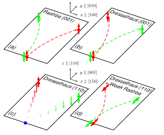
Figure 1: (Color online) Spin deviation in $S_{z}$ due to spin-orbit force in (a) Rashba and (b) linear Dresselhaus [001] systems. (c) Spin Hall induction due to antisymmetric CISP along [001̄] in Dresselhaus [110] systems may cause opposite $S_{z}$ accumulations as well, even though there is no spin-orbit force. (d) In the case of linear Dresselhaus [110] plus weak Rashba couplings, a coupled spin-orbit force given by Eq. (11) may lead to spin deviation in $S_{y}$.

SHE in Dresselhaus (110) quantum wells (QWs), on the other hand, is relatively less discussed theoretically,Hankiewicz et al. (2006) although a previous experimental effort Sih et al. (2005) had revealed in GaAs (110) QWs the existence of SHE that was attributed to the extrinsic type. In this paper, anomalous SHEs that belong to the intrinsic type in Dresselhaus (110) QWs are discussed. We show that the spin Hall pattern of $S_{z}$ can be induced when the transport direction is properly oriented, even though the Dresselhaus (110) coupling does not result in spin-orbit force to separate opposite $S_{z}$ spins upon transport [see Fig. 1(c)]. Moreover, we propose a Rashba-coupling-assisted intrinsic SHE in $S_{y}$ that is truly due to spin-orbit force under the interaction of Dresselhaus (110) plus a weak Rashba couplings [Fig. 1(d)].

This paper is organized as follows. In Sec. II we briefly introduce the formulas required in the Landauer-Keldysh formalism employed in the numerical analysis of Sec. III, where we visualize the proposed spin Hall induction and Rashba-coupling-assisted SHE in $S_{y}$. Comparison of the present ballistic calculation with the diffusive experiment of Ref. Sih et al., 2005 will be discussed and the transport parameters used in our numerical data will be remarked. We conclude in Sec. IV.

II Formulas

II.1 Linear Dresselhaus (110) coupling

The Dresselhaus (110) coupling up to the term linear in momentum can be written as

$$\mathcal{H}_{D}^{110}=-\frac{\beta}{\hbar}p_{x}\sigma^{z},$$ (3)

where $x$, $y$, and $z$ axes are chosen along [11̄0], [001̄], and [110], respectively. Throughout the present discussion, we will focus on this Dresselhaus (110) linear term, so that without ambiguity we use the same notation $\beta$ to denote its coupling strength. The spin-orbit field subject to Eq. (3) is depicted in Fig. 2(a). Clearly, when propagating with $\mathbf{k}=\left(\pm\left|k_{x}\right|,k_{y}\right)$ electrons encounter antisymmetric spin-orbit fields on the left and right sides of the [001̄] axis (or the $y$ axis). Hence the current-induced spin polarization (CISP) effect Edelstein (1990); Kato et al. (2004); Liu et al. (2008) is expected to build opposite $S_{z}$ spin densities at the two sides, as conceptually depicted in Fig. 1(c).

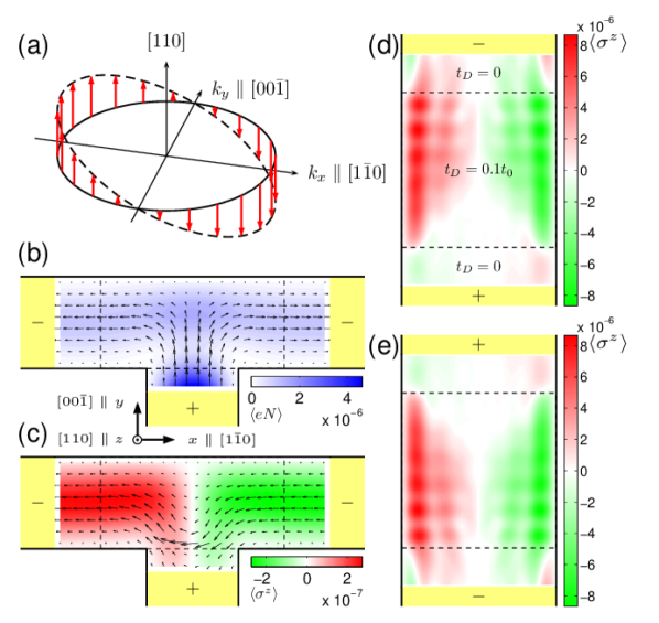
Figure 2: (Color online) (a) Linear Dresselhaus [110] spin-orbit field in $k$ space. (b) Local charge density $\langle eN\rangle$ (color shading) and local charge current density (arrows) in a $16a\times 8a$ Dresselhaus [110] sample subject to three terminals with a weak bias $eV_{0}=10^{-3}t_{0}$. (c) Local spin density $\langle\sigma^{z}\rangle$ (color shading) and its corresponding local spin current density $\langle\mathbf{J}^{S_{z}}\rangle$ (arrows) in the same device as (b) with same conditions. Spin Hall induction in a $40a\times 40a$ Dresselhaus [110] sample with (d) upward bias and (e) downward bias; strong bias $eV_{0}=0.4t_{0}$ is applied. Note that in (b)–(e), the regions outside the dashed lines are simulating the leads (zero spin-orbit coupling and constant on-site energy set equal to the applied bias).

To better illustrate this spin Hall induction, we will in Sec. III first consider a T-bar ballistic nanostructure, attached to left, right, and bottom leads (from the top view) that are made of normal metals. The central region is described by the square-lattice tight-binding Hamiltonian,

$$H=\left(U+4t_{0}\right)\openone\sum_{n}c_{n}^{{\dagger}}c_{n}+\sum_{\langle nm\rangle}c_{m}^{{\dagger}}\mathbf{t}_{m\leftarrow n}c_{n},$$ (4)

where the sum over $\langle nm\rangle$ of the second term is run for the sites nearest to each other, satisfying $\left|\mathbf{r}_{m}-\mathbf{r}_{n}\right|=a,$ $a$ being the lattice grid spacing and $\mathbf{r}_{n}$ the position vector of site $n$, and the hopping matrix is given by

$$\mathbf{t}_{m\leftarrow n}=-t_{0}\openone-it_{D}d_{x}\sigma^{z}.$$ (5)

Here $U$ is the on-site energy set to be constant over the whole sample, $t_{0}=\hbar^{2}/2ma^{2}$ is the kinetic hopping energy, $\openone$ is the identity, $c_{m}$ ($c_{m}^{{\dagger}}$) annihilates (creates) an electron at site $m$, $t_{D}=\beta/2a$ is the Dresselhaus hopping parameter, and $d_{x}=\left(\mathbf{r}_{m}-\mathbf{r}_{n}\right)\cdot\mathbf{e}_{x}$ is the hopping displacement along $x$ from site $m$ to site $n$.

II.2 Landauer-Keldysh formalism

To image the nonequilibrium charge, charge current, spin, and spin current densities under the influence of the biased leads, a powerful and convenient approach is the Landauer-Keldysh formalism,Nikolić et al. (2005); Datta (1995) especially for the present ballistic case free of particle-particle interaction. In this formalism, physical quantities in a nonequilibrium but steady state are expressed in terms of the lesser Green function matrix $G^{<}$, provided that those physical observables of interest are well defined.Nikolić et al. (2006) Each matrix element $G_{mn}^{<}$ in our spin-1/2 electron system is a $2\times 2$ submatrix, so that the size of full $G^{<}$ amounts to $2N\times 2N$, $N$ being the total number of lattice grid points. Following Ref. Nikolić et al., 2006 with moderate extension, we have and will use the local charge and spin densities

$$\langle eN_{n}\rangle = \frac{e}{2\pi i}\int dE\mathop{\mathrm{T}r}_{s}G_{nn}^{<}$$ (6)

$$\frac{\hbar}{2}\langle\sigma_{n}^{i}\rangle = \frac{\hbar/2}{2\pi i}\int dE\mathop{\mathrm{T}r}_{s}\left[\sigma^{i}G_{nn}^{<}\right]$$ (7)

for site $n$, and the local charge and spin current densities

$$\langle J_{n\rightarrow m}\rangle = -\frac{e}{h}\int dE\mathop{\mathrm{T}r}_{s}\left[\mathbf{t}_{m\leftarrow n}G_{nm}^{<}-\mathbf{t}_{n\leftarrow m}G_{mn}^{<}\right]$$ (8)

$$\langle J_{n\rightarrow m}^{S_{i}}\rangle = -\frac{1}{8\pi}\int dE\mathop{\mathrm{T}r}_{s}[\left\{\mathbf{t}_{m\leftarrow n},\sigma^{i}\right\}G_{nm}^{<}$$ (9)

$$-\left\{\mathbf{t}_{m\leftarrow n}^{{\dagger}},\sigma^{i}\right\}G_{mn}^{<}]$$

for the flow from site $n$ to site $m$. Here $\mathop{\mathrm{T}r}_{s}$ is the trace done in the spin space, the explicit energy $E$ dependence of $G_{mn}^{<}\left(E\right)$ is suppressed, and $\left\{A,B\right\}=AB+BA$ is the anticommutator. For the present illustration of the spin Hall induction, we will first consider a pure linear Dresselhaus (110) system and use the hopping matrix (5) with $t_{D}=0.1t_{0}$, which is within a reasonable range. Parameters extracted from experiments will be discussed later in Sec. III.4. Other transport parameters are as follows: hopping parameter $t_{0}=1,$ on-site energy $U=0$ (so that band bottom $E_{b}=0$), Fermi energy is $0.2t_{0}$ above $E_{b}$ (so that the square lattice simply serves as the grid of a free electron gas). We will always label $+$ and $-$ to indicate an applied bias voltage of $+eV_{0}/2$ and $-eV_{0}/2$ on each lead, respectively, with $eV_{0}>0$. (Note that $e=-\left|e\right|$ is the negative electron charge, and hence electrons always flow from $+$ to $-$ signs). In the rest of our analysis, we will focus on the nonequilibrium contribution Nikolić et al. (2006) of those quantities listed in Eqs. (6)–(9), and hence the integration range will be taken as $E_{F}-eV_{0}/2\rightarrow E_{F}+eV_{0}/2$.

III Numerical Analysis

III.1 Spin Hall induction in $S_{z}$: Pure Dresselhaus (110) coupling

Employing the Landauer-Keldysh formalism briefly introduced above, we now drive electrons in the T-bar nanostructure from bottom to left and right leads with $eV_{0}=10^{-3}t_{0}$, as shown in Fig. 2(b), where the background color shading is determined by the local charge density $\langle eN\rangle$ given in Eq. (6), while each arrow indicates the local charge current density given by Eq. (8). In Fig. 2(c), the color shading is determined by the local spin $\langle S_{z}\rangle$ density [Eq. (7)] and clearly shows an antisymmetric $S_{z}$ polarization for electrons moving into the left and right leads because of the opposite Dresselhaus (110) fields they feel. The local spin current density indicated by the arrows therein is given by Eq. (9), which is derived from the symmetrized spin current operator $J^{S_{i}}=\left\{J_{m\rightarrow n}/e,S_{i}\right\}/2$ in a way similar to Ref. Nikolić et al., 2006. A pure spin current from right to left is observed; at right side the spin current is flowing toward left because of the negative $S_{z}$ times the right moving particle current while at left side the left flowing spin current stems from the product of the positive $S_{z}$ and the left moving particle current.

For a two-terminal device made of Dresselhaus (110) QW oriented along [001̄] ($y$ axis), spin Hall accumulation of opposite $S_{z}$ is therefore expected, as shown in Fig. 2(d)–(e), where we consider a strong bias voltage of $eV_{0}=0.4t_{0}$ for a $40a\times 40a$ sample. A striking difference between the spin Hall induction introduced here and the spin Hall deviation due to spin-orbit force is the independence of the accumulation sign on the bias direction. Whether driving the electrons from bottom to top [Fig. 2(d)] or from top to bottom [Fig. 2(e)], one always observe a negative $S_{z}$ accumulation at right while positive at left.

Contrary to the present ballistic nanostructure here, the SHE previously observed in GaAs (110) QWs Sih et al. (2005) was in diffusive regime and attributed to the extrinsic type. The experiment used ac lock-in detection referenced to the frequency of a square wave alternating voltage with zero dc bias offset, and the resulting signal is sensitive only to the difference in Kerr rotation between positive and negative bias. Our spin Hall induction that does not depend on bias direction may therefore either hardly contribute or be subtracted in the result of Ref. Sih et al., 2005.

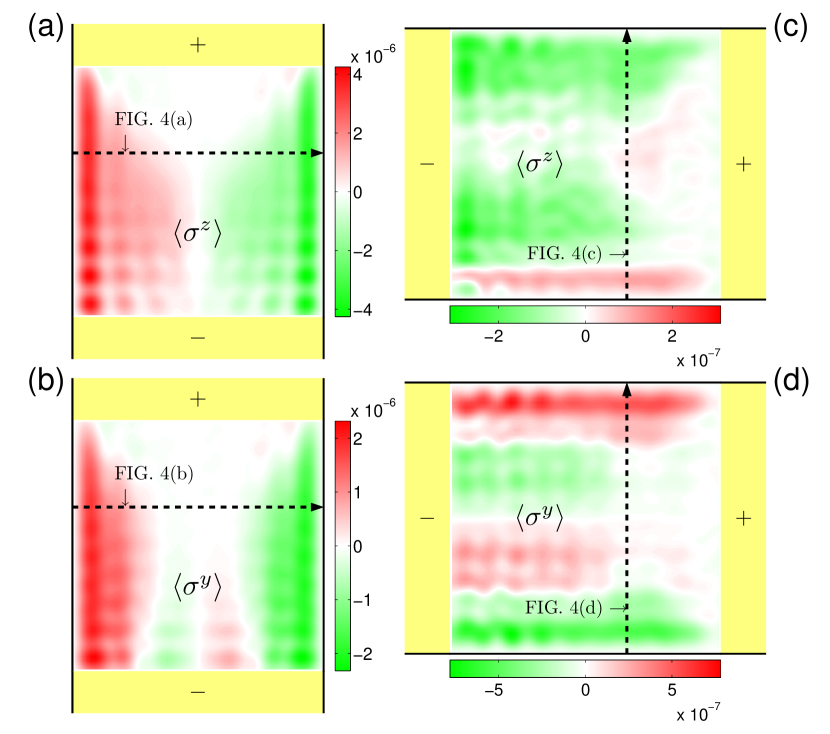
Figure 3: (Color online) Imaging of local spin densities $\langle\sigma^{z}\rangle$ and $\langle\sigma^{y}\rangle$ in a $60a\times 60a$ [110] sample with (a)–(b) top-to-bottom and (c)–(d) right-to-left orientations. A strong Dresselhaus [110] coupling $t_{D}=0.08t_{0}$ and a weak Rashba coupling $t_{R}=0.02t_{0}$ are used. Bias is set $eV_{0}=0.4t_{0}$.

III.2 Spin Hall deviation in $S_{y}$: Strong Dresselhaus (110) with weak Rashba couplings

Next we recall the spin-orbit force Eq. (1). For pure Dresselhaus (110) systems given by Eq. (3), there is no way to obtain a nonvanishing $\mathbf{F}_{so}$ since eventually the Pauli matrix $\sigma^{z}$ will commute with itself, even if the cubic term that is still in terms of $\sigma^{z}$ is involved. The only possibility in this case for a nonvanishing $\mathbf{F}_{so}$ to survive is to introduce spin-orbit terms involving $\sigma^{x}$ or $\sigma^{y}$. Combination of Rashba coupling with the present linear Dresselhaus (110) term is therefore a natural candidate, which is possible for, for example, asymmetric GaAs (110) QWs, as are the cases of Ref. Sih et al., 2005. The spin-orbit force for this Rashba-Dresselhaus (110) QW is

$$\mathbf{F}_{so}^{RD110}=\frac{2m\alpha}{\hbar^{3}}\left(\mathbf{p}\times\mathbf{e}_{z}\right)\left(\alpha\sigma^{z}-\beta\sigma^{y}\right).$$ (10)

Without Rashba term $\alpha,$ the spin-orbit force vanishes and zero spin current is hence expected. From a gauge viewpoint, the existence of equilibrium spin current in (110) QWs will require Rashba term to break the pure gauge.Tokatly and Sherman (2010) Note also that the $\alpha$ squared dependence for the $\sigma^{z}$ component in Eq. (10) is similar to the result in Ref. Sherman et al., 2005.

Here of particular interest is the case of weak Rashba coupling, such that Eq. (10) becomes

$$\left.\mathbf{F}_{so}^{RD110}\right|_{\alpha\ll\beta}\approx-\frac{2m\alpha\beta}{\hbar^{3}}\left(\mathbf{p}\times\mathbf{e}_{z}\right)\sigma^{y},$$ (11)

which predicts a lateral spin Hall deviation in $S_{y}$ that requires a weak but nonzero Rashba coupling $\alpha$. To further visualize the predicted Rashba-assisted $S_{y}$ SHE, we consider a $60a\times 60a$ sample with Dresselhaus (110) hopping $t_{D}=0.08t_{0}$ and Rashba hopping $t_{R}\equiv\alpha/2a=0.02t_{0}$, attached to two leads under a bias voltage $eV_{0}=0.4t_{0}$. For the [001]-oriented (electron flow along $-y$) sample, the $S_{z}$ spin Hall pattern due to spin Hall induction is observed in Fig. 3(a). Meanwhile, an $S_{y}$ spin Hall pattern is also shown in Fig. 3(b), which is a combined consequence of not only the spin deviation Eq. (11) but also an antisymmetric CISP by the Rashba coupling. Along the $-y$ axis, electrons with wave vector $\mathbf{k}=\left(\pm\left|k_{x}\right|,-\left|k_{y}\right|\right)$ encounter opposite $y$ component of the clockwise Rashba spin-orbit field: negative for $+\left|k_{x}\right|$ and positive for $-\left|k_{x}\right|$. Hence a spin Hall induction in $S_{y}$ due to Rashba coupling contributes to Fig. 3(b) as well. In addition, the contribution of the spin-orbit force Eq. (11) predicts a $+S_{y}$ ($-S_{y}$) accumulation at left (right) side of the electron flow, for lateral distance shorter than the spin precession length $L_{so}$ (around $15a$ here); the accumulation sign reverses when the lateral distance exceeds $L_{so}$, as is the case in our $60a\times 60a$ here. Therefore the two contributions, spin Hall induction and spin-orbit force Eq. (11), are additive in Fig. 3(b).

For the [1̄10]-oriented (electron flow along $-x$) sample, there is a vague spin Hall pattern in $S_{z}$ because of the absence of the antisymmetric CISP and weak spin-orbit force [Fig. 3(c)]. The average of $\langle S_{z}\rangle$ over the whole sample basically reveals the usual CISP effect as observed in Ref. Sih et al., 2005. The $S_{y}$ pattern, on the other hand, exhibits a clear spin Hall accumulation pattern which is solely attributed to the spin-orbit force Eq. (11), as shown in Fig. 3(d). As explained, $-S_{y}$ ($+S_{y}$) accumulates at left (right) side of the electron flow because the lateral distance has exceeded $L_{so}$. Upon the bias reversal, the $\pm S_{y}$ edge accumulations swap (not shown here), which is the general feature of the spin Hall pattern due to spin deviation by intrinsic spin-orbit force, as well as by extrinsic spin scattering. The spin Hall induction such as that of $S_{z}$ in the Dresselhaus (110) case along $\pm y$, however, does not have this feature. Another difference between the spin Hall patterns induced by antisymmetric CISP and spin-orbit-driven spin deviation is that in the former the signs of the spin accumulation do not change with the increasing sample width, while in the latter they do. This difference can also be told in Fig. 3: constant sign in each lateral side in panel (a) but varying sign in panels (b) and (d).

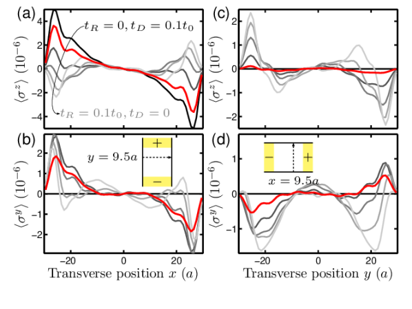
Figure 4: (Color online) Local spin densities $\langle\sigma^{z}\rangle$ and $\langle\sigma^{y}\rangle$ in a $60a\times 60a$ sample as a function of the transverse position with various coupling parameters $t_{D}$ and $t_{R}$. The origin is set at the center of the sample. As indicated in panel (a), the coupling parameters from black to the lightest curves are $\left(t_{R},t_{D}\right)=\left(0,0.1\right)t_{0},$ $\left(0.02,0.08\right)t_{0},$ $\left(0.04,0.06\right)t_{0},$ $\left(0.06,0.04\right)t_{0},$ $\left(0.08,0.02\right)t_{0},$ and $\left(0.1,0\right)t_{0}$. In each panel, the red (dark gray) thick curve correspond to Fig. 3.

III.3 From pure Dresselhaus (110) to pure Rashba cases

Finally, we laterally scan the local spin densities $\langle S_{z}\rangle$ and $\langle S_{y}\rangle$ in Fig. 4 at the positions marked by the dashed lines in Fig. 3, for a set of various spin-orbit coupling parameters from pure Dresselhaus (110) (black curves) to pure Rashba (lightest gray curves). For the [001]-oriented sample, $S_{z}$ spin Hall pattern shown in Fig. 4(a) gradually evolves from spin Hall induction due to Dresselhaus (110) coupling to spin Hall deviation driven by spin-orbit force due to Rashba coupling. In Fig. 4(b), the black curve for the pure Dresselhaus (110) shows zero everywhere [and so are those for Fig. 4(c)–(d)], while a weak Rashba coupling assists the formation of the $S_{y}$ spin Hall pattern; the antisymmetric pattern holds all the way to pure Rashba because the Rashba coupling contributes through the antisymmetric CISP in this orientation as explained previously. For the [1̄10]-oriented sample, turning on of the weak Rashba coupling builds $S_{y}$ spin Hall pattern [Fig. 4(d)] but not too much for $S_{z}$ [Fig. 4(c)]. Down to pure Rashba, the $S_{z}$ pattern recovers the spin Hall accumulation due to spin-orbit force [Fig. 4(c)], while that for $S_{y}$ shows symmetric CISP [Fig. 4(d)].

III.4 Remark on transport parameters

In our numerical analysis for the pure Dresselhaus case, we have set $t_{D}/t_{0}=0.1$ mostly based on an illustrative reason. This coupling ratio allows a direction comparison with Ref. Nikolić et al., 2005, where $t_{R}/t_{0}=0.1$ is chosen, in the later part of coexisting Rashba and linear Dresselhaus (110) couplings (such as Fig. 4).

Comparing with the GaAs (110) QWs used in the experiment of Ref. Sih et al., 2005, the coupling ratio $t_{D}/t_{0}$ may be one order weaker than ours. The sample they used behaves like a single $75\unit{\text{\AA}}$ Al_0.1Ga_0.9As QW. Using the relation $\beta=\gamma\langle k_{z}^{2}\rangle$ with hard wall approximation $\langle k_{z}^{2}\rangle\approx\left(\pi/w\right)^{2}$ and $\gamma\approx 27\unit{eV}\unit{\text{\AA}}^{3}$ for both GaAs and InAs QWs,Winkler (2003) this well width of $w=75\unit{\text{\AA}}$ leads to $\beta\approx 4.74\times 10^{-2}\unit{eV}\unit{\text{\AA}}$. Effective mass was reported to be $m=0.074m_{0}$, $m_{0}$ the electron rest mass. The sheet density is $n_{s}=1.9\times 10^{12}\unit{cm}^{-2},$ which allows us to estimate the location of the Fermi energyDatta (1995) $E_{F}-E_{b}=\pi\hbar^{2}n_{s}/m\approx 6.\,\allowbreak 15\times 10^{-2}\unit{eV}$. In order for the long wavelength limit to be valid, the chosen lattice constant $a$ has to yield a kinetic hopping constant $t_{0}$ that keeps $E_{F}$ close to $E_{b}$. Choosing $a=2\unit{nm}$ leads to $t_{0}\approx 0.13\unit{eV}$ so that $E_{F}-E_{b}\approx 0.12t_{0}$ is satisfying (recall $E_{F}-E_{b}=0.2t_{0}$ in our numerical results as well as in Refs. Nikolić et al., 2005, 2006). The coupling ratio with this $a$ is $t_{D}/t_{0}\approx 0.01.$ The Rashba strength in Ref. Sih et al., 2005 was reported to be $\alpha=0.018\unit{eV}\unit{\text{\AA}}$, leading to $\alpha/\beta\approx 0.38$, which is not too far from our $t_{R}/t_{D}=0.25$ in Sec. III.2. Replacing these parameters in our results does not change significantly the main features we have shown.

Coupling ratio of $t_{D}/t_{0}=0.1$ is actually possible for QWs with stronger Dresselhaus bulk coefficient $\gamma$. For InSb QWs,Winkler (2003) we have $\gamma=760\unit{eV}\unit{\text{\AA}}^{3}$. Consider the In_0.89Ga_0.11Sb QWs with effective mass $m=0.018m_{0}$ and sheet electron concentration $n_{s}=2.9\times 10^{11}\unit{cm}^{-2}$ reported in Ref. Akabori et al., 2008, where the QW width is relatively thick: $30\unit{nm}$. If reducing the QW width to $7.5\unit{nm}$, which is common in GaAs QWs, and assuming $a=3\unit{nm}$, the coupling ratio is estimated as $t_{D}/t_{0}\approx 9.\,\allowbreak 45\times 10^{-2}$, close to our $t_{D}/t_{0}=0.1$. The Fermi energy in units of $t_{0}$ is $(E_{F}-E_{b})/t_{0}=2\pi a^{2}n_{s}\approx 0.16$, which is also close to our $(E_{F}-E_{b})/t_{0}=0.2$. Hence the transport parameters used in our calculation are within a reasonable range.

Table 1: Effective mass and Dresselhaus coefficients taken from Ref. Winkler, 2003.

QW type	GaAs	AlAs	InAs	InSb	CdTe	ZnSe
$m/m_{0}$	$0.067$	$0.15$	$0.023$	$0.014$	$0.09$	$0.16$
$\gamma(\unit{eV}\unit{\text{\AA}}^{3})$	$27.58$	$18.53$	$27.18$	$760.1$	$43.88$	$14.29$

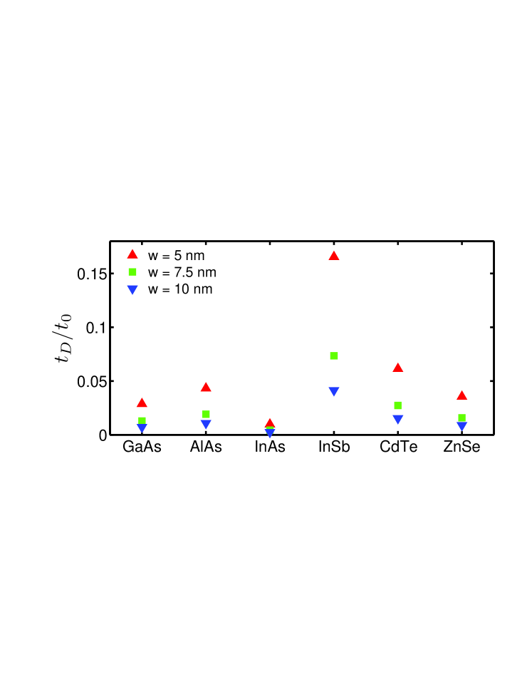
Figure 5: (Online color) Coupling ratios $t_{D}/t_{0}$ estimated by Eq. (12) for various QWs with widths $w=5\unit{nm},7.5\unit{nm},10\unit{nm}$.

In general for a stronger $t_{D}/t_{0}$, which can be rewritten as

$$\frac{t_{D}}{t_{0}}=\frac{\beta/2a}{\hbar^{2}/2ma^{2}}\approx\frac{am\gamma}{\hbar^{2}}\left(\frac{\pi}{w}\right)^{2},$$ (12)

a larger product $m\gamma$, and a thinner QW width $w$ will be required. The effective mass $m$ and Dresselhaus coefficient $\gamma$ for various QWs taken from Ref. Winkler, 2003 are collected in Table 1. For these QWs we use Eq. (12) with $a=3\unit{nm}$ to summarize the coupling ratio $t_{D}/t_{0}$ in Fig. 5 for QW widths $w=5\unit{nm},7.5\unit{nm},10\unit{nm}$.

IV Conclusion

In conclusion, we have shown that spin Hall induction for $\pm[001]$ transport in (110) QWs due to antisymmetric CISP of linear Dresselhaus coupling that yields zero spin-orbit force is possible to generate a spin Hall accumulation pattern in $S_{z}$, whose signs do not depend on the bias direction. Experimental investigations with a dc bias offset in ballistic (or at least quasi-ballistic) III-V (110) symmetric QWs may potentially identify our proposed effect. From the coupling ratios summarized in Fig. 5, InSb (110) QW is promising for the presently proposed spin Hall induction in $S_{z}$, while InAs is less suggested. A new type of spin Hall deviation in $S_{y}$ is also predicted in the Dresselhaus (110) QWs in the presence of a weak Rashba coupling. Experimental observation for this $S_{y}$ spin Hall effect may require a good control over the Rashba and Dresselhaus couplings, which has been proved possible for (001) QWs,Ganichev et al. (2004); Meier et al. (2007); Koralek et al. (2009) and should be achievable also for (110) QWs. We categorize these two intrinsic spin Hall mechanisms—spin Hall induction in $S_{z}$ and spin Hall deviation in $S_{y}$, as anomalous SHEs.

We note that the Dresselhaus cubic term, neglected in the present study, will become important when Fermi wave vector $k_{F}$ is long or QW width $w$ is thick. In this case the spin Hall induction in $S_{z}$ along $\pm$[001] axis as discussed above should remain, while additional spin Hall induction axes close to [11̄1] and [1̄12] will further emerge; see Fig. 6.20 in Ref. Winkler, 2003 and Fig. 2(a) in Ref. Sih et al., 2005. Inclusion of the Dresselhaus cubic term is left as a future extending work.