The Rest-frame Ultraviolet Light Profile Shapes of Ly$\alpha$–Emitting Galaxies at $z=3.1$

Abstract

We present a morphological analysis of the rest-frame ultraviolet emission of 78 resolved, high signal-to-noise $z\sim 3.1$ Lyman Alpha Emitters (LAEs) in the Extended Chandra Deep Field South (ECDF-S). Using HST/ACS $V$-band images taken as part of the Galaxy Evolution from Morphology and SEDS (GEMS), Great Observatories Origins Deep Survey (GOODS), and Hubble Ultra Deep Field (HUDF) surveys, we investigate both single component and multi-component LAEs, and derive concentration indices, Sérsic indices, ellipticities, and half-light radii for all resolved components and systems with a signal-to-noise $S/N>30$. We show that, although the LAE population is heterogeneous is nature, most Ly$\alpha$ emitters highly concentrated, with a distribution of $C$ values similar to that measured for field stars; this suggests that the diagnostic is a poor discriminator near the resolution limit. The LAEs also display a wide range of Sérsic indices ($0<n<12$), similar to that seen for galaxies in the local neighborhood. However, the majority of LAEs have $n<2$, and a visual inspection of the images suggests that the small$-n$ objects have extended or multimodal luminosity profiles, while the LAEs with $n>2$ have compact components surrounded by diffuse emission. Moreover, unlike nearby spiral galaxies, whose distribution of ellipticities is flat, the LAE ellipticity distribution peaks near $1-b/a\sim 0.55$. Thus, the population has more in common with $z\sim 3$ Lyman-break galaxies than local star-forming objects.

1 Introduction

In the local universe, most galaxies fall onto the Hubble Sequence (Hubble 1936) which runs from older, red, quiescent galaxies with a $r^{1/4}$ surface-brightness profiles to star-forming, gas-rich disks with exponential luminosity distributions. These light profiles are generally described by the Sersic (1968) parameter, defined through $I(r)\propto r^{1/n}$, where $n$ typically ranges from $\sim 1$ (an exponential disk) to $\sim 4$ (an r^1/4-law spheroid). Out to intermediate ($z\sim 1.5$) redshifts, galaxies can generally be placed onto the local Hubble Sequence quite reliably (Conselice et al. 2004). However, at larger distances, this sequence breaks down, as most sources appear clumpy and irregular (e.g., Steidel et al. 1996; Papovich et al. 2005; Conselice et al. 2005; Venemans et al. 2005; Pirzkal et al. 2007) and are therefore difficult to classify. Consequently, although the morphological parameters of distant galaxies can be quantified via the use of codes such as GALFIT (Peng et al. 2002) and GIM2D (Simard 1998), these parameters do not necessarily directly translate into the familiar Hubble sequence seen in the nearby universe. Moreover, the robustness of the derived parameters is highly dependent on the signal-to-noise ($S/N$) of the measurement, with simulations suggesting that a $S/N$ of at least 15 is required (Ravindranath et al. 2006) to reliably fit a high-redshift galaxy.

To address some of these difficulties, a number of non-parametric measures of galaxy morphology have been developed, including the concentration, asymmetry, and clumpiness indices (CAS; Conselice 2003), and the Gini coefficient, which measures a profile’s departure from uniformity (Lotz et al. 2004). These systems have been used extensively on samples of high-redshift galaxies, since they require no a priori knowledge about the functional form of the luminosity distribution. In addition, unlike other fitting techniques which use smooth two-dimensional profiles, these non-parametric techniques can also quantify the non-uniformity of a galaxy (i.e., test for the presence of star-forming regions), and define its asymmetry. Their one drawback, of course, is that the values one obtains may depend on the image depth, and that this sensitivity has not been well-quantified for high-redshift galaxies.

The majority of galaxies known at high ($z\geq 2.5$) redshifts have been identified via the Lyman-break technique, wherein galaxies with Lyman-limit discontinuities are identified by their unique location in color-color space (Steidel et al. 1996). Morphological analyses of these Lyman Break Galaxies (LBGs) in the rest-frame UV have revealed that most of these systems are disturbed and disk-like (i.e., with exponential profiles), and only $\sim 30\%$ have profiles consistent with galactic spheroids (e.g., Ferguson et al. 2004; Lotz et al. 2006; Ravindranath et al. 2006). Moreover, Ravindranath et al. (2006) have found that the distribution of ellipticities derived from GALFIT are skewed towards higher values, and that this asymmetry becomes more pronounced at higher redshift. This dominance of “elongated” morphologies seen in LBGs has been interpreted as evidence for galaxy formation within filamentary structure or the presence of proto-bars that span the entire visible disk of the galaxy.

Ly$\alpha$ Emitters(LAEs) are a class of high-redshift galaxies which have not been studied as extensively as LBGs. Like their Lyman break counterparts, LAEs between $2<z<4$ are actively star-forming objects (e.g., Cowie & Hu 1998), and at the bright end, the sample of LAEs overlaps that of LBGs. However, a typical Ly$\alpha$ emitting galaxy has a lower stellar mass ($\sim 10^{9}M_{\sun}$), higher mass-specific star-formation rate ($\sim 10^{-8}M_{\sun}$ yr${}^{-1}M_{\sun}^{-1}$, and lower dust content ($E(B-V)\sim 0.1$) (Venemans et al. 2005; Gawiser et al. 2007; Lai et al. 2008) than any galaxy discovered via the Lyman-break technique. Moreover, LAEs are less clustered than LBGs, suggesting a lower dark-matter halo mass, and their bias factor $b\sim 1.7$) consistent with that expected from the progenitors of present-day $L^{*}$ galaxies (Gawiser et al. 2007; Guaita et al. 2009).

To date, relatively few LAEs have been studied morphologically. In the rest-frame UV, most $3\lesssim z\lesssim 6$ LAEs are small ($\lesssim 1$ kpc), compact ($C>2.5$), and barely resolved at HST resolution (Venemans et al. 2005; Pirzkal et al. 2007; Overzier et al. 2008; Taniguchi et al. 2009). Those LAEs that are not compact ($\sim 20-45$%) exhibit clumpy or irregular morphology, with diffuse components extending to several kiloparsecs. Due to their small sizes and low luminosities, however, categorizing these objects within the context of existing classification schemes has been difficult.

Here we present a study of the rest-frame ultraviolet morphology of a statistically-complete sample of $z=3.1$ LAEs (Gronwall et al. 2007) present on archival HST/ACS $V$-band images from the Galaxy Evolution from Morphology and SEDS (GEMS, Rix et al. 2004), Great Observatories Origins Deep Survey (GOODS, Giavalisco et al. 2004), and Hubble Ultradeep Field (HUDF, Beckwith et al. 2006) surveys. In Paper I (Bond et al. 2009), we investigated the size distribution of LAEs by developing an analysis pipeline which identifies each component of an LAE, and measures its size and brightness. We found that most LAEs are extremely compact, with half-light radii, $r_{e}<2$ kpc, and that a $S/N>30$ is required for a robust measure of morphology. Here, we extend this study, and provide more detailed morphological information on each object. In § 2 and 3, we describe the data and detail the algorithms used in our morphology-fitting pipeline analysis. In § 4, we present the best-fitting morphological parameters for each galaxy, and explore how these parameters vary with image depth. Finally, in § 5, we discuss the implications of our findings. Throughout this paper, we will assume a concordance cosmology with $H_{0}=71$ km s^-1 Mpc^-1, $\Omega_{m}=0.27$, and $\Omega_{\lambda}=0.73$ (Spergel et al. 2007). With these values, $1\arcsec=7.75$ physical kpc at $z=3.1$.

2 Data

Our study uses the statistically complete sample of $z=3.1$ LAEs identified by Gronwall et al. (2007) in their narrow-band 4990 Å survey of the Extended Chandra Deep Field-South; these objects are defined to have emission-line fluxes $F_{4990}>1.5\times 10^{-17}$ ergs cm^-2 s^-1 and observed-frame Ly$\alpha$ equivalent widths EW$>80$ Å. As explained in Paper I, the sample contains $154$ LAEs in a 0.32 deg² area of sky, and $116$ of the objects fall in fields observed by HST. A full description of the data is given in Paper I (see Table I in Paper I), but to summarize: the GEMS survey includes $97$ LAEs and reaches a $V$-band $5\sigma$ point-source depth of $28.3$ mag, the GOODS survey (Version 2.0) contains $29$ LAEs and goes to a point-source depth of $V=28.8$, and HUDF contains $3$ LAEs and reaches a depth of $V=30.2$. In addition, the GEMS survey includes the first epoch of GOODS observations (reduced using their pipeline, hereafter sGOODS), and this sGOODS data reaches a depth of $V=27.9$. We note that 22/29 of our GOODS LAEs are also covered by sGOODS, 9 of the GOODS LAEs are also in GEMS, and all 3 LAEs in the HUDF are also part of GOODS. This overlaps allows us to test the depth-dependence of some of our morphological diagnostics.

We retrieved $V_{606}$-band ACS images from the Multimission Archive at the Space Telescope Science Institute. We chose $V$ for our study, in order to use the GEMS frames (which are $V$-band only). Additionally, in $i$ or $z$, most of our GOODS LAEs are either undetected or or too faint for a robust analysis. Although $V_{606}$ does include the flux from the Ly$\alpha$ emission line, our ground-based narrow-band measurements demonstrate that this line-emission accounts for only 10 to 20% of the total counts detected through the broad $V$ filter. (59% of our LAEs have a contamination fraction of less than 10% and 92% of the sample has a contamination fraction less than 20%.) Thus, our images, are indeed primarily recording the rest-frame UV continuum generated by stars, rather than the line-emission from the gas.

Since the raw ACS frames undersample the point spread function (PSF), GEMS, GOODS, and the HUDF all employed a multidrizzle dithering technique (Koekemoer et al. 2002), which reduced the pixel scale from $0\farcs 05$ to $0\farcs 03$. For GEMS and GOODS, this procedure resulted in correlated noise between the pixels, thereby complicating the interpretation of the $\chi^{2}$ values generated by profile-fitting algorithms (see § 3). The HUDF images, however, have no correlated noise, as the number of exposures was large enough for sub-samples to be combined independently (i.e., by setting PIXFRAC$=1$ in “Multidrizzle”, Koekemoer et al. 2002).

3 Methodology

The full morphology pipeline described in Paper I, works in five stages: cutout extraction from survey images, source detection (using SExtractor; Bertin & Arnouts 1996), centroid estimation and aperture photometry (using PHOT), light profile fitting (using GALFIT; Peng et al. 2002), and point sources identification. Our cutouts were defined as $80\times 80$ pixel ($2\farcs 4\times 2\farcs 4$) regions around each object; this area was deemed large enough area to compensate astrometric errors in the LAE positions, and allow for photometry of components located on the edge of our selection region. SExtractor was then used on each cutout, to identify all sources consisting of 9 contiguous pixels above a1.65$\sigma$ detection threshold. As described in Paper I, each source located within $0\farcs 6$ of the ground-based Ly$\alpha$ position was defined as an LAE component, and the center of the LAE system was defined as the flux-weighted mean position of all detections within this selection radius. At the same time, we also used SExtractor to fit and subtract a uniform sky from the cutout, in order to not remove any diffuse Ly$\alpha$ emission; in the local universe, such emission can extend several half-light radii from the center of a galaxy (Östlin et al. 2009).

To compute the photometric centroid of each LAE, we again used SExtractor, this time identifying all objects with 5 contiguous pixels above the $1.65\sigma$ threshold and computing their flux-weighted mean position. This enabled us to include components too dim or small for morphological measurements. Using this position, we then measured each LAE’s total flux and half-light radius, under the assumption that the total LAE flux is contained with our $0\farcs 6$ selection radius. This should be a good assumption, as LAEs are typically quite small ($<1$ kpc) in the rest-frame UV (Venemans et al. 2005; Pirzkal et al. 2007; Overzier et al. 2008; Taniguchi et al. 2009) and many of our objects remain unresolved even at the depth of the current HST images.

Finally, as described in Paper I, we use GALFIT (Peng et al. 2002) to simultaneously fit each detection to a Sérsic profile (Sersic 1968)

$$I(r)=I(0)\exp\left\{-b\left[\left({r\over r_{e}}\right)^{1/n}-1\right]\right\},$$ (1)

where $r_{e}$ is the half-light radius, the parameter $n$ characterizes the steepness of the light profile, and $r$ represents the radius vector of model isophotes, i.e.,

$$r=\left(\left|x-x_{c}\right|^{2}+\left|\frac{y-y_{c}}{q}\right|^{2}\right)^{1/2},$$ (2)

with $x_{c}$ and $y_{c}$ being the model’s centroid position, and $q$ being its axis ratio ($b/a$). To facilitate the computation, we generally initialized the Sérsic indices to $n=4$, i.e., a de Vaucouleurs (1959) profile, rather than a $n=1$ exponential disk, and then allowed SExtractor to provide starting values for the object’s position, axis ratio, position angle, total magnitude, $V_{GF}$, and half-light radius, $r_{e,GF}$. In addition, to prevent the program from finding unrealistic solutions, we placed constraints on several of the parameters; specifically, $24.0<V_{GF}<29$, $0.1<r_{e,GF}<15$ pixels, $0.1<n<15$, $0.1<q<1$, $\Delta x<2$, and $\Delta y<2$. As in Paper I, we define an LAE component as unresolved if the reduced $\chi^{2}$ of a fit of its surface-brightness profile using the HST PSF is smaller than that of a Sérsic profile.

Note that GALFIT’s $\chi^{2}$ minimizations were performed using uncertainties provided by the weight-map images created by multridrizzle (see § 2). However, because the drizzling process often maps a single pixel of an input image onto multiple pixels of the output image, the noise properties of adjacent pixels are not necessarily independent (Casertano et al. 2000). Since this co-variance is not included in the weight map, the $\chi^{2}$ values found by GALFIT on the GEMS and GOODS images are significantly less than one. To correct for the correlated noise, we reduce the degrees of freedom in the fit by a factor related to the pixel subsampling. We computed the correction factors within 40-pixel cutouts by computing the 3-sigma-clipped pixel-to-pixel variance of flux values and comparing it to the median variance given by the weight images. For the GOODS data, this was empirically estimated to be $f_{GOODS}=2.46$; for GEMS, $f_{GEMS}=1.96$.

Unless otherwise specified, our fitting procedure was applied to every object within each cutout. However, we only report the properties of those components that fall within the LAE selection circle. No bad pixel masks were used, but each fit was inspected by eye; when problems were encountered, such as bad fits, or warning errors in SExtractor, they were treated on a case-by-case basis (see § 4).

4 Results

As discussed in Paper I, SExtractor was used to detect and compute the total magnitudes (MAG_AUTO) of each individual LAE component within our $0\farcs 6$ selection radius. In Paper I, we found that of the 97 LAEs covered by the GEMS survey, 21 (22%) have no counterpart in the HST images. Of the remaining objects, 76 (78%) have at least one component detected within the $0\farcs 6$ selection circle, 16 (16%) have at least 2 components, and 4 (4%) have at least 3 components. Similarly, of the 29 LAEs covered by the GOODS survey, 6 (21%) have no counterpart on the HST frames, while 4 (14%) have two components, and one (3%) is complex (with five components). Interestingly, all three LAEs observed in the HUDF are identified as single component systems with asymmetric, extended emission. However, this morphology, which is observable on both the GOODS and the HUDF images, is probably not representative of the overall LAE population. In fact, as shown by Bond et al. (2009), 50% of the Gronwall et al. (2007) LAEs are unresolved even at GOODS depth.

We note that our ability to detect multiple components is sensitive to survey depth. This is evident from a comparison of our results from sGOODS subset of GOODS: while 12 of the 17 individual components are unresolved in sGOODS images only 4 of these12 “point sources” remain unresolved at the GOODS depth. It is therefore likely that a deeper imaging surveys would resolve more of the LAE components, and reveal extended emission that is undetectable with current data. In fact, the majority of the multiple rest-frame UV “clumps” detected on the HSTframes are probably individual star-forming regions within a single, larger system, or possibly the result of an ongoing merger.

For the analysis presented below, we analyze the morphology of each component individually as well as the LAE system as a whole. Like the LAE systems, approximately half of the observed LAE components are unresolved: this includes 50 of the 95 components in GEMS and 15 of the 31 components in GOODS.

Tests performed in Paper I suggest that a $S/N>30$ within a fixed half-light radius is required to robustly determine the size of a galaxy. Thus, in this paper, we measure the concentration index and present the results of our GALFIT fits for ellipticites, Sérsic profiles, and half-light radii for each resolved component with $S/N>30$, as well as for each LAE system with $S/N>30$. This signal-to-noise cut corresponds to $V_{GF}<28.5$ for HUDF, $V_{GF}<26.8$ for GOODS, and $V_{GF}<26.5$ for GEMS.

4.1 Concentration

The Concentraton, Asymmetry, ClumpinesS system, or CAS (Conselice 2003) was developed to estimate the morphology of distant galaxies quantitatively. We did not make extensive tests of measuring clumpiness for our sample as the majority of the sample did not show multiple clumps on visual inspection and those that did only showed a few clumps at most. We were also concerned that the low surface brightness and small angular extent of the LAEs would preclude an accurate measurement of clumpiness. We note that (Pirzkal et al. 2007) did not attempt measuring clumpiness for their sample while they did measure concentration and asymmetry. We did attempt to measure asymmetry for our sample and found that the asymmetry parameter routinely was derived to be quite small ($A\lesssim 0.2$) even for objects that are visually extended and asymmetric. We do not believe these results to be representative of the asymmetry of our sample. We also found that the results for asymmetry were dependent on the depth of the images used. It is possible that a deeper survey at HST resolution may be able to provide more robust measurements of these paramters, but it is beyond the scope of this paper to determine the requirements for such a study.

We could, however, determine the Concentration indices of our LAE sample. Following Conselice (2003), we define this index via

$$C=5\times\log(r_{80\%}/r_{20\%})$$ (3)

where $r_{80\%}$ and $r_{20\%}$ are the circular radii containing 80% and 20% of the total flux. Table 1 lists these values for each resolved LAE component, and Table 2 gives the measurements for LAE systems. Entries missing from the table represent are for extremely faint sources, for which we were unable to calculate a value.

With the exception of one object (LAE 29), the concentration indices for all the individual components lie in the range $2<C<3.5$, with a median value of $\sim 2.5$; for the multi-component systems, which generally contain additional extended light, $1.9<C<3.8$ with a median of $C\sim 2.6$. For comparison, elliptical galaxies and spiral bulges in the local universe have values of $C\gtrsim 4$, while in nearby disk systems $3<C<4$. Concentration indices as low as $C\sim 2.5$ are generally associated with low-surface brightness and irregular galaxies.

Figure 1 displays the distribution of concentration indices, both for the individual LAE components and the multi-component systems. From the figure, it appears that our measurements are consistent with concentration indices $2<C<3.2$, which were found for high-redshift LAEs ($4.1<z<5.7$) by Pirzkal et al. (2007) and Overzier et al. (2008). Our data also appear to agree with LBG measurements at $z\sim 3$, which have found $1.6<C<4$, with a median value of $C=2.69$ (Overzier et al. 2010). However, to check the robustness of our result, we examined the concentration indices for a subsample of 7 resolved, high signal-to-noise ($S/N>30$) LAEs in GOODS that were also present on the shallower sGOODS frames. For these objects, there was no systematic difference in the concentration values between sGOODS and GOODS ($\Delta C=-0.01$), but the standard deviation of the measurements was large ($\sigma_{C}=0.37$). Moreover, when we determined the concentration indices for a set of MUSYC-ECDF-S field stars (Altmann et al. 2006) on the GEMS images, we found a median value of $C=2.5$, with the vast majority of the stars having $2.4<C<2.6$. Since the majority of the LAE components are also within this range, the implication is that the HST ACS does not have the angular resolution to determine the concentration of high-redshift LAEs, even when they are formally identified as “resolved” by GALFIT. We note that previous LAE studies likely suffer from this same limitation (Pirzkal et al. 2007; Overzier et al. 2008); without higher spatial resolution, the concentrations of high$-z$ LAEs cannot be reliably determined.

4.2 Ellipticity Distribution

As determined by measurements from the Automated Plate Machine (APM) and Sloan Digital Sky Survey (SDSS), the distribution of spiral galaxy ellipticities in the local neighborhood is basically flat, with $\epsilon=1-b/a$ ranging from $\sim 0.2$ to 0.8 (Lambas et al. 1992; Padilla & Strauss 2008). We can compare this result to the ellipticities of resolved $z=3.1$ LAEs with $S/N>30$ by using the values produced by the PSF-convolved 2-dimensional elliptical models of GALFIT. This is done in Figure 2. As the figure illustrates, the distribution of ellipticities is not flat: it is skewed towards higher values and peaks at $\epsilon\sim 0.55$. In a similar study using the same technique, Ravindranath et al. (2006) found the same result for LBG galaxies at $z>2.5$; in contrast, star-forming galaxies at $z\sim 1.2$ had the same flat ellipticity distribution seen in the local universe. The distribution of ellipticities hints that at $z\sim 3$, the majority of LBGs and LAEs are elongated and prolate. Some may even be similar to the “chain” galaxies identified in other surveys (e.g., Elmegreen et al. 2005).

To test the robustness of this result, we again used the Altmann et al. (2006) sample of field stars to determine the ellipticity distribution of point sources on the GEMS images. Using IMEXAM in IRAF yielded values near zero (typically less than 0.05) as expected. However, as Figure 2 illustrates, when fitting to a Sérsic profile as was used for the galaxies, GALFIT finds that the vast majority of stars have high values for ellipticity ($\epsilon>0.7$), rather than values near zero. We have checked that the position angles reported by GALFIT for the stars are randomly distributed, so we do not believe there is a systematic issue with the measured axis ratios. We note that Benson et al. (2007) found a similar result of unusually high ellipticities measured in a sample of bulges of SDSS galaxies using a different program (GALACTICA; Benson et al. 2002). Benson et al. (2007) attributed this discrepancy to not including a needed a necessary component to the fit, in their case the presence of an elongated bar. The HST/ACS PSF has known thermal variations and aliasing produced by the drizzling process (Rhodes et al. 2007) which we have not accounted for in our analysis which may be increasing the difficulty in measuring the ellipticity of an unresolved source. The main source of this odd result is the inherent difficulty associated with fitting unresolved sources using PSF convolution. When the angular size of an object is close to that of a point-source a high-ellipticity model of its light profile will be as good a fit as a low-ellipticity model after PSF convolution. Thus, the best-fit ellipticity as reported by GALFIT is reflecting the underlying noise in the image and any errors in our model of the PSF. Nevertheless, the experiment does prove that the observed ellipticity distribution of resolved LAEs is not an artifact produced by the GALFIT program. This confirms the results obtained by Ravindranath et al. (2006) using Monte Carlo simulations: the GALFIT algorithms are not responsible for the skewness seen in the figure.

In addition to using the GALFIT measurements of $\epsilon$, we also directly measured the second-order moments of each resolved, LAE’s luminosity profile using the ellipse parameters of equation 2. These measurements do not take into account the image PSF and therefore yield much smaller ellipticities ($\epsilon<0.6$), particularly for single-component objects. Our directly measured values for objects with $S/N>30$ are shown in the bottom panel of Figure 2. This distribution is consistent with that found by Ferguson et al. (2004) in a similar study of $z\sim 4$ Lyman-break galaxies.

4.3 Sérsic Indices and Sizes

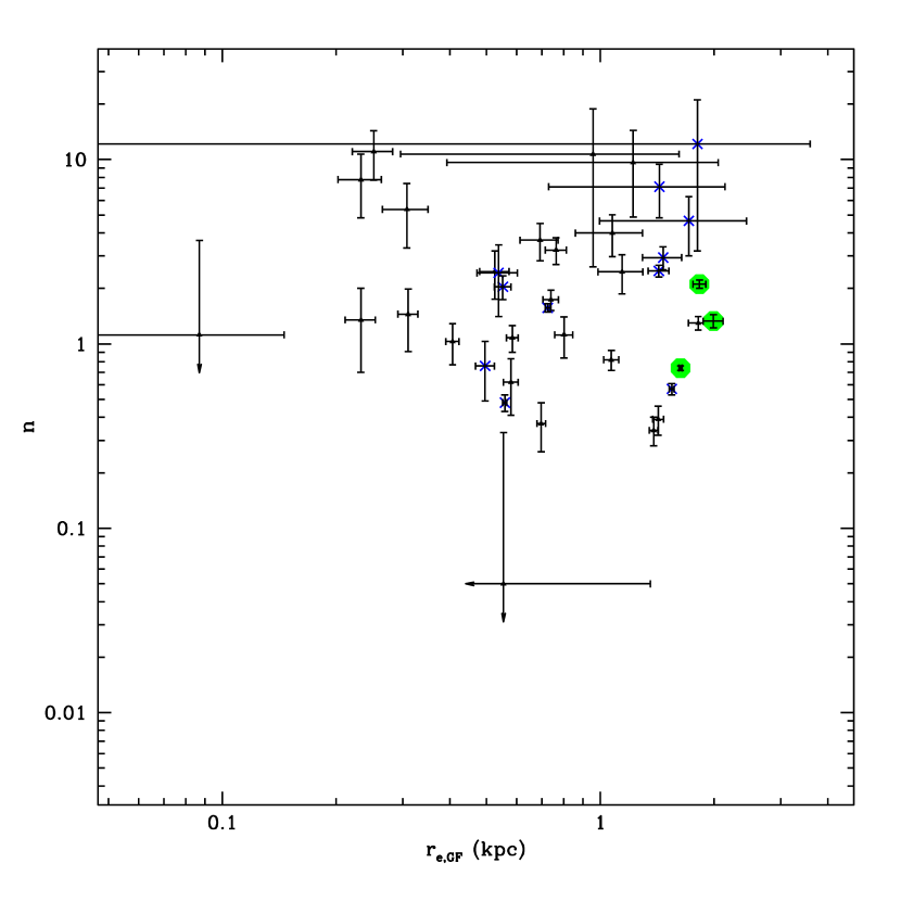
Figure 3: The best-fit half-light radii and Sérsic indices for our sample of resolved LAE components with $S/N>30$ . Black triangles are from GEMS, blue crosses are from GOODS, and green circles are from the HUDF.There is a trend seen such that components with $n\gtrsim 2$ have an excess of diffuse emission at large radii, while components with $n\lesssim 2$ have extended or multi-compent light distributions.

Table 1 gives the Sérseic indices for all our resolved LAE components with $S/N>30$. Of these 52 objects components analyzed, GALFIT converged on a solution for 48 of them, while the results for two others (both components of LAE 12) were discarded due to contamination from a bright extended source just outside the selection circle. These best-fit Sérsic indices, $n$, are plotted against the intrinsic half-light radii, $r_{e,GF}$, in Figure 3. A cursory examination of the figure reinforces the fact that most LAE components are extremely compact: although UV emission from LAEs can have a range of half-light radii from $\lesssim 0.3$ kpc (predominantly point sources, not plotted) to $\sim 2$ kpc, the majority are very small, with $r_{e,GF}<1$ kpc. This result is similar to that found for LAEs at $z=4.1$ to $5.7$ by Pirzkal et al. (2007); Overzier et al. (2008); Taniguchi et al. (2009).

A histogram of the Sérsic indices is shown in Figure 4. Although the distribution is broad, with values ranging from $n\lesssim 1$ to $n\gtrsim 12$, the majority of LAEs have small Sérsic indices, and the peak of the distribution is at $n\sim 1.5$. This is simlar to what is seen for nearby galaxies from the Sloan Digital Sky Survey (Blanton & Moustakas 2009) although our distribution lacks the high-$n$ population associated with massive, red galaxies. Moreover, a visual inspection of the images shows a morphological transition at $n\sim 2$. Components with small $n$ generally have extended or split peaks in their luminosity profile, with relatively little diffuse emission beyond $2r_{e,GF}$. While it is possible that these objects be merging systems, multiple star-forming clumps in close proximity to each other can also conspire to produce small values of $n$ (e.g., Rawat et al. 2009). By contrast, LAE components with $n\gtrsim 2$ have high concentration cores, surrounded by diffuse emission that often extends to many $r_{e,GF}$. Interestingly, unlike in low-redshift spheroids, this diffuse emission is often amorphous or clumpy. It is possible that these compact components represent bulges in the act of formation, or, alternatively, isolated star-forming regions within a larger galaxy.

4.3.1 Robustness of the Sérsic Fits

The uncertainties reported by GALFIT on the Sérsic index reported in Table 1 are based upon the local curvature of the $\chi^{2}$ surfaces, and therefore do not account of systematic errors in the analysis. In their study of LBGs within the GOODS fields, Ravindranath et al. (2006) simulated $50,000$ pure $n=1$ and $n=4$ systems with magnitudes $21<V<27$ and half-light radii ($0\farcs 01<r_{e}<5\farcs 0$). They found that for objects with magnitudes ($25<V<26.6$) and sizes ($r_{e}<0\farcs 13$) considered here, the GALFIT fitting procedure typically has a random uncertainty of $\sigma_{n}\sim 1.5$ for spheroids and $\sigma_{n}\sim 0.5$ for disks (see their Figure 4). Their simulations also demonstrate that the GALFIT algorithms have a tendency to overestimate $n$ for disk systems ($\langle n\rangle\sim 1.1$) and to underestimate $n$ in spheroids ($\langle n\rangle\sim 3.83$). Häussler et al. (2007) found similar results in their GALFIT sutdy of high-redshift galaxies in GEMS.

An alternative way of investigating the systematic tendencies of GALFIT is to perform a direct comparison of independent observations of galaxies taken to different depths. Between HUDF, GOODS, and sGOODS, there are 6 LAEs with components that are resolved in more than one survey. Table 3 lists these objects, along with the best-fit $V$-band magnitude, $V_{GF}$, half-light radii, and Sérsic index for the brightest component of each object. The table demonstrates that there is a slight tendency for high redshift LAEs to appear dimmer and smaller in shallower surveys, and for these surveys to overestimate $n$. However, since the weighted mean difference between sGOODS and GOODS, $\Delta n_{GG}=0.65\pm 0.01$, is significantly larger than that between HUDF and GOODS, $\Delta n_{HG}=0.215\pm 0.001$, the data suggest that the GOODS imaging is deep enough to allow us to distinguish point sources from more extended objects.

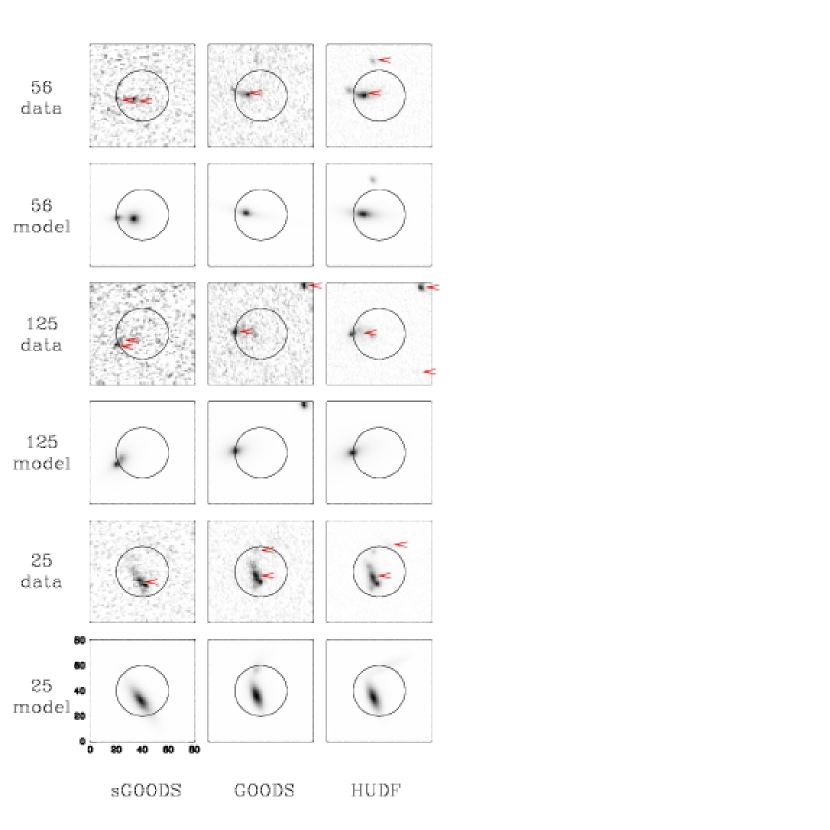
Figure 5: The images and best-fit Sérsic profiles for the three LAEs with HUDF, GOODS, and sGOODs data. We mark all possible component detections with red arrows in the data panels and draw the selection circle in black for all panels. Cutouts are $2\farcs 4\times 2\farcs 4$ on a side.

Figure 5 displays the sGOODS, GOODS, and HUDF images for the 3 LAE components in the HUDF field, and compares them to their Sérsic fits. The brightest of the three sources, LAE 25 ($V_{GF}\sim 25$), is well fit by a Sérsic disk ($n\sim 1$) with $r_{e,GF}\sim 1.5$ kpc. (Additional components are detected in the deeper surveys but have $V_{GF}>27.5$ and are indistinguishable from point sources.) In contrast, the GOODS and sGOODS fits fits for LAE $56$ and LAE $125$ (both with $V_{GF}\sim 26.5$) are highly uncertain, despite their large half-light radii ($\sim 1.8$ kpc). This is due to the asymmetric associated with the diffuse emission surrounding the objects’ central cores: any attempt to fit these irregular features with a simple model will have difficulty. In fact, in the sGOODS data, SExtractor divided the primary components of these objects in two, turning resolved LAEs into multiple discrete sources. Thus, the interpretation of LAEs 56 and 125 are not straightforward.

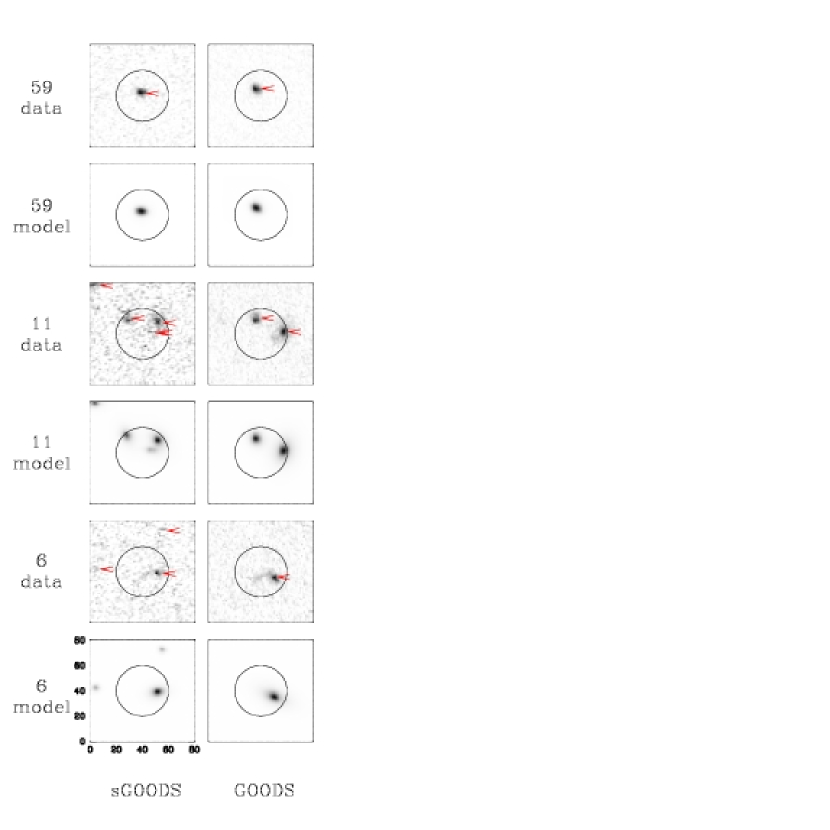
Figure 6: Same as Figure 5, but for the three resolved LAEs having only GOODS and sGOODS coverage.

Three additional sources were resolved in both GOODS and sGOODS; these are plotted in Figure 6. Of the three, LAE $6$ has the brightest single component at $V_{GF}\sim 25.4$ and fits to this source are fairly robust, with $r_{e,GF}\sim 0.6$ kpc and $n\lesssim 0.5$. LAE 11, however, has two bright components within the selection circle (only the results for the brightest component are given in Table 3) as well as some diffuse light, possibly associated with an interaction. The inconsistencies between the GOODS and sGOODS fits are primarily due to the additional (and likely spurious) detections in the sGOODS image. Finally, for LAE 59, GALFIT produced single component models for both the GOODS and the sGOODS data. However, since the latter fit failed to generate an error bar, we have removed the object from the table.

5 Discussion

From Figures 5 and 6 it is clear that our sample of $z\sim 3$ LAEs have a broad range of morphologies. While most sources are small ($r_{e}<2$ kpc) and concentrated ($2<C<4$), the rest-frame UV emission from a typical LAE is neither smooth nor symmetrical. LAE ellipticities are skewed towards higher values of $\epsilon$, in a manner similar to that seen for LBGs at the same redshift (Ravindranath et al. 2006). This suggests the presence of elongated, prolate structures, which may be indicative of merging activity or “chain” star formation. Unfortunately, it is difficult to probe the concentration indices of the population: even for the subset of LAEs that GALFIT calls resolved, the distribution of $C$ values is similar to that measured for stars. Next generation space-based imagers are needed to properly probe this parameter.

Our LAEs also possess a broad range of Sérsic indices (see Figure 4). As in the local universe (Blanton & Moustakas 2009), the distribution of $n$ values peaks near $\sim 1$ with a broad distribution with values ranging from $n\lesssim 1$ and $n\gtrsim 12$. Our population does not, however, have the high-$n$ population associated with luminous, red galaxies in the local universe. Whether we are observing the formation of the Hubble sequence is not clear, but there does appear to be a qualitative change in morphology at $n\sim 2$. At greater $n$ values, LAE components appear more compact, relative to their surrounding diffuse emission, than objects with $n\sim 1$. However, these “spheroid-like” LAEs could also be the result of compact star-forming regions imbedded in the diffuse emission of a disk-like or irregular galaxy. Deeper imaging is required to make this distinction.

If we classify LAEs with $n>2.5$ as “bulge-like” and LAEs with $2.5\geq n>0.8$ as ”disk-like” we find that 31% of our sample of resolved LAE components with $S/N>30$ fall into the former category, while 44% belong to the latter. In a sample of LBGs at the same redshift, Ravindranath et al. (2006) found 27% were bulge-like and 42% were disk-like. From the data, it appears that the light profiles of LBGs and LAEs at this redshift have similar distributions.

A subset of our LAEs consist of multiple components, and this can be interpreted as evidence for merger activity. When interacting systems are in close proximity, they may appear as as one single object with a small value of $n$ (see, for example, LAE $25$ in Figure 5). If we follow Ravindranath et al. (2006) and consider sources with $n<0.8$ (i.e., with light profiles that are flatter than exponential) to be merger candidates, then $\sim 24$% of our sample would be classified as such. This again is consistent with the 31% value found by Ravindranath et al. (2006) for LBGs at a similar redshift. We note that in a stacked sample of $z\sim 5.7$ LAEs created by Taniguchi et al. (2009), $n\sim 0.7$ which may indicate a larger fraction of merger candidates in LAE samples at higher redshift. The sample of Taniguchi, however, covers a significantly brighter range of Ly$\alpha$ luminosity ( $3\times 10^{43}$ to $6.3\times 10^{42}$ ergs sec^-1) than our sample at $z\sim 3.1$ ($\sim 10^{43}$ to $1.3\times 10^{42}$ ergs sec^-1). Ideally, such a comparison between morphological properties of LAE samples would be done by comparing samples at similar luminosities, but such samples do not currently exist besides that presented here.

Of course, estimating merger rate using measured $n$ values fails to account for LAEs in which the interacting galaxies are at large separation. In these cases, SExtractor will consider the objects separate as components (see, for example, LAE $11$ in Figure 6). On the other hand, galaxies with clumpy internal star formation can be mistaken for mergers when viewed in the rest-frame UV. Clumpy star-formation will lead also to low measured values of $n$ (e.g., Rawat et al. 2009) and hence an overestimate of the estimated merger rate. To rule out this possibility, and to make progress towards determining the true LAE merger fraction, we would require deep $V$-band imaging ($m_{lim,5\sigma}\sim 30$) for a much larger sample of LAEs than is covered by the HUDF.

Our morphological results for LAEs at $z\sim 3$ are broadly similar to those found for continuum-selected LBG objects at the same redshift. This consistency supports the contention of Law et al. (2007) and Pentericci et al. (2010) that that the presence of Ly$\alpha$ in emission has little bearing on rest-frame UV morphology of $z\sim 3$ star-forming galaxies. Comparable results were also found by Taniguchi et al. (2009) at $z\sim 6$, and may support a scenario in which the observed differences between LAEs and LBGs are driven by variations in dust content and HI gas (Verhamme et al. 2008). On the other hand Vanzella et al. (2009) found that dropout galaxies at $z\sim 4$ with Ly$\alpha$-emission were significantly more concentrated than the rest of the sample. Disentangling the effects of emission-line strength on morphology as a function of redshift will require substantially larger samples with deep high-resolution imaging at multiple redshifts, preferably tracking the same rest-frame continuum wavelength free of contamination from the Ly$\alpha$ emission line.

Our results for the morphologies of $z\sim 3$ LAEs highlight the need for consistency between measurements made at different survey depths and the need for systematic checks to verify the robustness of derived parameters. It also points out the importance of making measurements consistently over a wide range of redshifts. This paper represents the first attempt to measure morphological parameters of a large sample of LAEs as previous work has concentrated primarily on measuring sizes (Venemans et al. 2005; Bond et al. 2009), used small ($n\lesssim 12$) sample sizes (Overzier et al. 2008; Pirzkal et al. 2007), or measured the profiles of a stacked sample due to low signal-to-noise (Taniguchi et al. 2009). The advent of larger samples of LAEs from redshifts ranging from $z=2.1$ to $z>7$ should allow for meaningful comparisons across redshifts down to similar luminosity limits to be made. Without such data, it is impossible to form a clear picture of how the process of galaxy formation proceeds over time.

The measurements presented here are limited by the fact that we are observing the morphologies of these high-redshift galaxies in the rest-frame ultraviolet where individual clumps of on-going star-formation may strongly affect the light distributions (e.g., Overzier et al. 2010). Future work in the rest-frame optical (observed infrared) using WFC3 on HST should alleviate some of these concerns, and allow us the bulk of the LAE stellar population. A comparison of the two bandpasses will then enable us to examine how star formation proceeds in these objects.

6 Acknowledgements

Support for this work was provided by NASA through grants HST-AR-10324.01-A & HST-AR-11253.01-A from the Space Telescope Science Institute, which is operated by AURA, Inc., under NASA contract NAS 5-26555 and by the National Science Foundation under grants AST-0807885 & AST-0807570. We thank Justin McKane for his assistance with the analysis. Some of the data presented in this paper were obtained from the Multimission Archive at the Space Telescope Science Institute (MAST). STScI is operated by the Association of Universities for Research in Astronomy, Inc., under NASA contract NAS5-26555. Support for MAST for non-HST data is provided by the NASA Office of Space Science via grant NAG5-7584 and by other grants and contracts.

Table 1: LAE Component Morphological Properties

Object	Component	Survey	$\alpha$	$\delta$	$V_{GF}$	$r_{e,GF}$	$n$	$b/a$	$C$
						(kpc)
$25$	$1$	HUDF	$3$:$32$:$40.779$	$-27$:$46$:$06.076$	$25.11\pm 0.01$	$1.63\pm 0.01$	$0.74\pm 0.02$	$0.29\pm 0.00$	$2.60$
$56$	$1$	HUDF	$3$:$32$:$34.324$	$-27$:$47$:$59.559$	$26.24\pm 0.02$	$1.83\pm 0.07$	$2.11\pm 0.11$	$0.25\pm 0.01$	$3.01$
$125$	$1$	HUDF	$3$:$32$:$39.017$	$-27$:$46$:$22.287$	$26.47\pm 0.04$	$1.99\pm 0.12$	$1.33\pm 0.11$	$0.40\pm 0.02$	$2.07$
$4$	$1$	GOODS	$3$:$32$:$18.817$	$-27$:$42$:$48.190$	$25.25\pm 0.02$	$0.73\pm 0.01$	$1.57\pm 0.08$	$0.51\pm 0.02$	$2.55$
	$2$	GOODS	$3$:$32$:$18.791$	$-27$:$42$:$48.215$	$27.42\pm 0.32$	$0.30\pm 0.15$	$7.97\pm 11.08$	$0.35\pm 0.22$
	$3$	GOODS	$3$:$32$:$18.840$	$-27$:$42$:$47.789$	$27.60\pm 0.33$	$0.88\pm 0.44$	$2.52\pm 2.10$	$0.60\pm 0.16$
	$4$	GOODS	$3$:$32$:$18.800$	$-27$:$42$:$47.863$	$27.62\pm 0.11$	$1.19\pm 0.19$	$1.08\pm 0.50$	$0.14\pm 0.07$
$6$	$1$	GOODS	$3$:$32$:$52.689$	$-27$:$48$:$09.264$	$25.37\pm 0.01$	$0.56\pm 0.01$	$0.48\pm 0.05$	$0.48\pm 0.01$	$2.32$
$11$	$1$	GOODS	$3$:$32$:$26.925$	$-27$:$41$:$28.010$	$25.41\pm 0.04$	$1.43\pm 0.09$	$2.49\pm 0.18$	$0.68\pm 0.02$	$2.85$
	$2$	GOODS	$3$:$32$:$26.968$	$-27$:$41$:$27.723$	$26.25\pm 0.03$	$0.55\pm 0.03$	$2.04\pm 0.30$	$0.77\pm 0.05$	$2.33$
$25$	$1$	GOODS	$3$:$32$:$40.783$	$-27$:$46$:$06.057$	$25.19\pm 0.01$	$1.55\pm 0.02$	$0.57\pm 0.04$	$0.30\pm 0.01$	$2.57$
$35$	$1$	GOODS	$3$:$32$:$45.603$	$-27$:$52$:$10.897$	$27.02\pm 0.03$	$0.41\pm 0.03$	$1.29\pm 0.46$	$0.55\pm 0.07$	$2.52$
$41$	$1$	GOODS	$3$:$32$:$56.671$	$-27$:$49$:$49.174$	$26.63\pm 0.05$	$0.54\pm 0.07$	$2.43\pm 1.02$	$0.18\pm 0.10$	$2.67$
$44$	$1$	GOODS	$3$:$32$:$15.790$	$-27$:$44$:$09.902$	$26.23\pm 0.22$	$1.43\pm 0.70$	$7.12\pm 2.29$	$0.60\pm 0.07$	$3.37$
	$2$	GOODS	$3$:$32$:$15.809$	$-27$:$44$:$10.069$	$26.91\pm 0.09$	$1.43\pm 0.15$	$1.11\pm 0.19$	$0.51\pm 0.04$	$2.25$
$56$	$1$	GOODS	$3$:$32$:$34.327$	$-27$:$47$:$59.549$	$26.50\pm 0.37$	$1.81\pm 1.78$	$12.16\pm 8.96$	$0.10\pm 0.05$	$2.71$
$59$	$1$	GOODS	$3$:$32$:$33.250$	$-27$:$51$:$27.576$	$25.80\pm 0.07$	$1.47\pm 0.17$	$2.94\pm 0.42$	$0.43\pm 0.03$	$3.19$
$94$	$1$	GOODS	$3$:$32$:$09.335$	$-27$:$43$:$54.177$	$26.64\pm 0.02$	$0.50\pm 0.03$	$0.76\pm 0.27$	$0.59\pm 0.05$	$2.54$
$125$	$1$	GOODS	$3$:$32$:$39.007$	$-27$:$46$:$22.268$	$26.40\pm 0.21$	$1.72\pm 0.72$	$4.65\pm 1.65$	$0.51\pm 0.08$
$8$	$1$	GEMS	$3$:$31$:$54.883$	$-27$:$51$:$21.104$	$25.44\pm 0.01$	$0.55\pm 0.80$	$0.05\pm 0.28$	$0.39\pm 0.03$	$2.44$
$9$	$1$	GEMS	$3$:$31$:$40.150$	$-28$:$03$:$07.395$	$25.17\pm 0.01$	$0.09\pm 0.06$	$1.12\pm 2.52$	$0.67\pm 0.18$	$2.58$
$10$	$1$	GEMS	$3$:$33$:$22.453$	$-27$:$46$:$36.909$	$25.81\pm 0.01$	$0.41\pm 0.02$	$1.03\pm 0.26$	$0.22\pm 0.04$
$13$	$1$	GEMS	$3$:$33$:$07.252$	$-27$:$47$:$47.188$	$25.58\pm 0.04$	$0.76\pm 0.05$	$3.23\pm 0.53$	$0.31\pm 0.03$	$2.77$
$15$	$1$	GEMS	$3$:$33$:$18.920$	$-27$:$38$:$28.462$	$26.53\pm 0.03$	$0.99\pm 2.73$	$0.03\pm 0.37$	$0.34\pm 0.04$	$2.14$
$17$	$1$	GEMS	$3$:$32$:$49.147$	$-27$:$34$:$39.932$	$25.59\pm 0.03$	$0.74\pm 0.04$	$1.74\pm 0.22$	$0.78\pm 0.04$	$2.76$
$18$	$1$	GEMS	$3$:$32$:$46.753$	$-27$:$39$:$59.909$	$26.68\pm 0.03$	$0.30\pm 0.03$	$1.39\pm 0.73$	$0.73\pm 0.12$	$2.35$
$19$	$1$	GEMS	$3$:$31$:$34.736$	$-27$:$56$:$21.803$	$25.03\pm 0.09$	$0.25\pm 0.03$	$11.06\pm 3.31$	$0.81\pm 0.07$	$2.91$
$20$	$1$	GEMS	$3$:$33$:$11.882$	$-28$:$00$:$12.561$	$26.40\pm 0.07$	$1.06\pm 0.10$	$1.01\pm 0.17$	$0.91\pm 0.07$	$2.75$
	$2$	GEMS	$3$:$33$:$11.871$	$-28$:$00$:$12.121$	$26.58\pm 0.03$	$0.57\pm 0.03$	$0.90\pm 0.35$	$0.55\pm 0.06$	$2.53$
$22$	$1$	GEMS	$3$:$31$:$51.634$	$-27$:$58$:$32.617$	$26.26\pm 0.04$	$0.31\pm 0.04$	$5.37\pm 2.05$	$0.16\pm 0.08$	$2.83$
$24$	$1$	GEMS	$3$:$31$:$53.212$	$-27$:$57$:$08.156$	$26.24\pm 0.02$	$0.23\pm 0.02$	$1.35\pm 0.65$	$0.46\pm 0.10$	$2.61$
$26$	$1$	GEMS	$3$:$31$:$51.560$	$-27$:$46$:$47.005$	$26.39\pm 0.03$	$1.02\pm 0.04$	$0.20\pm 0.10$	$0.58\pm 0.03$	$2.05$
$29$	$1$	GEMS	$3$:$31$:$47.795$	$-27$:$45$:$03.300$	$26.65\pm 0.05$	$0.41\pm 0.09$	$3.52\pm 1.27$	$0.37\pm 0.11$	$1.20$
$36$	$1$	GEMS	$3$:$32$:$18.925$	$-27$:$38$:$40.183$	$26.94\pm 0.10$	$0.65\pm 0.10$	$2.50\pm 1.26$	$0.48\pm 0.11$	$3.53$
$38$	$1$	GEMS	$3$:$31$:$50.358$	$-27$:$59$:$10.099$	$26.42\pm 0.02$	$0.56\pm 2.04$	$0.04\pm 0.35$	$0.26\pm 0.08$	$2.25$
$39$	$1$	GEMS	$3$:$31$:$30.522$	$-27$:$47$:$29.637$	$25.33\pm 0.04$	$1.82\pm 0.10$	$1.30\pm 0.11$	$0.39\pm 0.02$	$2.84$
$43$	$1$	GEMS	$3$:$33$:$07.314$	$-27$:$54$:$38.985$	$25.69\pm 0.10$	$0.23\pm 0.03$	$7.78\pm 2.95$	$0.97\pm 0.10$	$2.70$
$49$	$1$	GEMS	$3$:$31$:$42.357$	$-27$:$58$:$07.834$	$25.79\pm 0.02$	$1.38\pm 0.04$	$0.34\pm 0.06$	$0.38\pm 0.01$	$2.34$
$50$	$1$	GEMS	$3$:$31$:$52.829$	$-27$:$45$:$18.631$	$26.90\pm 0.15$	$0.76\pm 0.05$	$0.11\pm 0.32$	$0.12\pm 0.12$	$2.16$
$53$	$1$	GEMS	$3$:$32$:$15.130$	$-27$:$38$:$53.937$	$25.82\pm 0.02$	$1.42\pm 0.05$	$0.39\pm 0.07$	$0.48\pm 0.02$	$2.24$
$61$	$1$	GEMS	$3$:$33$:$09.435$	$-27$:$45$:$50.102$	$26.41\pm 0.13$	$1.07\pm 0.23$	$2.46\pm 0.86$	$0.47\pm 0.08$	$2.15$
$63$	$1$	GEMS	$3$:$32$:$51.916$	$-27$:$42$:$12.234$	$25.75\pm 0.02$	$0.59\pm 0.02$	$1.08\pm 0.18$	$0.54\pm 0.03$	$2.63$
$64$	$1$	GEMS	$3$:$31$:$59.830$	$-27$:$49$:$46.413$	$25.80\pm 0.27$	$1.22\pm 0.83$	$9.65\pm 4.76$	$0.70\pm 0.11$	$2.58$
$67$	$1$	GEMS	$3$:$32$:$51.768$	$-27$:$37$:$33.540$	$26.27\pm 0.02$	$0.31\pm 0.02$	$1.45\pm 0.54$	$0.42\pm 0.06$	$2.06$
$69$	$1$	GEMS	$3$:$33$:$25.356$	$-28$:$02$:$46.519$	$25.99\pm 0.03$	$1.07\pm 0.05$	$0.82\pm 0.10$	$0.53\pm 0.03$	$3.42$
$73$	$1$	GEMS	$3$:$32$:$57.403$	$-27$:$55$:$19.055$	$26.57\pm 0.03$	$0.31\pm 0.03$	$1.91\pm 0.63$	$0.70\pm 0.09$	$3.72$
$75$	$1$	GEMS	$3$:$32$:$59.267$	$-27$:$41$:$14.734$	$27.01\pm 0.04$	$0.49\pm 0.04$	$0.66\pm 0.53$	$0.10\pm 0.17$	$2.50$
$82$	$1$	GEMS	$3$:$31$:$47.775$	$-27$:$42$:$16.311$	$26.32\pm 0.02$	$0.58\pm 0.03$	$0.62\pm 0.21$	$0.55\pm 0.04$	$2.37$
$83$	$1$	GEMS	$3$:$31$:$38.669$	$-27$:$45$:$43.551$	$26.48\pm 0.08$	$0.85\pm 0.10$	$1.87\pm 0.61$	$0.49\pm 0.07$	$2.45$
$87$	$1$	GEMS	$3$:$33$:$05.025$	$-27$:$43$:$37.295$	$25.97\pm 0.10$	$1.08\pm 0.22$	$4.00\pm 1.03$	$0.49\pm 0.06$	$3.55$
$91$	$1$	GEMS	$3$:$31$:$58.802$	$-27$:$49$:$28.753$	$26.74\pm 0.04$	$0.88\pm 4.64$	$0.01\pm 1.12$	$0.38\pm 0.07$	$2.43$
$98$	$1$	GEMS	$3$:$31$:$26.618$	$-27$:$44$:$02.175$	$26.75\pm 0.04$	$1.04\pm 0.08$	$0.64\pm 0.21$	$0.53\pm 0.05$	$2.18$
$99$	$1$	GEMS	$3$:$31$:$40.245$	$-27$:$45$:$26.702$	$26.03\pm 0.01$	$0.70\pm 0.02$	$0.37\pm 0.11$	$0.41\pm 0.03$	$2.82$
$101$	$1$	GEMS	$3$:$33$:$07.747$	$-27$:$38$:$19.332$	$26.34\pm 0.30$	$0.96\pm 0.66$	$10.71\pm 8.09$	$0.22\pm 0.08$	$2.58$
$105$	$1$	GEMS	$3$:$33$:$12.401$	$-27$:$45$:$24.291$	$26.28\pm 0.05$	$0.53\pm 0.05$	$2.47\pm 0.72$	$0.53\pm 0.07$	$3.13$
$106$	$1$	GEMS	$3$:$32$:$21.284$	$-27$:$36$:$21.398$	$25.80\pm 0.06$	$0.69\pm 0.08$	$3.66\pm 0.84$	$0.71\pm 0.06$	$3.59$
$112$	$1$	GEMS	$3$:$32$:$43.954$	$-27$:$37$:$16.846$	$26.24\pm 0.08$	$1.14\pm 0.16$	$2.46\pm 0.59$	$0.32\pm 0.05$	$2.35$
$121$	$1$	GEMS	$3$:$33$:$23.709$	$-27$:$44$:$09.126$	$27.04\pm 0.00$	$0.50\pm 0.00$	$0.61\pm 0.00$	$0.44\pm 0.00$	$2.30$
$122$	$1$	GEMS	$3$:$32$:$20.467$	$-27$:$35$:$01.616$	$26.45\pm 0.07$	$0.46\pm 0.06$	$3.61\pm 1.42$	$0.45\pm 0.08$	$3.04$
$124$	$1$	GEMS	$3$:$31$:$42.924$	$-28$:$03$:$07.835$	$26.31\pm 0.03$	$0.80\pm 0.04$	$1.12\pm 0.28$	$0.25\pm 0.04$	$2.86$
$133$	$1$	GEMS	$3$:$31$:$42.951$	$-27$:$45$:$06.568$	$26.97\pm 0.45$	$1.74\pm 2.04$	$9.22\pm 8.60$	$0.10\pm 0.08$	$2.53$
$149$	$1$	GEMS	$3$:$33$:$07.026$	$-27$:$37$:$53.498$	$26.37\pm 0.17$	$1.43\pm 0.49$	$4.44\pm 1.71$	$0.30\pm 0.06$	$2.67$
$156$	$1$	GEMS	$3$:$33$:$00.602$	$-28$:$00$:$06.503$	$26.88\pm 0.05$	$0.80\pm 0.06$	$0.98\pm 0.37$	$0.36\pm 0.07$	$2.59$
$162$	$1$	GEMS	$3$:$33$:$15.186$	$-27$:$54$:$01.859$	$26.82\pm 0.03$	$0.64\pm 0.03$	$0.08\pm 0.36$	$0.48\pm 0.04$

Table 2: LAE System Morphological Properties

				$V^{\rm PHOT}$	$r_{e}^{\rm PHOT}$
Number	Survey	$\alpha$	$\delta$	(AB mags)	(kpc)	$b/a$	$C$
25	HUDF	$3$:$32$:$40.785$	$-27$:$46$:$06.035$	$25.04\pm 0.01$	1.48	0.57	2.60
56	HUDF	$3$:$32$:$34.329$	$-27$:$47$:$59.543$	$26.30\pm 0.02$	1.39	0.55	3.01
125	HUDF	$3$:$32$:$39.012$	$-27$:$46$:$22.307$	$26.47\pm 0.02$	1.68	0.67	2.07
4	GOODS	$3$:$32$:$18.813$	$-27$:$42$:$48.103$	$24.89\pm 0.03$	1.49	0.80	3.14
6	GOODS	$3$:$32$:$52.690$	$-27$:$48$:$09.288$	$25.38\pm 0.03$	0.71	0.86	2.32
11	GOODS	$3$:$32$:$26.938$	$-27$:$41$:$27.935$	$25.16\pm 0.03$	2.56	0.41	…
25	GOODS	$3$:$32$:$40.785$	$-27$:$46$:$05.999$	$25.04\pm 0.03$	1.52	0.54	2.51
35	GOODS	$3$:$32$:$45.604$	$-27$:$52$:$10.913$	$26.81\pm 0.11$	0.82	0.89	2.52
41	GOODS	$3$:$32$:$56.672$	$-27$:$49$:$49.202$	$26.78\pm 0.20$	0.68	0.58	2.67
44	GOODS	$3$:$32$:$15.799$	$-27$:$44$:$09.992$	$26.01\pm 0.05$	1.56	0.61	1.97
55	GOODS	$3$:$32$:$59.976$	$-27$:$50$:$26.308$	$26.37\pm 0.18$	1.28	0.47	2.29
56	GOODS	$3$:$32$:$34.331$	$-27$:$47$:$59.550$	$26.44\pm 0.11$	1.46	0.54	2.71
59	GOODS	$3$:$32$:$33.254$	$-27$:$51$:$27.590$	$25.86\pm 0.06$	1.33	0.68	3.19
66	GOODS	$3$:$32$:$48.528$	$-27$:$56$:$05.374$	$26.66\pm 0.20$	1.93	0.73	3.16
85	GOODS	$3$:$32$:$59.824$	$-27$:$53$:$05.766$	$26.62\pm 0.13$	0.74	0.90	2.54
90	GOODS	$3$:$32$:$14.574$	$-27$:$45$:$52.420$	$26.90\pm 0.16$	0.95	0.71	3.14
94	GOODS	$3$:$32$:$09.336$	$-27$:$43$:$54.192$	$26.63\pm 0.13$	0.72	0.92	2.53
125	GOODS	$3$:$32$:$39.016$	$-27$:$46$:$22.307$	$26.32\pm 0.09$	1.58	0.75	…
5	GEMS	$3$:$32$:$47.517$	$-27$:$58$:$07.705$	$24.95\pm 0.03$	1.14	0.52	2.34
8	GEMS	$3$:$31$:$54.885$	$-27$:$51$:$21.114$	$25.32\pm 0.04$	0.73	0.88	2.50
9	GEMS	$3$:$31$:$40.157$	$-28$:$03$:$07.405$	$25.06\pm 0.03$	0.58	0.93	2.58
10	GEMS	$3$:$33$:$22.442$	$-27$:$46$:$36.851$	$25.12\pm 0.04$	2.17	0.53	…
12	GEMS	$3$:$32$:$33.846$	$-27$:$36$:$35.118$	$25.26\pm 0.04$	2.30	0.59	…
13	GEMS	$3$:$33$:$07.253$	$-27$:$47$:$47.177$	$25.72\pm 0.07$	0.82	0.78	2.77
15	GEMS	$3$:$33$:$18.916$	$-27$:$38$:$28.468$	$25.75\pm 0.07$	1.99	0.44	…
17	GEMS	$3$:$32$:$49.148$	$-27$:$34$:$39.972$	$25.55\pm 0.06$	1.03	0.84	2.76
18	GEMS	$3$:$32$:$46.753$	$-27$:$39$:$59.915$	$26.72\pm 0.16$	0.63	0.93	2.35
19	GEMS	$3$:$31$:$34.738$	$-27$:$56$:$21.818$	$25.08\pm 0.04$	0.81	0.90	2.91
20	GEMS	$3$:$33$:$11.879$	$-28$:$00$:$12.380$	$25.82\pm 0.07$	1.93	0.42	…
22	GEMS	$3$:$31$:$51.636$	$-27$:$58$:$32.646$	$26.18\pm 0.10$	0.78	0.74	2.83
24	GEMS	$3$:$31$:$53.213$	$-27$:$57$:$08.161$	$26.18\pm 0.09$	0.61	0.88	2.61
26	GEMS	$3$:$31$:$51.562$	$-27$:$46$:$47.014$	$26.16\pm 0.10$	1.17	0.79	2.05
29	GEMS	$3$:$31$:$47.801$	$-27$:$45$:$03.384$	$26.35\pm 0.12$	1.23	0.67	2.89
36	GEMS	$3$:$32$:$18.926$	$-27$:$38$:$40.196$	$26.99\pm 0.21$	0.81	0.72	3.53
38	GEMS	$3$:$31$:$50.370$	$-27$:$59$:$10.122$	$26.52\pm 0.13$	0.60	0.87	2.25
39	GEMS	$3$:$31$:$30.524$	$-27$:$47$:$29.648$	$25.33\pm 0.04$	1.58	0.74	2.84
41	GEMS	$3$:$32$:$56.672$	$-27$:$49$:$49.242$	$26.55\pm 0.14$	0.94	0.75	3.07
43	GEMS	$3$:$33$:$07.315$	$-27$:$54$:$38.988$	$25.78\pm 0.07$	0.74	0.90	2.70
49	GEMS	$3$:$31$:$42.359$	$-27$:$58$:$07.856$	$25.69\pm 0.06$	1.26	0.66	2.34
52	GEMS	$3$:$33$:$21.363$	$-27$:$38$:$36.337$	$26.91\pm 0.19$	0.55	0.87	2.69
53	GEMS	$3$:$32$:$15.131$	$-27$:$38$:$53.948$	$25.82\pm 0.07$	1.25	0.79	…
55	GEMS	$3$:$32$:$59.982$	$-27$:$50$:$26.369$	$26.37\pm 0.12$	1.64	0.75	2.50
58	GEMS	$3$:$33$:$06.943$	$-27$:$42$:$27.853$	$26.61\pm 0.14$	1.03	0.79	3.59
61	GEMS	$3$:$33$:$09.422$	$-27$:$45$:$50.112$	$26.08\pm 0.07$	1.79	0.90	…
63	GEMS	$3$:$32$:$51.918$	$-27$:$42$:$12.247$	$25.66\pm 0.06$	0.81	0.85	2.63
64	GEMS	$3$:$31$:$59.831$	$-27$:$49$:$46.427$	$25.99\pm 0.08$	1.13	0.92	2.57
67	GEMS	$3$:$32$:$51.769$	$-27$:$37$:$33.550$	$26.45\pm 0.12$	0.55	0.88	2.44
68	GEMS	$3$:$32$:$58.140$	$-27$:$48$:$04.878$	$26.70\pm 0.16$	1.34	0.28	2.17
69	GEMS	$3$:$33$:$25.356$	$-28$:$02$:$46.532$	$26.12\pm 0.09$	0.99	0.76	2.54
73	GEMS	$3$:$32$:$57.404$	$-27$:$55$:$19.074$	$26.31\pm 0.11$	0.85	0.83	3.78
74	GEMS	$3$:$33$:$18.588$	$-27$:$45$:$42.620$	$26.67\pm 0.13$	0.74	0.89	2.40
75	GEMS	$3$:$32$:$59.268$	$-27$:$41$:$14.752$	$26.87\pm 0.19$	0.77	0.69	2.50
79	GEMS	$3$:$31$:$58.027$	$-27$:$47$:$30.332$	$26.26\pm 0.09$	1.70	0.43	2.92
82	GEMS	$3$:$31$:$47.776$	$-27$:$42$:$16.326$	$26.43\pm 0.12$	0.67	0.87	2.38
83	GEMS	$3$:$31$:$38.670$	$-27$:$45$:$43.589$	$26.52\pm 0.11$	0.96	0.73	2.52
87	GEMS	$3$:$33$:$05.026$	$-27$:$43$:$37.308$	$25.98\pm 0.08$	1.26	0.80	3.55
89	GEMS	$3$:$33$:$12.016$	$-27$:$58$:$39.929$	$26.66\pm 0.16$	1.38	0.12	2.91
91	GEMS	$3$:$31$:$58.803$	$-27$:$49$:$28.765$	$26.91\pm 0.19$	0.63	0.78	2.43
92	GEMS	$3$:$33$:$03.319$	$-27$:$41$:$39.041$	$26.98\pm 0.21$	2.32	0.41	…
98	GEMS	$3$:$31$:$26.621$	$-27$:$44$:$02.177$	$26.55\pm 0.14$	1.24	0.73	2.12
99	GEMS	$3$:$31$:$40.241$	$-27$:$45$:$26.827$	$25.78\pm 0.07$	1.43	0.91	1.98
101	GEMS	$3$:$33$:$07.750$	$-27$:$38$:$19.356$	$26.61\pm 0.15$	0.86	0.52	2.58
105	GEMS	$3$:$33$:$12.403$	$-27$:$45$:$24.307$	$26.28\pm 0.11$	0.81	0.88	3.13
106	GEMS	$3$:$32$:$21.285$	$-27$:$36$:$21.341$	$25.62\pm 0.06$	1.31	0.81	3.09
112	GEMS	$3$:$32$:$44.073$	$-27$:$37$:$17.810$	$26.41\pm 0.12$	0.96	0.59	2.35
113	GEMS	$3$:$31$:$35.944$	$-27$:$50$:$52.915$	$26.57\pm 0.14$	1.75	0.79	3.20
121	GEMS	$3$:$33$:$23.709$	$-27$:$44$:$09.139$	$26.97\pm 0.21$	0.71	0.82	2.30
122	GEMS	$3$:$32$:$20.465$	$-27$:$35$:$01.630$	$26.48\pm 0.13$	0.75	0.98	3.03
124	GEMS	$3$:$31$:$42.925$	$-28$:$03$:$07.798$	$26.01\pm 0.08$	1.22	0.64	…
126	GEMS	$3$:$31$:$44.374$	$-27$:$50$:$57.700$	$26.29\pm 0.11$	0.91	0.91	3.67
127	GEMS	$3$:$33$:$02.820$	$-27$:$57$:$17.507$	$26.94\pm 0.20$	0.74	0.86	2.64
149	GEMS	$3$:$33$:$07.027$	$-27$:$37$:$53.512$	$26.37\pm 0.12$	1.27	0.64	2.67
152	GEMS	$3$:$33$:$29.304$	$-27$:$36$:$41.785$	$25.93\pm 0.08$	2.25	0.67	2.51
156	GEMS	$3$:$33$:$00.604$	$-28$:$00$:$06.538$	$26.88\pm 0.18$	0.85	0.73	2.59
157	GEMS	$3$:$33$:$28.389$	$-27$:$45$:$09.634$	$26.84\pm 0.19$	1.71	0.72	2.28
162	GEMS	$3$:$33$:$15.184$	$-27$:$54$:$01.638$	$25.74\pm 0.07$	2.31	0.54	…

Table 3: Morphological Properties vs. Depth for LAEs with Multiple Coverage

Number	$V_{GF}$			$r_{e,GF}$			$n$
	HUDF	GOODS	sGOODS	HUDF	GOODS	sGOODS	HUDF	GOODS	sGOODS
	(AB mags)	(AB mags)	(AB mags)	(kpc)	(kpc)	(kpc)
GLAE$6$	$--$	$25.37\pm 0.01$	$25.39\pm 0.07$	$--$	$0.56\pm 0.01$	$0.58\pm 0.02$	$--$	$0.48\pm 0.05$	$0.10\pm 0.14$
GLAE$11$	$--$	$25.41\pm 0.04$	$25.94\pm 0.20$	$--$	$1.43\pm 0.09$	$0.94\pm 0.31$	$--$	$2.49\pm 0.18$	$4.22\pm 1.47$
GLAE$25$	$25.11\pm 0.01$	$25.19\pm 0.01$	$24.92\pm 0.03$	$1.63\pm 0.01$	$1.55\pm 0.02$	$2.01\pm 0.10$	$0.74\pm 0.02$	$0.57\pm 0.04$	$1.13\pm 0.09$
GLAE$56$	$26.24\pm 0.02$	$26.50\pm 0.37$	$26.68\pm 0.15$	$1.83\pm 0.07$	$1.81\pm 1.78$	$0.71\pm 0.15$	$2.11\pm 0.11$	$12.16\pm 8.96$	$1.85\pm 1.09$
GLAE$125$	$26.47\pm 0.04$	$26.40\pm 0.21$	$26.90\pm 0.67$	$1.99\pm 0.12$	$1.71\pm 0.72$	$1.74\pm 1.79$	$1.33\pm 0.11$	$4.65\pm 1.65$	$3.22\pm 2.66$

Figure 1: Distribution of concentration (C) indices for our sample of resolved LAE components (solid line), systems (dashed line), and for a subsample of stars from the GEMS images (dotted line).

Figure 2: Top panel: Distribution of ellipticities ($1-b/a$) for our sample of resolved LAE components with $S/N>30$ (shaded histogram) and for stars on the GEMS images (solid black line). Bottom panel: Distribution of ellipticities for our sample of LAE systems with $S/N>30$.

Figure 4: Distribution of Sérsic indices for our sample of resolved LAE components with $S/N>30$. There is a broad distribution in $n$ with a peak at $n\sim 1$.

References

- Altmann et al. (2006) Altmann, M., Méndez, R. A., van Altena, W., Korchargin, V., & Ruiz, M. T. 2006, in Revista Mexicana de Astronomia y Astrofisica Conference Series, Vol. 26, Revista Mexicana de Astronomia y Astrofisica Conference Series, 64–65
- Beckwith et al. (2006) Beckwith, S. V. W. et al. 2006, AJ, 132, 1729
- Benson et al. (2007) Benson, A. J., Džanović, D., Frenk, C. S., & Sharples, R. 2007, MNRAS, 379, 841
- Benson et al. (2002) Benson, A. J., Frenk, C. S., & Sharples, R. M. 2002, ApJ, 574, 104
- Bertin & Arnouts (1996) Bertin, E. & Arnouts, S. 1996, A&AS, 117, 393
- Blanton & Moustakas (2009) Blanton, M. R. & Moustakas, J. 2009, ARA&A, 47, 159
- Bond et al. (2009) Bond, N. A., Gawiser, E., Gronwall, C., Ciardullo, R., Altmann, M., & Schawinski, K. 2009, ApJ, 705, 639
- Casertano et al. (2000) Casertano, S., de Mello, D., Dickinson, M., Ferguson, H. C., Fruchter, A. S., Gonzalez-Lopezlira, R. A., Heyer, I., Hook, R. N., Levay, Z., Lucas, R. A., Mack, J., Makidon, R. B., Mutchler, M., Smith, T. E., Stiavelli, M., Wiggs, M. S., & Williams, R. E. 2000, AJ, 120, 2747
- Conselice (2003) Conselice, C. J. 2003, ApJS, 147, 1
- Conselice et al. (2005) Conselice, C. J., Blackburne, J. A., & Papovich, C. 2005, ApJ, 620, 564
- Conselice et al. (2004) Conselice, C. J. et al. 2004, ApJ, 600, L139
- Cowie & Hu (1998) Cowie, L. L. & Hu, E. M. 1998, AJ, 115, 1319
- de Vaucouleurs (1959) de Vaucouleurs, G. 1959, Handbuch der Physik, 53, 275
- Elmegreen et al. (2005) Elmegreen, D. M., Elmegreen, B. G., Rubin, D. S., & Schaffer, M. A. 2005, ApJ, 631, 85
- Ferguson et al. (2004) Ferguson, H. C. et al. 2004, ApJ, 600, L107
- Gawiser et al. (2007) Gawiser, E. et al. 2007, ApJ, 671, 278
- Giavalisco et al. (2004) Giavalisco, M. et al. 2004, ApJ, 600, L93
- Gronwall et al. (2007) Gronwall, C. et al. 2007, ApJ, 667, 79
- Guaita et al. (2009) Guaita, L., Gawiser, E., Padilla, N., Francke, H., Bond, N. A., Gronwall, C., Ciardullo, R., Feldmeier, J. J., Sinawa, S., Blanc, G. A., & Virani, S. 2009, arXiv:0910.2244
- Häussler et al. (2007) Häussler, B., McIntosh, D. H., Barden, M., Bell, E. F., Rix, H., Borch, A., Beckwith, S. V. W., Caldwell, J. A. R., Heymans, C., Jahnke, K., Jogee, S., Koposov, S. E., Meisenheimer, K., Sánchez, S. F., Somerville, R. S., Wisotzki, L., & Wolf, C. 2007, ApJS, 172, 615
- Hubble (1936) Hubble, E. P. 1936, Realm of the Nebulae, ed. E. P. Hubble
- Koekemoer et al. (2002) Koekemoer, A. M., Fruchter, A. S., Hook, R. N., & Hack, W. 2002, in The 2002 HST Calibration Workshop : Hubble after the Installation of the ACS and the NICMOS Cooling System, ed. S. Arribas, A. Koekemoer, & B. Whitmore, 337
- Lai et al. (2008) Lai, K., Huang, J., Fazio, G., Gawiser, E., Ciardullo, R., Damen, M., Franx, M., Gronwall, C., Labbe, I., Magdis, G., & van Dokkum, P. 2008, ApJ, 674, 70
- Lambas et al. (1992) Lambas, D. G., Maddox, S. J., & Loveday, J. 1992, MNRAS, 258, 404
- Law et al. (2007) Law, D. R., Steidel, C. C., Erb, D. K., Pettini, M., Reddy, N. A., Shapley, A. E., Adelberger, K. L., & Simenc, D. J. 2007, ApJ, 656, 1
- Lotz et al. (2006) Lotz, J. M., Madau, P., Giavalisco, M., Primack, J., & Ferguson, H. C. 2006, ApJ, 636, 592
- Lotz et al. (2004) Lotz, J. M., Primack, J., & Madau, P. 2004, AJ, 128, 163
- Östlin et al. (2009) Östlin, G., Hayes, M., Kunth, D., Mas-Hesse, J. M., Leitherer, C., Petrosian, A., & Atek, H. 2009, AJ, 138, 923
- Overzier et al. (2010) Overzier, R. A., Heckman, T. M., Schiminovich, D., Basu-Zych, A., Gonçalves, T., Martin, D. C., & Rich, R. M. 2010, ApJ, 710, 979
- Overzier et al. (2008) Overzier, R. A. et al. 2008, ApJ, 673, 143
- Padilla & Strauss (2008) Padilla, N. D. & Strauss, M. A. 2008, MNRAS, 388, 1321
- Papovich et al. (2005) Papovich, C., Dickinson, M., Giavalisco, M., Conselice, C. J., & Ferguson, H. C. 2005, ApJ, 631, 101
- Peng et al. (2002) Peng, C. Y., Ho, L. C., Impey, C. D., & Rix, H.-W. 2002, AJ, 124, 266
- Pentericci et al. (2010) Pentericci, L., Grazian, A., Scarlata, C., Fontana, A., Castellano, M., Giallongo, E., & Vanzella, E. 2010, A&A, 514, A64+
- Pirzkal et al. (2007) Pirzkal, N., Malhotra, S., Rhoads, J. E., & Xu, C. 2007, ApJ, 667, 49
- Ravindranath et al. (2006) Ravindranath, S. et al. 2006, ApJ, 652, 963
- Rawat et al. (2009) Rawat, A., Wadadekar, Y., & De Mello, D. 2009, ApJ, 695, 1315
- Rhodes et al. (2007) Rhodes, J. D., Massey, R. J., Albert, J., Collins, N., Ellis, R. S., Heymans, C., Gardner, J. P., Kneib, J.-P., Koekemoer, A., Leauthaud, A., Mellier, Y., Refregier, A., Taylor, J. E., & Van Waerbeke, L. 2007, ApJS, 172, 203
- Rix et al. (2004) Rix, H.-W. et al. 2004, ApJS, 152, 163
- Sersic (1968) Sersic, J. L. 1968, Atlas de galaxias australes (Cordoba, Argentina: Observatorio Astronomico, 1968)
- Simard (1998) Simard, L. 1998, in Astronomical Society of the Pacific Conference Series, Vol. 145, Astronomical Data Analysis Software and Systems VII, ed. R. Albrecht, R. N. Hook, & H. A. Bushouse, 108
- Spergel et al. (2007) Spergel, D. N. et al. 2007, ApJS, 170, 377
- Steidel et al. (1996) Steidel, C. C., Giavalisco, M., Dickinson, M., & Adelberger, K. L. 1996, AJ, 112, 352
- Taniguchi et al. (2009) Taniguchi, Y., Murayama, T., Scoville, N. Z., Sasaki, S. S., Nagao, T., Shioya, Y., Saito, T., Ideue, Y., Nakajima, A., Matsuoka, K., Sanders, D. B., Mobasher, B., Aussel, H., Capak, P., Salvato, M., Koekemoer, A., Carilli, C., Cimatti, A., Ellis, R. S., Garilli, B., Giavalisco, M., Ilbert, O., Impey, C. D., Kitzbichler, M. G., LeFevre, O., McCracken, H. J., Scarlata, C., Schinnerer, E., Smolcic, V., Tribiano, S., & Trump, J. R. 2009, ApJ, 701, 915
- Vanzella et al. (2009) Vanzella, E., Giavalisco, M., Dickinson, M., Cristiani, S., Nonino, M., Kuntschner, H., Popesso, P., Rosati, P., Renzini, A., Stern, D., Cesarsky, C., Ferguson, H. C., & Fosbury, R. A. E. 2009, ApJ, 695, 1163
- Venemans et al. (2005) Venemans, B. P. et al. 2005, A&A, 431, 793
- Verhamme et al. (2008) Verhamme, A., Schaerer, D., Atek, H., & Tapken, C. 2008, A&A, 491, 89