Constraints on primordial non-Gaussianity from Galaxy-CMB lensing cross-correlation

Abstract

Recent studies have shown that the primordial non-Gaussianity affects clustering of dark matter halos through a scale-dependent bias and various constraints on the non-Gaussianity through this scale-dependent bias have been placed. Here we introduce the cross-correlation between the CMB lensing potential and the galaxy angular distribution to effectively extract information about the bias from the galaxy distribution. Then, we estimate the error of non-linear parameter, $f_{\rm NL}$, for the on-going CMB experiments and galaxy surveys, such as Planck and Hyper Suprime-Cam (HSC). We found that for the constraint on $f_{\rm NL}$ with Planck and HSC, the wide field galaxy survey is preferable to the deep one, and the expected error on $f_{\rm NL}$ can be as small as: $\Delta f_{\rm NL}\sim 20$ for $b_{0}=2$ and $\Delta f_{\rm NL}\sim 10$ for $b_{0}=4$, where $b_{0}$ is the linear bias parameter. It is also found that future wide field galaxy survey could achieve $\Delta f_{\rm NL}\sim 5$ with CMB prior from Planck if one could observe highly biased objects at higher redshift ($z\sim 2$).

I Introduction

The cosmic microwave background (CMB) temperature anisotropy is a quite useful probe for cosmology. The contribution to the anisotropy is dominated by fluctuations at the last scattering surface. The CMB photon, however, encounters the large-scale structure along the line of sight and some additional effects are imprinted on the temperature and polarization as secondary anisotropies. The deflection of the CMB photon due to gravitational potential produced by the large-scale structure is one of them. The effect of the gravitational lensing on the CMB photon through the large-scale structure is known as the CMB lensing Lewis and Challinor (2006). An on-going CMB observation by Planck The Planck Collaboration (2006) or various ground-based experiments are expected to detect this signal, while the effect of the CMB lensing are imprinted on small scales which the Wilkinson Microwave Anisotropy Probe (WMAP) satellite could not resolve. The lensing effect reflects the late time evolution of the universe at relatively low-redshifts. Therefore, the lensing information plays an important role to determine the cosmological parameters, such as the neutrino mass, the cosmological constant, the equation of state parameter of dark energy and so on.

The large-scale structures are formed at relatively late time and they become the source of the gravitational potential. They are correlated with the CMB temperature anisotropy through the Integrated Sachs-Wolfe (ISW) effect, which generates the secondary anisotropies due to the time variation of the potential Sachs and Wolfe (1967). The cross-correlation has an advantage for observations of ISW effect whose signal is weak. Cross-correlations with complementary probes are expected to provide additional information on top of their respective auto-correlations. Similarly, we expect that lensing potential should correlate with the large-scale structure and the information from their cross-correlation may precisely determine the cosmological parameters.

Recently, the deviations from Gaussian initial conditions (primordial non-Gaussianity) are intensively focused on and discussed. Inspection of them offers an important window into the very early Universe because non-standard models of inflation allow for a large non-Gaussianity while standard single-field slow-roll models predict the small deviations from Gaussianity. The most popular method to detect the primordial non-Gaussianity is to measure higher-order correlations of CMB anisotropies and distributions of galaxies, for example, the bispectrum or the three-point correlation function of CMB Komatsu and Spergel (2001); Bartolo et al. (2004) or the large-scale structure bispectrum Scoccimarro (2000); Verde et al. (2000); Scoccimarro et al. (2004); Sefusatti and Komatsu (2007).

Some studies have shown that the primordial non-Gaussianity affects clustering of dark matter halos through a scale-dependent bias, both by analytic calculations and by N-body simulations Afshordi and Tolley (2008); Carbone et al. (2008); Dalal et al. (2008); Pillepich et al. (2010); Slosar et al. (2008). By considering the scale-dependent bias, one can constrain on the non-Gaussianity by the power spectrum. Various constraints on the non-Gaussianity through the scale-dependent bias have already been placed Slosar et al. (2008); Oguri (2009); Carbone et al. (2010); Cunha et al. (2010); De Bernardis et al. (2010); Xia et al. (2010). One may expect, however, that a constraint on non-linear parameter $f_{\rm NL}$, which describes the primordial non-Gaussianity, is degenerated with other cosmological parameters and has a large error. Because of such degeneracy, especially with the linear bias $b_{0}$, it is important to combine unbiased observations which are sensitive to the matter power spectrum in the near universe, like CMB lensing, shear and so on. Here we use the cross-correlation between the CMB lensing potential and the large-scale galaxy distribution and estimate expected errors of non-linear parameter $f_{\rm NL}$ for future CMB experiments and galaxy surveys. We expect that this cross-correlation may play a role to break degeneracy and give us more stringent constraints.

This paper is organized as follows. We review the scale-dependent bias due to the non-Gaussianity in section II and the theory behind the cross-correlation between CMB lensing potential and galaxy distribution in section III. In section IV we describe the survey model for the galaxy distribution in the Hyper Suprime-Cam (HSC) survey, which is a fully funded imaging survey at Subaru telescope. In section V and section VI we explain the method of our analysis. Finally, in section VII and VIII we discuss the results and summarize our conclusions. Throughout this paper we assume a spatially flat universe for simplicity.

II Scale-Dependent Bias

Deviations from Gaussian initial conditions are commonly parameterized in term of the dimensionless $f_{\rm NL}$ parameter and primordial non-Gaussianity of the local-type is defined as Komatsu and Spergel (2001)

$$\Phi=\phi+f_{\rm NL}(\phi^{2}-\langle\phi^{2}\rangle),$$ (1)

where $\Phi$ denotes Bardeen’s gauge-invariant potential and $\phi$ denotes a Gaussian random field. On subhorizon scale, $\Phi=-\Psi$, where $\Psi$ denotes the usual Newtonian gravitational potential related to density fluctuations via Poisson’s equation. For example, simple slow-role inflation gives a parameter $f_{\rm NL}$ of the order of $10^{-2}-1$ Salopek and Bond (1990); Gangui et al. (1994); Falk et al. (1993). On the other hand, large values of $f_{\rm NL}$ can be expected in models of multifield inflation, tachyonic preheating in hybrid inflation Barnaby and Cline (2006) or ghost inflation Arkani-Hamed et al. (2004), for instance. Thus, the information about the inflation physics is closely related to the parameter $f_{\rm NL}$.

Recent studies show that the effect of the primordial non-Gaussianity of the local-type is seen in the clustering of halos through a scale-dependent bias,

$$P_{g}(k)=b_{0}^{2}P(k)\rightarrow[b_{0}+\Delta b(k)]^{2}P(k),$$ (2)

where $P_{g}(k)$ and $P(k)$ are the power spectrum of galaxy and matter density fluctuations as a function of the wave number $k$, respectively. $b_{0}$ is the Gaussian-case bias which relates the galaxy density fluctuations with the matter density fluctuations, and $\Delta b(k)$ represents the scale-dependence due to the non-Gaussianity Afshordi and Tolley (2008); Carbone et al. (2008); Dalal et al. (2008); Pillepich et al. (2010); Slosar et al. (2008),

$$\Delta b(k)=\dfrac{3(b_{0}-1)f_{\rm NL}\Omega_{m}H_{0}^{2}\delta_{c}}{D(z)k^{2}T(k)},$$ (3)

where $D(z)$ and $T(k)$ are the growth rate and the transfer function for linear matter density fluctuations, respectively. $\delta_{c}\simeq 1.68$ is the threshold linear density contrast for a spherical collapse of an overdensity region. Primordial non-Gaussianity of the local-type gives rise to a strong scale-dependent bias on large scales, while the bias is roughly constant on large scales in the Gaussian case. However it is necessary to emphasize that the constraint through the scale-dependent bias is sensitive only to the local-type non-Gaussianity. For the constraints on the other non-Gaussianity models we must consider higher-order correlation such as bispectrum, trispectrum and so on.

III The Angular Power Spectrum

The cross-correlations, for example, between CMB and galaxy, are well known as providing additional information other than their respective auto-correlation. In Ref. Jeong et al. (2009), they investigated the cross-correlation between the shear of CMB lensing and halos. In this paper, we introduce the cross-correlation between the CMB lensing and galaxy angular distribution to estimate errors in constraining cosmological parameters.

III.1 Galaxy Distribution

Probably the most obvious tracers of the large-scale density field in the linear regime are luminous sources such as galaxies at optical wavelengths and AGNs at x-rays and/or radio wavelengths. The projected density contrast of the tracers can be written as

$$\delta_{g}(\hat{\bm{n}})=\int dz\dfrac{dN}{dz}\delta_{g}(\chi\hat{\bm{n}},z),$$ (4)

where $\delta_{g}$ represents the density contrast of tracers, $\hat{\bm{n}}$ is the direction to the line of sight, $dN/dz$ is a normalized distribution function of tracers in redshift such that $\int dzdN/dz=1$ and $\chi(z)$ is the comoving distance to the redshift $z$. We assume the following analytic form of the normalized galaxy distribution function,

$$\dfrac{dN}{dz}=\dfrac{\beta z^{\alpha}}{\Gamma\left[(\alpha+1)/\beta\right]z_{0}^{\alpha+1}}\exp\left[-\left(\dfrac{z}{z_{0}}\right)^{\beta}\right],$$ (5)

where $\alpha$, $\beta$ and $z_{0}$ are the free parameters. In this parameterization $\alpha$ and $\beta$ denote the slope of the distribution at low and high-redshifts, respectively, and $z_{0}$ determines the peak of the distribution. We assume that the tracer density field is related to the underlying matter density field via a scale- and redshift-dependent bias factor, so that $\delta_{g}({\bm{k}},z)=b(k,z)\delta({\bm{k}},z)$. On large scales, where the mass fluctuations are small $\delta\ll 1$, the perturbations grow according to the linear growth rate, $\delta({\bm{k}},z)=\delta({\bm{k}})T(k)D(z)$, where $\delta({\bm{k}})$ is the primordial value of matter density and $T(k)$ is the transfer function. The linear angular power spectrum of the galaxy distribution for a flat universe is given by

$$C_{l}^{gg}=\dfrac{2}{\pi}\int k^{2}dkP(k){\Delta_{l}^{g}(k)}^{2},$$ (6)

where

$$\Delta_{l}^{g}(k)=\int dz\dfrac{dN}{dz}b(k,z)T(k)D(z)j_{l}({k}\chi).$$ (7)

and $P(k)$ is the linear power spectrum as a function of the wave number $k$ and $j_{l}(k\chi)$ is a spherical Bessel function.

In order to estimate errors in parameters and signal-to-noise ratios, we need to describe the noise contribution due to the finiteness in numbers of sources associated with source catalogs. We can write the shot noise contribution as

$$N_{l}^{gg}=\dfrac{1}{n_{\rm L}},$$ (8)

where $n_{\rm L}$ is the surface density of sources per steradian and related to the total number of available samples $N_{\rm g}$ as $n_{\rm L}=N_{\rm g}/4\pi f_{\rm sky}$. We show the angular power spectrum of the galaxy distribution, $C_{l}^{gg}$, and the noise spectrum, $N_{l}^{gg}$, in the left panel of Fig. 1.

III.2 CMB Lensing Potential

We consider the potential that deflects CMB photons. The relationship between the lensed temperature anisotropy, $\tilde{T}(\hat{\bm{n}})$, and unlensed one, $T(\hat{\bm{n}})$, is related by $\tilde{T}(\hat{\bm{n}})=T(\hat{\bm{n}}+{\bm{d}})$ and the deflection angle ${\bm{d}}(\hat{\bm{n}})$ is related to the line of sight projection of the gravitational potential $\Psi(\chi\hat{\bm{n}},\eta)$ as ${\bm{d}}(\hat{\bm{n}})=\nabla\psi(\hat{\bm{n}})$, where

$$\psi(\hat{\bm{n}})=-2\int d\chi\dfrac{f_{K}(\chi_{*})-f_{K}(\chi)}{f_{K}(\chi_{*})f_{K}(\chi)}\Psi(\chi\hat{\bm{n}};\eta_{0}-\chi).$$ (9)

Here $\psi(\hat{\bm{n}})$ is the lensing potential, $f_{K}(\chi)$ is the angular diameter distance, $\chi$ is the radial comoving distance along the line of sight, and $\chi_{*}$ denotes the distance to the last scattering surface. For a flat universe angular diameter distance is related to the comoving distance as $f_{K}(\chi)=\chi$. The angular power spectrum of the lensing potential for a flat universe can be written as

$$C_{l}^{\psi\psi}=\dfrac{2}{\pi}\int k^{2}dkP(k)\Delta_{l}^{\psi}(k)^{2},$$ (10)

where

$$\Delta_{l}^{\psi}(k)=-2\int_{0}^{\chi_{*}}d\chi T_{\Psi}(k;\eta_{0}-\chi)\left(\dfrac{\chi_{*}-\chi}{\chi_{*}\chi}\right)j_{l}(k\chi).$$ (11)

In the linear theory, we define a transfer function for the gravitational potential $T_{\Psi}(k;\eta)$ so that $P_{\Psi}({k};\eta)=T_{\Psi}^{2}(k;\eta)P({k})$.

The lensing potential can be reconstructed using quadratic statistics in the temperature and polarization data that are optimized to extract the lensing signal. To reconstruct the lensing potential $\psi$, one needs to use the non-Gaussian information imprinted into the CMB. Lensing conserves surface brightness, so that the probability distribution function of the temperatures remains unchanged. Therefore the lowest order nonzero estimator of the lensing potential is quadratic. This quadratic estimator has been investigated by Hu and Okamoto (2002); Okamoto and Hu (2003) and the minimum variance estimator was given by Hirata and Seljak (2003). A quadratic estimator in the flat-sky approximation generally has the form Hu and Okamoto (2002)

$$\hat{\psi}({\bm{L}})=N(\bm{L})\int\dfrac{d^{2}{\bm{l}}}{(2\pi)^{2}}\tilde{\Theta}({\bm{l}})\tilde{\Theta}^{{}^{\prime}}({\bm{L}}-{\bm{l}}){g}({\bm{l}},{\bm{L}}),$$ (12)

where $\tilde{\Theta}$ and $\tilde{\Theta}^{{}^{\prime}}$ are lensed temperature and/or polarization modes on the sky, $i.e.,$ $\tilde{\Theta}$, $\tilde{\Theta}^{{}^{\prime}}=\tilde{T}$, $\tilde{E}$, $\tilde{B}$. The optimal weight ${g}({\bm{l}},{\bm{L}})$ and normalization $N(\bm{L})$ for each mode are found using the fact that the deflection position can be written as a first order expansion of the displacement around the undeflected position, $\tilde{\Theta}(\hat{\bm{n}})=\Theta(\hat{\bm{n}}+{\bm{d}})=\Theta(\hat{\bm{n}})+\nabla^{i}\psi(\hat{\bm{n}})\nabla_{i}\Theta(\hat{\bm{n}})$. Requiring the estimator to be unbiased and minimizing the variance, the optimal weight for $TT$ estimator is

$${g}({\bm{l}},{\bm{L}})=\dfrac{({\bm{L}}-{\bm{l}})\cdot{\bm{L}}C_{|{\bm{L}}-{\bm{l}}|}+{\bm{l}}\cdot{\bm{L}}C_{l}}{2\tilde{C}_{l}^{\rm tot}\tilde{C}_{|{\bm{L}}-{\bm{l}}|}^{\rm tot}},$$ (13)

where $C_{l}$ ($\tilde{C}_{l}$) is the unlensed (lensed) temperature power spectrum. For other estimators, $C_{l}$ ($\tilde{C}_{l}$) represents the temperature or polarization one. The superscript ”tot” originates from the fact that the lensed CMB and the noise enter in the variance, $\tilde{C}_{l}^{tot}=\tilde{C}_{l}+N_{l}$.

With the definition in Eq. (12), the lowest order noise of the lensing reconstruction equals to the normalization which is determined by

$$\delta({\bm{0}})\langle|\hat{\psi}({\bm{L}})|^{2}\rangle=N(\bm{L})=\left[\int\dfrac{d^{2}{\bm{l}}}{(2\pi)^{2}}\left[({\bm{L}}-{\bm{l}})\cdot{\bm{L}}C_{|{\bm{L}}-{\bm{l}}|}+{\bm{l}}\cdot{\bm{L}}C_{l}\right]\times{g}({\bm{l}},{\bm{L}})\right]^{-1}.$$ (14)

Physically the variance is a combination of the noise introduced by primary anisotropies themselves and the instrumental noise. The all-sky generalization is presented in Ref. Okamoto and Hu (2003).

Here, the noise power spectrum of the CMB experiment reads

$$N_{l,\,\nu}^{XX}=(\theta_{\rm FWHM}\Delta_{X})^{2}\exp\left[l(l+1)\theta_{\rm FWHM}^{2}/8\ln 2\right],$$ (15)

with $X\in\{T,E,B\}$, where $\Delta_{X}$ is the temperature and polarization sensitivities per pixel of the combined detectors and $\theta_{\rm FWHM}$ describes the spatial resolution of the beam. These values are given for each frequency bands $\nu$ and we show the values for some CMB experiments in Table 1. When there are multiple frequency bands or $channels$, the global noise of the experiment is given by

$$N_{l}^{XX}=\left[\sum_{\nu}(N_{l,\,\nu}^{XX})^{-1}\right]^{-1},$$ (16)

where the sum is over the individual channels. We show the angular pawer spectrum of the CMB lensing potential, $C_{l}^{\psi\psi}$, and its noise spectrum, $N_{l}^{\psi\psi}$, for various CMB experiments in the right panel of Fig. 1. As Planck does not have much sensitivity to reconstruct the lensing potential from the polarization components, $TT$ provides the best estimator for the Planck. For the reference experiment like the CMBPol, the lensing potential, however, is reconstructed from polarization components and $EB$ provides the best estimator.

Experiments	$f_{\rm sky}$	$\nu$ [GHz]	$\theta_{\rm FWHM}$	$\Delta_{T}$	$\Delta_{P}$
Planck The Planck Collaboration (2006)	0.65	100	9.5${}^{{}^{\prime}}$	6.8	10.9
		143	7.1${}^{{}^{\prime}}$	6.0	11.4
		217	5.0${}^{{}^{\prime}}$	13.1	26.7
PolarBear PolarBear:Porlarization of Background Radiation homepage	0.03	90	6.7${}^{{}^{\prime}}$	1.13	1.6
		150	4.0${}^{{}^{\prime}}$	1.70	2.4
		220	2.7${}^{{}^{\prime}}$	8.00	11.3
CMBPol Baumann et al. (2009)	0.65	100	4.2${}^{{}^{\prime}}$	0.87	1.18
		150	2.8${}^{{}^{\prime}}$	1.26	1.76
		220	1.9${}^{{}^{\prime}}$	1.84	2.60

Table 1: The current designs of CMB experiments. $\theta_{\rm FWHM}$ is the Gaussian beam width at FWHM, $\Delta_{T}$ and $\Delta_{P}$ are the temperature and polarization noises, respectively. Planck and CMBPol are the satellite experiments and PolarBear is the ground based experiment.

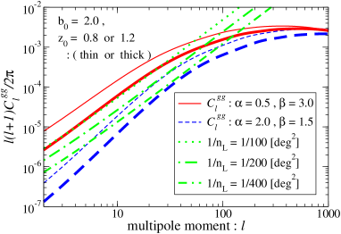
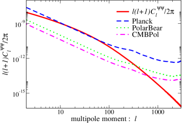
Figure 1: (Left) Angular power spectrum of the galaxy distribution, $C_{l}^{gg}$, for the Gaussian initial condition ($f_{\rm NL}=0$), and the galaxy shot noise, $1/n_{\rm L}$. We show $C_{l}^{gg}$ for various forms of galaxy sampling model [Eq. )5)], $(\alpha,~{}\beta)=(0.5,~{}3.0)$ (solid line) or ($\alpha,~{}\beta)=(2.0,~{}1.5)$ (dashed line), and $z_{0}=0.8$ (thin line) or $z_{0}=1.2$ (thick line). The dotted, dot-dashed and dash-dot-dashed lines show shot the noise contributions from $n_{\rm L}$ = 100, 200, 400 $[\rm{deg}^{-2}]$, respectively. (Right) Angular power spectrum of CMB lensing potential, $C_{l}^{\psi\psi}$ (solid line), and lensing reconstruction noise, $N_{l}^{\psi\psi}$ (non-solid lines). Each of the noise power spectrum indicates those for Planck (dashed line), PolarBear (dot-dashed) and CMBPol (dot-dash-dotted line), respectively.

III.3 Cross-Correlation: Galaxy & Lensing Potential

We focus on the linear cross-spectrum of the galaxy with the CMB lensing potential,

$$C_{l}^{\psi g}=\dfrac{2}{\pi}\int k^{2}dkP(k)\Delta_{l}^{\psi}(k)\Delta_{l}^{g}(k).$$ (17)

The most important assumption we have made so far is that the galaxy distribution and the lensing potential is linear and Gaussian. On small scales this will not be quite correct due to non-linear evolution. For simple models, fits to numerical simulation like the HALOFIT code of Ref. Smith et al. (2003) can be used to compute an approximate non-linear power spectrum. A good approximation is simply to scale the transfer functions $T(k)$ of Eq. (7), (11) so that the power spectrum has the correction from the non-linear effect

$$T(k)~{}\longrightarrow~{}T(k)\sqrt{\dfrac{P^{\rm non-linear}(k)}{P(k)}}.$$ (18)

We also include the other cross-correlation components, $C_{l}^{TE}$, $C_{l}^{T\psi}$ and $C_{l}^{Tg}$, for the estimation of the parameter errors. However, we assume that there is no cross-correlation between the polarization and the lensing potential or the galaxy distribution, $C_{l}^{E\psi}=C_{l}^{Eg}=0$. This is because the polarization is mainly produced by the Thomson scattering at the last scattering surface while the lensing potential and the galaxy distribution exist in the late-time universe. We show the angular power spectrum $C_{l}^{\psi g}$ in Fig. 2. The redshift dependence and the effect of the primordial non-Gaussianity through a scale-dependent bias are clearly seen in that figure.

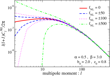
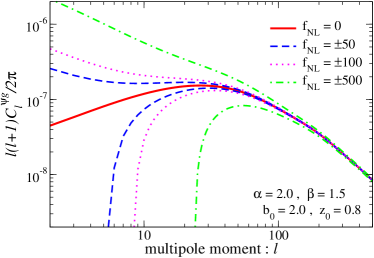
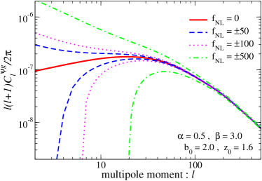
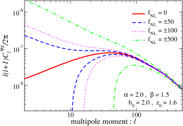
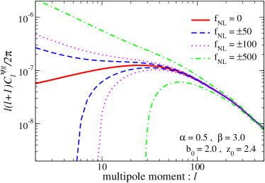
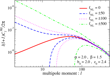
Figure 2: The cross-correlation power spectrum between the CMB lensing potential and the galaxy distribution, $l(l+1)C_{l}^{\psi g}/2\pi$ for $f_{\rm sky}=0.1$ and $N_{\rm g}=10^{6}$. The solid, dashed, dotted and dot-dashed lines correspond to $f_{\rm NL}=0,\pm 50,\pm 100,\pm 500$, respectively.

IV Modeling Galaxy Sample

We showed the analytic form of the normalized galaxy distribution function in Eq. (5). The mean redshift $z_{\rm m}$ is related to the peak redshift $z_{0}$ and determined by

$$z_{\rm m}=\int dzz\dfrac{dN}{dz}=\dfrac{z_{0}\Gamma\left[(\alpha+2)/\beta\right]}{\Gamma\left[(\alpha+1)/\beta\right]}.$$ (19)

The relation between $z_{0}$ and $z_{\rm m}$ is, for example, $z_{0}={z_{\rm m}}/0.64$ for ($\alpha$, $\beta$) = (0.5, 3.0) and $z_{0}={z_{\rm m}}/1.41$ for ($\alpha$, $\beta$) = (2.0, 1.5). In this paper, we consider a wide field survey such as the on-going Hyper Suprime-Cam (HSC) project. This is a fully funded imaging survey at Subaru telescope. The surface density $n_{\rm L}$ and the mean redshift ${z_{\rm m}}$ are related to the exposure time $t_{\exp}$ as Amara and Réfrégier (2007); Yamamoto et al. (2007),

$${z_{\rm m}} = 0.9\left(\dfrac{t_{\exp}}{\rm 30min}\right)^{0.067},$$ (20)

$$n_{\rm L} = 35\left(\dfrac{t_{\exp}}{\rm 30min}\right)^{0.44}\;{\rm[arcmin^{-2}]}.$$ (21)

In Ref. Amara and Réfrégier (2007) and Yamamoto et al. (2007), ($\alpha$, $\beta$) = (0.5, 3.0) and (2.0, 1.5) are adopted, respectively. In this paper, we adopt both cases and compare the differences between the survey models.

The validity of the above form of the galaxy distribution is shown in Ref. Yamamoto et al. (2007). They compared it with the Canada-France-Hawaii telescope (CFHT) photometric redshift data Ilbert et al. (2006). The relationship between magnitude limit and exposure time was scaled for the published Subaru Suprime-Cam specification Miyazaki et al. (2002), and these data are shown in Table 2 for the $i,g,r,z$ passbands.

The total survey area can be expressed as Yamamoto et al. (2007)

$${\rm area}=\pi\left(\dfrac{\rm field\,of\,view}{2}\right)^{2}\dfrac{T_{\rm total}}{1.1\times t_{\rm\exp}+t_{\rm op}},$$ (22)

where we assume that the field of view is 1.5^∘, the total observation time $T_{\rm total}$ is fixed as 800 hours, and the overhead time is modeled by constant, $t_{\rm op}=5$ min, plus a fraction (10%) of the exposure time $t_{\rm\exp}$ for one field of view.

$i_{\rm AB~{}limit}$	$i(S/N=10)$	$g(S/N=5)$	$r(S/N=5)$	$z(S/N=5)$
$22.97$	$1$ mins.	$3$ mins.	$1.1$ mins.	$0.3$ mins.
$23.84$	$5$ mins.	$15$ mins.	$7$ mins.	$1.4$ mins.
$24.22$	$10$ mins.	$30$ mins.	$12$ mins.	$3.5$ mins.
$24.81$	$30$ mins.	$90$ mins.	$34$ mins.	$8.1$ mins.
$25.04$	$45$ mins.	$130$ mins.	$50$ mins.	$13$ mins.

Table 2: Exposure time for the bands, $i,g,r,z$. The relation between magnitude limit and exposure time was scaled for the published Subaru Suprime-Cam specification Miyazaki et al. (2002); Yamamoto et al. (2007).

V The Fisher matrix analysis

For our Fisher matrix analysis, we refer to the method of Ref. Perotto et al. (2006) and expand it to take into account the cross-correlation between the lensing potential and the galaxy distribution. In Ref. Perotto et al. (2006), the $5\times 5$ covariance matrix is calculated for primary CMB and CMB lensing. In our case, we expand it into $8\times 8$ covariance matrix for the cross-correlation between CMB lensing and galaxy distribution.

V.1 Likelihood Function

Each data points have contributions from both signal and noise. If we assume both contributions are Gaussian distributed, we can write the likelihood function of the data given the theoretical model as

$${\cal L}({\bm{d}}|\Theta)\propto\dfrac{1}{\sqrt{{\rm det}\bar{C}(\Theta)}}\exp\left(-\frac{1}{2}\bm{d}^{\dagger}[\bar{C}(\Theta)^{-1}]\bm{d}\right),$$ (23)

where $\bm{d}=(a^{T}_{lm},a^{E}_{lm},a^{\psi}_{lm},a^{g}_{lm})$ is the data vector, $\Theta=(\theta_{1},\theta_{2},\ldots)$ is a vector describing the theoretical model parameters, and $\bar{C}(\Theta)$ is the theoretical data covariance matrix represented by both signal and noise. For it to be a good estimate, we would like it to be unbiased, $i.e.$, $\langle\Theta\rangle=\Theta_{0}$ , where $\Theta_{0}$ indicates the true parameter vector of the underlying cosmological model, $\Theta$ is the one constructed by the data vector $\bm{d}$ they minimizing the likelihood function ${\cal L}({\bm{d}}|\Theta)$ ($i.e.$, the so-called best fit model) and $\langle\ldots\rangle$ denotes an average over many independent realizations.

We can derive the effective chi-square, $\chi_{\rm eff}^{2}\equiv\sum_{XY}\sum_{lm}(-2)\ln{\cal L}$, from (23) as

$$\chi^{2}_{\rm eff}=\sum_{l}(2l+1)\left(\frac{D}{|\bar{C}|}+\ln|\bar{C}|\right),$$ (24)

where $\sum_{XY}$ represents the summation for each modes, $X,Y=\{T,E,\phi,g\}$, and $|\bar{C}|$ denotes the determinant of the theoretical data covariance matrix,

$$|\bar{C}| = (\bar{C}_{l}^{TE})^{2}(\bar{C}_{l}^{\psi g})^{2}-\bar{C}_{l}^{TT}\bar{C}_{l}^{EE}(\bar{C}_{l}^{\psi g})^{2}-\bar{C}_{l}^{\psi\psi}\bar{C}_{l}^{gg}(\bar{C}_{l}^{TE})^{2}$$ (25)

$$-\bar{C}_{l}^{EE}\bar{C}_{l}^{\psi\psi}(\bar{C}_{l}^{Tg})^{2}-\bar{C}_{l}^{EE}\bar{C}_{l}^{gg}(\bar{C}_{l}^{T\psi})^{2}+\bar{C}_{l}^{TT}\bar{C}_{l}^{EE}\bar{C}_{l}^{\psi\psi}\bar{C}_{l}^{gg}+2\bar{C}_{l}^{EE}\bar{C}_{l}^{T\psi}\bar{C}_{l}^{Tg}\bar{C}_{l}^{\psi g}~{}.$$

Here $D$ is defined as

$$D = +2\hat{C}_{l}^{TE}\bar{C}_{l}^{TE}(\bar{C}_{l}^{\psi g})^{2}+2(\bar{C}_{l}^{TE})^{2}\bar{C}_{l}^{\psi g}\hat{C}_{l}^{\psi g}$$ (27)

$$-\hat{C}_{l}^{TT}\bar{C}_{l}^{EE}(\bar{C}_{l}^{\psi g})^{2}-\bar{C}_{l}^{TT}\hat{C}_{l}^{EE}(\bar{C}_{l}^{\psi g})^{2}-2\bar{C}_{l}^{TT}\bar{C}_{l}^{EE}\bar{C}_{l}^{\psi g}\hat{C}_{l}^{\psi g}$$

$$-\hat{C}_{l}^{\psi\psi}\bar{C}_{l}^{gg}(\bar{C}_{l}^{TE})^{2}-\bar{C}_{l}^{\psi\psi}\hat{C}_{l}^{gg}(\bar{C}_{l}^{TE})^{2}-2\bar{C}_{l}^{\psi\psi}\bar{C}_{l}^{gg}\bar{C}_{l}^{TE}\hat{C}_{l}^{TE}$$

$$-\hat{C}_{l}^{EE}\bar{C}_{l}^{\psi\psi}(\bar{C}_{l}^{Tg})^{2}-\bar{C}_{l}^{EE}\hat{C}_{l}^{\psi\psi}(\bar{C}_{l}^{Tg})^{2}-2\bar{C}_{l}^{EE}\bar{C}_{l}^{\psi\psi}\bar{C}_{l}^{Tg}\hat{C}_{l}^{Tg}$$

$$-\hat{C}_{l}^{EE}\bar{C}_{l}^{gg}(\bar{C}_{l}^{T\psi})^{2}-\bar{C}_{l}^{EE}\hat{C}_{l}^{gg}(\bar{C}_{l}^{T\psi})^{2}-2\bar{C}_{l}^{EE}\bar{C}_{l}^{gg}\bar{C}_{l}^{T\psi}\hat{C}_{l}^{T\psi}$$

$$+\hat{C}_{l}^{TT}\bar{C}_{l}^{EE}\bar{C}_{l}^{\psi\psi}\bar{C}_{l}^{gg}+\bar{C}_{l}^{TT}\hat{C}_{l}^{EE}\bar{C}_{l}^{\psi\psi}\bar{C}_{l}^{gg}+\bar{C}_{l}^{TT}\bar{C}_{l}^{EE}\hat{C}_{l}^{\psi\psi}\bar{C}_{l}^{gg}+\bar{C}_{l}^{TT}\bar{C}_{l}^{EE}\bar{C}_{l}^{\psi\psi}\hat{C}_{l}^{gg}$$

$$+2\hat{C}_{l}^{EE}\bar{C}_{l}^{T\psi}\bar{C}_{l}^{Tg}\bar{C}_{l}^{\psi g}+2\bar{C}_{l}^{EE}\hat{C}_{l}^{T\psi}\bar{C}_{l}^{Tg}\bar{C}_{l}^{\psi g}+2\bar{C}_{l}^{EE}\bar{C}_{l}^{T\psi}\hat{C}_{l}^{Tg}\bar{C}_{l}^{\psi g}+2\bar{C}_{l}^{EE}\bar{C}_{l}^{T\psi}\bar{C}_{l}^{Tg}\hat{C}_{l}^{\psi g}~{}.$$

In the above expression, we have assumed that the polarization component does not correlate with the lensing potential and galaxy distribution, so we put $C_{l}^{E\psi}=C_{l}^{Eg}=0$.

On the other hand, the mock data covariance matrix $\hat{C}$ is given from the simulations and defined as $\hat{C}\equiv\langle\bm{d}\,\bm{d}^{\dagger}\rangle$. We can estimate the power spectrum of the mock data through the following definition,

$$\sum_{m}a_{lm}^{X*}a_{lm}^{Y}=(2l+1)\hat{C}_{l}^{XY}~{}.$$ (28)

From Bayes’ theorem, we assume (24) to be the distribution of theoretical data covariance matrix $\bar{C}(\Theta)$ when mock covariance matrix $\hat{C}$ is given. Then, we can account $\bar{C}$ to be a variable and $\hat{C}$ to be a constant. All expressions introduced so far assume a full sky coverage survey. However, real experiments can only see a fraction of the sky. We introduce a factor $f_{\rm sky}$, where $f_{\rm sky}$ denotes the observed fraction of the sky in the effective $\chi^{2}$. We are interested only in the confidence levels, so the normalization factor in front of the likelihood function (23) is irrelevant. We normalize as $\chi_{\rm eff}^{2}=0$ if $\bar{C}=\hat{C}$ by adding arbitrary constant and redefine $\chi_{\rm eff}^{2}$ from (24) as

$$\chi^{2}_{\rm eff}=\sum_{l}(2l+1)f_{\rm sky}\left(\frac{D}{|\bar{C}|}+\ln{\frac{|\bar{C}|}{|\hat{C}|}}-4\right),$$ (29)

and $|\hat{C}|$ denotes the determinant of the mock (observed) data covariance matrix,

$$|\hat{C}| = (\hat{C}_{l}^{TE})^{2}(\hat{C}_{l}^{\psi g})^{2}-\hat{C}_{l}^{TT}\hat{C}_{l}^{EE}(\hat{C}_{l}^{\psi g})^{2}-\hat{C}_{l}^{\psi\psi}\hat{C}_{l}^{gg}(\hat{C}_{l}^{TE})^{2}$$ (30)

$$-\hat{C}_{l}^{EE}\hat{C}_{l}^{\psi\psi}(\hat{C}_{l}^{Tg})^{2}-\hat{C}_{l}^{EE}\hat{C}_{l}^{gg}(\hat{C}_{l}^{T\psi})^{2}+\hat{C}_{l}^{TT}\hat{C}_{l}^{EE}\hat{C}_{l}^{\psi\psi}\hat{C}_{l}^{gg}+2\hat{C}_{l}^{EE}\hat{C}_{l}^{T\psi}\hat{C}_{l}^{Tg}\hat{C}_{l}^{\psi g}~{}.$$

V.2 Fisher Information Matrix

The Fisher matrix formalism can be used to understand how accurately we can estimate the values of vector of parameters ${\bm{\Theta}}$ for a given model from one or more data sets Tegmark et al. (1997). The Fisher matrix approximates the curvature of the likelihood function $\L$ around its maximum in a space spanned by the parameters $\theta$. The usual formula requires a slight generalization to account for the possibility that different surveys may only partially overlap in sky coverage as we shall show below. The likelihood function should peak at $\Theta\simeq\Theta_{0}$, and can be Taylor expanded to second order around this value. The relevant term at second order is the Fisher information matrix, defined as

$$F_{ij}\equiv\left.-\frac{\partial^{2}\ln{\mathcal{L}}}{\partial\theta_{i}\partial\theta_{j}}\right|_{\,\Theta_{0}}~{}.$$ (31)

From the Cramer-Rao inequality, the marginalized error on a given parameter $\theta_{i}$ is given by $\sigma(\theta_{i})=\sqrt{(F^{-1})_{ii}}$ for an optimal unbiased estimator such as the maximum likelihood.

Substituting equations (23) and (29) into the above expression, the Fisher information matrix is written by

$$F_{ij}=\sum_{l=2}^{l_{\rm max}}\sum_{XX^{\prime},YY^{\prime}}\frac{\partial C_{l}^{XX^{\prime}}}{\partial\theta_{i}}({\rm Cov}_{l}^{-1})_{XX^{\prime}YY^{\prime}}\frac{\partial C_{l}^{YY^{\prime}}}{\partial\theta_{j}},$$ (32)

where $i,j$ run over the cosmological parameters, $l_{\rm max}$ is the maximum multipole available given the angular resolution of the considered experiment, and $XX^{\prime},YY^{\prime}\in\{TT,EE,TE,\psi\psi,T\psi,gg,Tg,\psi g\}$. The matrix ${\rm Cov}_{l}$ is the power spectrum covariance matrix at the $l$-multipole,

$${\rm Cov}_{l}=\frac{2}{(2l+1)f_{\rm sky}}\left(\begin{array}[]{cccccccc}\Xi_{TTTT}&\Xi_{TTEE}&\Xi_{TTTE}&\Xi_{TT\phi\phi}&\Xi_{TTgg}&\Xi_{TTT\phi}&\Xi_{TTTg}&\Xi_{TT\phi g}\\ \Xi_{TTEE}&\Xi_{EEEE}&\Xi_{TEEE}&0&0&0&0&0\\ \Xi_{TTTE}&\Xi_{TEEE}&\Xi_{TETE}&0&0&0&0&0\\ \Xi_{TT\psi\psi}&0&0&\Xi_{\psi\psi\psi\psi}&\Xi_{\psi\psi gg}&\Xi_{T\psi\psi\psi}&\Xi_{Tg\psi\psi}&\Xi_{\psi\psi\psi g}\\ \Xi_{TTgg}&0&0&\Xi_{\psi\psi gg}&\Xi_{gggg}&\Xi_{T\psi gg}&\Xi_{Tggg}&\Xi_{\psi ggg}\\ \Xi_{TTT\psi}&0&0&\Xi_{T\psi\psi\psi}&\Xi_{T\psi gg}&\Xi_{T\psi T\psi}&\Xi_{T\psi Tg}&\Xi_{T\psi\psi g}\\ \Xi_{TTTg}&0&0&\Xi_{Tg\psi\psi}&\Xi_{TgTg}&\Xi_{T\psi Tg}&\Xi_{Tg\psi g}&\Xi_{Tg\psi g}\\ \Xi_{TT\psi g}&0&0&\Xi_{\psi\psi\psi g}&\Xi_{\psi ggg}&\Xi_{T\psi\psi g}&\Xi_{Tg\psi g}&\Xi_{\psi g\psi g}\end{array}\right)~{},$$ (41)

where the auto correlation coefficients are given by

$$\Xi_{TTTT} = (C_{l}^{TT})^{2}+\dfrac{2(C_{l}^{TE})^{2}\left[C_{l}^{\psi\psi}(C_{l}^{Tg})^{2}+C_{l}^{gg}(C_{l}^{T\psi})^{2}-2C_{l}^{T\psi}C_{l}^{Tg}C_{l}^{\psi g}\right]}{\left[(C_{l}^{\psi g})^{2}-C_{l}^{\psi\psi}C_{l}^{gg}\right]},$$ (42a)

$$\Xi_{EEEE} = (C_{l}^{EE})^{2},$$ (42b)

$$\Xi_{TETE} = \dfrac{1}{2}\left[(C_{l}^{TE})^{2}+C_{l}^{TT}C_{l}^{EE}\right]+\dfrac{C_{l}^{EE}\left[C_{l}^{\psi\psi}(C_{l}^{Tg})^{2}+C_{l}^{gg}(C_{l}^{T\psi})^{2}-2C_{l}^{T\psi}C_{l}^{Tg}C_{l}^{\psi g}\right]}{2\left[(C_{l}^{\psi g})^{2}-C_{l}^{\psi\psi}C_{l}^{gg}\right]},$$ (42c)

$$\Xi_{\psi\psi\psi\psi} = (C_{l}^{\psi\psi})^{2},$$ (42d)

$$\Xi_{gggg} = (C_{l}^{gg})^{2},$$ (42e)

$$\Xi_{T\psi T\psi} = \dfrac{1}{2}\left[(C_{l}^{T\psi})^{2}+C_{l}^{TT}C_{l}^{\psi\psi}\right]-\dfrac{C_{l}^{\psi\psi}(C_{l}^{TE})^{2}}{2C_{l}^{EE}},$$ (42f)

$$\Xi_{TgTg} = \dfrac{1}{2}\left[(C_{l}^{Tg})^{2}+C_{l}^{TT}C_{l}^{gg}\right]-\dfrac{C_{l}^{gg}(C_{l}^{TE})^{2}}{2C_{l}^{EE}},$$ (42g)

$$\Xi_{\psi g\psi g} = \dfrac{1}{2}\left[(C_{l}^{\psi g})^{2}+C_{l}^{\psi\psi}C_{l}^{gg}\right],$$ (42h)

while the cross-correlation ones are

$$\Xi_{TTEE} = (C_{l}^{TE})^{2},$$ (43a)

$$\Xi_{TTTE} = C_{l}^{TT}C_{l}^{TE}+\dfrac{C_{l}^{TE}\left[C_{l}^{\psi\psi}(C_{l}^{Tg})^{2}+C_{l}^{gg}(C_{l}^{T\psi})^{2}-2C_{l}^{T\psi}C_{l}^{Tg}C_{l}^{\psi g}\right]}{\left[(C_{l}^{\psi g})^{2}-C_{l}^{\psi\psi}C_{l}^{gg}\right]},$$ (43b)

$$\Xi_{TT\psi\psi} = (C_{l}^{T\psi})^{2},$$ (43c)

$$\Xi_{TTT\psi} = C_{l}^{T\psi}\left[C_{l}^{TT}-\dfrac{(C_{l}^{TE})^{2}}{C_{l}^{EE}}\right],$$ (43d)

$$\Xi_{TTgg} = (C_{l}^{Tg})^{2},$$ (43e)

$$\Xi_{TTTg} = C_{l}^{Tg}\left[C_{l}^{TT}-\dfrac{(C_{l}^{TE})^{2}}{C_{l}^{EE}}\right],$$ (43f)

$$\Xi_{TT\psi g} = C_{l}^{T\psi}C_{l}^{Tg},$$ (43g)

$$\Xi_{TEEE} = C_{l}^{TE}C_{l}^{EE},$$ (43h)

$$\Xi_{T\psi\psi\psi} = C_{l}^{T\psi}C_{l}^{\psi\psi},$$ (43i)

$$\Xi_{T\psi gg} = C_{l}^{Tg}C_{l}^{\psi g},$$ (43j)

$$\Xi_{T\psi Tg} = \dfrac{1}{2}\left(C_{l}^{T\psi}C_{l}^{Tg}+C_{l}^{TT}C_{l}^{\psi g}\right)-\dfrac{(C_{l}^{TE})^{2}C_{l}^{\psi g}}{2C_{l}^{EE}},$$ (43k)

$$\Xi_{T\psi\psi g} = \dfrac{1}{2}\left(C_{l}^{T\psi}C_{l}^{\psi g}+C_{l}^{Tg}C_{l}^{\psi\psi}\right),$$ (43l)

$$\Xi_{Tg\psi\psi} = C_{l}^{T\psi}C_{l}^{\psi g},$$ (43m)

$$\Xi_{Tggg} = C_{l}^{Tg}C_{l}^{gg},$$ (43n)

$$\Xi_{Tg\psi g} = \dfrac{1}{2}\left(C_{l}^{Tg}C_{l}^{\psi g}+C_{l}^{gg}C_{l}^{T\psi}\right),$$ (43o)

$$\Xi_{\psi\psi gg} = (C_{l}^{\psi g})^{2},$$ (43p)

$$\Xi_{\psi\psi\psi g} = C_{l}^{\psi\psi}C_{l}^{\psi g},$$ (43q)

$$\Xi_{\psi ggg} = C_{l}^{gg}C_{l}^{\psi g}.$$ (43r)

VI Forecasts

We estimate the parameter errors for Planck satellite using Fisher analysis following the method introduced in Sec. V. Our fiducial cosmology is based on the WMAP 7-year result Komatsu et al. (2010) within a flat, $\Lambda$CDM model framework.

The fiducial model parameters we consider are given as :

$$\Theta = \{~{}\Omega_{b}h^{2},~{}\Omega_{c}h^{2},~{}\Omega_{\Lambda},~{}\tau,~{}f_{\nu},~{}Y_{\rm He},~{}n_{s},~{}\Delta_{\rm R}^{2}(k_{0})\times 10^{9},~{}w_{0},~{}N_{\rm eff},~{}\alpha_{s},~{}f_{\rm NL},~{}b_{0}~{}\}$$ (44)

$$= \{0.02258,~{}0.1109,~{}0.734,~{}0.088,~{}0.02,~{}0.24,~{}0.963,~{}2.45,-1.0,~{}3.0,~{}0,~{}0,~{}2.0\},$$

where $\Omega_{b}$, $\Omega_{c}$ and $\Omega_{\Lambda}$ are the density parameters for baryon, cold dark matter and dark energy, respectively, $h$ is the Hubble constant, $\tau$ is the Thomson scattering optical depth to the last scattering surface, $f_{\nu}$ is the mass density of the massive neutrino relative to the total matter density: $f_{\nu}\equiv\Omega_{\nu}/\Omega_{m}$, $Y_{\rm He}$ is the primordial helium fraction, $n_{s}$ is spectral index of the primordial power spectrum, $\Delta_{\rm R}^{2}(k_{0})$ is the amplitude of the primordial power spectrum normalized at $k_{0}=0.002~{}{\rm Mpc^{-1}}$, $w$ is the equation of state parameter of dark energy, $N_{\rm eff}$ is the effective number of neutrinos, $\alpha_{s}$ is the running index, $f_{\rm NL}$ is the non-linear parameter which represents the primordial non-Gaussianity and $b_{0}$ is the linear bias parameter. Because we assume a flat universe the Hubble parameter is adjusted to keep our universe flat when we vary $\Omega_{\Lambda}$. For neutrino parameters, we assume the standard three neutrino species. In our analysis, the non-linear parameter $f_{\rm NL}$ and the linear bias parameter $b_{0}$ are determined by the galaxy surveys only, and the CMB experiment plays a role in breaking the parameter degeneracies. We use CAMB code Lewis et al. (2000) and HALOFIT code Smith et al. (2003) to calculate the angular power spectrum $C_{l}^{XY}$ and the non-linear region of the angular power spectrum of the galaxy distribution and lensing potential.

		CMB					galaxy		CMB $\times$ galaxy
$C_{l}^{XY}$		$C_{l}^{TT}$	$C_{l}^{EE}$	$C_{l}^{TE}$	$C_{l}^{\psi\psi}$		$C_{l}^{gg}$		$C_{l}^{T\psi}$	$C_{l}^{Tg}$	$C_{l}^{\psi g}$
$l_{\rm max}$		2500	2500	2500	1000		1000		1000	1000	1000
$f_{\rm sky}$		0.65	0.65	0.65	0.65		0.10		0.10	0.10	0.10

Table 3: Survey parameters for our calculation.

In our estimation, we include the information from temperature anisotropies, E-mode polarization and reconstructed lensing potential. The range of multipoles are $2\leq l\leq 2500$ for $C_{l}^{TT}$ and $C_{l}^{EE}$ and $2\leq l\leq 1000$ for $C_{l}^{\psi\psi}$, respectively, and survey area is taken as $f_{\rm sky}^{\rm CMB}=0.65$ for CMB survey. On the other hand, we include the information from galaxy survey, $C_{l}^{gg}$, where the range of multipoles are $2\leq l\leq 1000$ and survey area is $f_{\rm sky}^{\rm galaxy}=0.10$. We assume that there is no correlation between different patches, so that the area where there is a correlation between CMB and galaxy survey corresponds to the galaxy survey area $f_{\rm galaxy}$. We summarize the values we used mainly in the following calculation in Table 3.

The non-linear effect on the angular spectrum of the galaxy distribution begins to appear at $l\geq 100$. As the calculation of Fisher matrix assumes that all fields are random, the non-linear region of the galaxy distribution is inadequate for this calculation. However, because the auto correlation signal of the galaxy distribution is dominated by the noise term in this region as seen in Fig. 1 ($Left$), little information of the galaxy distribution from this region can be expected. Therefore, we neglect the non-linear effect of the angular power spectrum of the galaxy distribution in this paper.

Usually, the full Fisher matrix for joint experiment of galaxy survey and CMB is obtained simply by adding each Fisher matrices: $F_{ij}=F_{ij}^{CMB}+F_{ij}^{\rm galaxy}$. This method, however, does not include all the available information because it does not account for the cross-correlation of temperature-galaxy $C_{l}^{Tg}$ and lensing potential-galaxy $C_{l}^{\psi g}$. To use the angular power spectrum $C_{l}^{Tg}$ and $C_{l}^{\psi g}$ for the estimation, and make the most of the available information, we consider all of the conceivable cross-correlations and calculate the full covariance matrix, which in this case is $8{\rm\times}8$ matrix while we assume that $C_{l}^{E\psi}$ and $C_{l}^{Eg}$ are not correlated. Here, in order to account for the difference of the each survey area, and to investigate the significance of the cross-correlation signal, we calculate the full Fisher matrix of the following form,

$${\rm Case~{}(i)}~{}:~{}F_{ij} = \sum_{l=2}^{1000}F_{ij}\{f_{\rm sky}^{\rm CMB}:C_{l}^{TT},C_{l}^{EE},C_{l}^{TE},C_{l}^{\psi\psi},C_{l}^{T\psi}\}+\sum_{l=2}^{1000}F_{ij}\{f_{\rm sky}^{\rm galaxy}:C_{l}^{gg}\}$$ (45)

$$+ \sum_{l=1001}^{2500}F_{ij}\{f_{\rm sky}^{\rm CMB}:C_{l}^{TT},C_{l}^{EE},C_{l}^{TE}\},$$

$${\rm Case~{}(ii)}~{}:~{}F_{ij} = \sum_{l=2}^{2500}F_{ij}\{f_{\rm sky}^{\rm CMB}:C_{l}^{TT},C_{l}^{EE},C_{l}^{TE}\}+\sum_{l=2}^{1000}F_{ij}\{f_{\rm sky}^{\rm galaxy}:C_{l}^{\psi\psi},C_{l}^{gg},C_{l}^{\psi g}\}$$ (46)

$$+ \sum_{l=2}^{1000}F_{ij}\{f_{\rm sky}^{\rm CMB}-f_{\rm sky}^{\rm galaxy}:C_{l}^{\psi\psi}\},$$

$${\rm Case~{}(iii)}~{}:~{}F_{ij} = \sum_{l=2}^{1000}F_{ij}\{f_{\rm sky}^{\rm galaxy}:C_{l}^{TT},C_{l}^{EE},C_{l}^{TE},C_{l}^{\psi\psi},C_{l}^{T\psi},C_{l}^{gg},C_{l}^{Tg},C_{l}^{\psi g}\}$$ (47)

$$+ \sum_{l=2}^{1000}F_{ij}\{f_{\rm sky}^{\rm CMB}-f_{\rm sky}^{\rm galaxy}:C_{l}^{TT},C_{l}^{EE},C_{l}^{TE}\}+\sum_{l=1001}^{2500}F_{ij}\{f_{\rm sky}^{\rm CMB}:C_{l}^{TT},C_{l}^{EE},C_{l}^{TE}\},$$

where ”$f_{\rm sky}^{(\rm Survey)}$ ” represents the available sky fraction in the Fisher matrix with $({\rm Survey})=\{{\rm galaxy},{\rm CMB}\}$, and ”$C_{l}^{XY},\cdot\cdot\cdot$ ” denotes the angular power spectra included in the Fisher matrix with $X,Y=\{T,~{}E,~{}\psi,~{}g\}$. Case (i) does not include the cross-correlations between CMB and galaxy survey, $C_{l}^{Tg}$ and $C_{l}^{\psi g}$, and Case (ii) does not include the cross-correlations between temperature and galaxy or lensing potential, $C_{l}^{Tg}$ and $C_{l}^{T\psi}$, while Case (iii) takes account of all cross-correlations. We shall compare the difference in these three cases in the following section.

VII Result

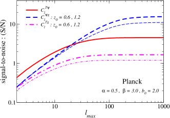
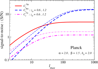
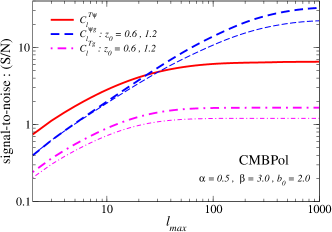
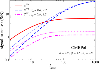
Figure 3: The signal-to-noise from $C_{l}^{T\psi}$, $C_{l}^{Tg}$ and $C_{l}^{\psi g}$, for $z_{0}$ = 0.8 (thin) and 1.2 (thick), respectively, with Planck (top) and CMBPol (bottom). The survey area and total number of the galaxies are fixed to $f_{\rm sky}=0.10$ and $N_{\rm g}=10^{6}$, respectively.

VII.1 Signal-to-Noise

The signal-to-noise ratio ($S/N$) for a cross-correlation between $X$ and $Y$ can be estimated by Peiris and Spergel (2000)

$$\left(\dfrac{S}{N}\right)^{2}=f_{\rm sky}\sum_{2}^{l_{\rm max}}(2l+1)\dfrac{(C_{l}^{XY})^{2}}{(C_{l}^{XY})^{2}+(C_{l}^{XX}+N_{l}^{XX})(C_{l}^{YY}+N_{l}^{YY})}.$$ (48)

We show the $S/N$ value in Fig. 3 where we fixed the survey area as $f_{\rm sky}=0.10$ and total number of the galaxies as $N_{\rm g}=10^{6}$, respectively. The cross-correlations between temperature and lensing potential $C_{l}^{T\psi}$ and temperature and galaxy $C_{l}^{Tg}$ are through the Integrated Sachs-Wolfe (ISW) effect imprinted in the CMB and the distribution of matter at late time. The ISW effect arise from the time-variation of the scalar metric perturbations and it is usually divided into an early ISW effect and a late ISW effect. The origin of the late ISW effect is from the time variation of the gravitational potential by the dark energy component and its effect emerges at low-multipoles. Therefore, the $S/N$ both from $C_{l}^{T\psi}$ and $C_{l}^{Tg}$ saturate around $l_{\rm max}\simeq 40$, although their amplitudes are different.

On the other hand, the cross-correlation between lensing potential and galaxy has another feature. The survey which can explore the small scale region with large $l_{\rm max}$, can get large $S/N$ from $C_{l}^{\psi g}$ more than those from $C_{l}^{T\psi}$ and $C_{l}^{Tg}$ while their amplitude is very small for the low resolution survey with small $l_{\rm max}$. The saturation of $S/N$ from $C_{l}^{\psi g}$ at large $l_{\rm max}$ for Planck in Fig. 3 (top two panels) is due to the noise contribution of the surveys. This justifies our omitting the proper modeling on small scales where non-linear evolutions are important. The signal-to-noise may be improved for high-precision future CMB survey, such as CMBPol, because it will be obtain much more information about small scale region than Planck. Since the cross-correlation between lensing potential and galaxy $C_{l}^{\psi g}$ has larger $S/N$ than other cross-correlation components, $C_{l}^{\psi g}$ would be more powerful tool when small-scale powers are observed. However, it should be noted that the correct non-linear model will be necessary on these scales.

VII.2 Parameter errors

We show the 1$\sigma$ marginalized error of each parameter in Table 4 and error contours in Fig. 4. First, we compare the analysis methods, $i.e.$, the Cases (i) - (iii) defined in Eqs. (45) - (47). From the figure we find that the cosmological parameters, such as $\Omega_{\Lambda}$, $f_{\nu}$, and $w$ are tightly constrained in Case (i), while the constraint on the non-Gaussianity parameter $f_{\rm NL}$ is tighter in Case (ii) than Case (i). Because the main difference between Case (i) and (ii) is whether one includes $C_{l}^{T\psi}$ or $C_{l}^{\psi g}$, respectively, we can conclude that the cross-correlation between lensing potential and galaxy $C_{l}^{\psi g}$ is important to determine $f_{\rm NL}$ more precisely. Assuming more high-precision CMB survey, CMBPol, the significance of $C_{l}^{\psi g}$ for constraints on $f_{\rm NL}$ are seen more clearly.

Next, we investigate how the different galaxy sampling models affect the determination of $f_{\rm NL}$. For this purpose we consider two cases, the cases ($\alpha$, $\beta$) = (0.5, 3.0) and ($\alpha$, $\beta$) = (2.0, 1.5), and the results are shown in Fig. 5. The features of the two models are that the former has a gradual distribution and the latter has a sharp one around the peak redshift $z_{0}$. Generally, the expected errors rapidly decrease with redshift $z_{0}$ for $z_{0}\lesssim 1$. As for the Case (iii) the error is almost independent of $z_{0}$ for the case with ($\alpha$, $\beta$) = (2.0, 1.5), while it has strong dependence for the case with ($\alpha$, $\beta$) = (0.5, 3.0). However, translating the peak redshift $z_{0}$ to the mean redshift ${z_{\rm m}}$, the tendency of the two models is similar to each other, although the constraint from the sharp distribution model is somewhat stronger than the gradual one, where the mean redshift ${z_{\rm m}}$ is determined by Eq. (19) and the relation between ${z_{\rm m}}$ and $z_{0}$ depends on the galaxy sampling model. For the same value of the peak redshift $z_{0}$, the gradual model represents relatively low mean redshift observation and the sharp model represents high redshift one. Therefore, the mean redshift of galaxies, rather than their distribution, determines how tight constraint one can obtain.

The difference of the constraints due to sampling models can be attributed to the degree of the correlation between the lensing potential and the galaxy distribution. Because the sharp one has narrow peak around the peak redshift, it has much large correlation with the lensing potential in this narrow range. The degree of the correlation takes maximum value at certain redshift, and it gradually decreases above the redshift. This fact reflects that $\Delta f_{\rm NL}$ slowly increases with increasing of the peak redshift above the certain redshift. On the other hand, because the gradual distribution model has a wide peak, the galaxy distribution gas the lower degree of correlation with the lensing potential, even though the correlation exists over the wider range in $k$-space. In other words, to constrain the primordial non-Gaussianity from galaxy-CMB lensing cross-correlation one should select the galaxies whose correlation with the CMB lensing potential becomes maximum.

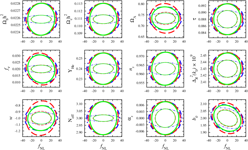
Figure 4: 1$\sigma$ confidence limits on the pair ($f_{\rm NL}$, $\theta_{i}$) in our 13-dimensional model. We show for Case (i) (dot-dashed line), Case (ii) (dashed line) and Case (iii) (solid line), respectively. We assume Planck (thick line) and CMBPol (thin line) for CMB survey, and for the galaxy survey the sky coverage and total number of galaxy sampling of $f_{\rm sky}=0.1$ and $N_{\rm g}=10^{6}$. The parameters of galaxy sampling model are fixed as $\alpha=0.5$, $\beta=3.0$ and $z_{0}=1.8$.

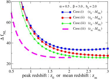
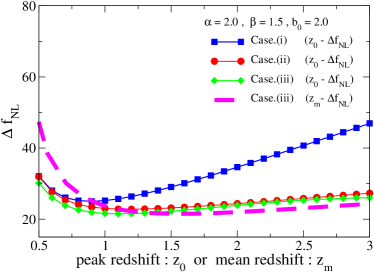
Figure 5: The comparison of the 1$\sigma$ error of $f_{\rm NL}$ in the cases with and without cross-correlations. The lines with simbols are against peak redshift $z_{0}$ and thick dashed line corresponds to the Case (iii) against mean redshift ${z_{\rm m}}$, respectively. The left panel is for the case $\alpha=0.5$, $\beta=3.0$ and the right one is for the case $\alpha=2.0$, $\beta=1.5$, in Eq.(5). Planck is considered for the CMB experiment and the galaxy survey parameters are taken as $f_{\rm sky}$ = 0.10 and $N_{\rm g}=10^{6}$.

		CMB		CMB		Case (i)				Case (ii)				Case (iii)
		No lensing		Lensing		$z_{0}=0.6$	$z_{0}=1.2$	$z_{0}=1.8$		$z_{0}=0.6$	$z_{0}=1.2$	$z_{0}=1.8$		$z_{0}=0.6$	$z_{0}=1.2$	$z_{0}=1.8$
$100\Omega_{b}h^{2}$		0.0243		0.0225		0.0225	0.0225	0.0225		0.0224	0.0225	0.0225		0.0223	0.0223	0.0224
$\Omega_{c}h^{2}$		0.00222		0.00214		0.00213	0.00214	0.00214		0.00212	0.00215	0.00216		0.00211	0.00213	0.00214
$\Omega_{\Lambda}$		0.1922		0.0530		0.0519	0.0527	0.0528		0.0635	0.0677	0.0680		0.0504	0.0526	0.0527
$\tau$		0.00553		0.00457		0.00457	0.00457	0.00457		0.00463	0.00463	0.00463		0.00456	0.00456	0.00456
$f_{\nu}$		0.0384		0.0107		0.0107	0.0106	0.0107		0.0120	0.0120	0.0121		0.0107	0.0106	0.0106
$Y_{\rm He}$		0.0159		0.0152		0.0152	0.0152	0.0152		0.0153	0.0154	0.0154		0.0151	0.0152	0.0152
$n_{s}$		0.01016		0.00937		0.00933	0.00934	0.00936		0.00926	0.00932	0.00936		0.00924	0.00929	0.00933
$\Delta_{\rm R}^{2}(k_{0})\times 10^{9}$		0.0295		0.0237		0.0237	0.0237	0.0237		0.0242	0.0243	0.0243		0.0237	0.0237	0.0237
$w$		0.651		0.197		0.191	0.195	0.195		0.253	0.269	0.270		0.187	0.195	0.195
$N_{\rm eff}$		0.135		0.116		0.116	0.116	0.116		0.116	0.117	0.117		0.116	0.116	0.116
$\alpha$		0.00841		0.00755		0.00749	0.00752	0.00754		0.00761	0.00767	0.00769		0.00745	0.00751	0.00753
$f_{\rm NL}$		—–		—–		105.7	39.9	27.0		104.9	38.3	25.9		100.8	36.9	25.1
$b_{0}$		—–		—–		0.0682	0.0718	0.0931		0.0703	0.0826	0.1076		0.0662	0.0707	0.0911

Table 4: Constraints on cosmological parameters from the Fisher matrix methods for each case. We show the marginalized 1$\sigma$ errors for the eleven-parameter or thirteen-parameter models. We assume Planck for CMB survey. For galaxy survey we assume that sky coverage and total number of galaxy sampling are $f_{\rm sky}=0.1$ and $N_{\rm g}=10^{6}$. The parameters of galaxy sampling model are taken as $\alpha=0.5$, $\beta=3.0$ for all cases.

Finally, we focus on the observing redshift dependence for the constraints on the primordial non-Gaussianit $f_{\rm NL}$. We found that the constraints on $f_{\rm NL}$ considerably depends on the mean redshift of the observations ${z_{\rm m}}$, which is related with model parameter $z_{0}$ by Eq. (19). We show its redshift dependence in Fig. 5. The errors of $f_{\rm NL}$ rapidly decrease with redshift at low redshift, $z_{0}\leq 1$, while it increases slowly at high redshift, $z_{0}\geq 1$. The effect of the primordial non-Gaussianity through the scale-dependent bias becomes large at high redshift, so that this is the reason why the smaller error of $f_{\rm NL}$ can be obtained when the higher redshift is probed. On the other hand, the auto-correlation signal of the galaxy distribution becomes small with increasing redshift. This is an opposite effect to that from the scale-dependent bias for constraint on $f_{\rm NL}$ and this is the reason why the error of $f_{\rm NL}$ gradually increases at higher redshift, in particular, in Case (i) There are two reasons for increasing of the error of $f_{\rm NL}$ at high-redshift. One is due to galaxy sampling model defined by Eq. (5). This analytic form may drop the information of the low-redshift galaxies at high $z_{0}$. The other is that the cross-correlation between lensing potential and galaxy becomes weak at high redshift $z_{0}$, as seen in Fig. 2 for $f_{\rm NL}=0$ (solid line).

Moreover, we compare the constraints from various galaxy survey conditions and linear bias parameters $b_{0}$ in Fig. 6. From this figure, we clearly see that both ”depth” and ”width” for galaxy survey are important for constraint on $f_{\rm NL}$ and what should be stressed is that the case of large bias $b_{0}$ constrains more strictly than the case of low bias. The objects with large bias are affected by the primordial non-Gaussianity more strongly than the objects with low bias, so one of the key points to put constraint on the primordial non-Gaussianity is to explore the highly biased objects. This results indicate that some galaxy survey exploring the highly biased objects could constrain $f_{\rm NL}$ in less than 10 even with Planck, for example, $\Delta f_{\rm NL}\sim~{}5$ at $z_{\rm m}=2.0$.

The estimations given above do not take into account conditions of realistic observations, because we vary only the peak redshift $z_{0}$ fixing the survey area $f_{\rm sky}$ and the available galaxy samples $N_{\rm g}$. In fact, in the real galaxy survey the survey area and the available galaxy samples will also vary due to the change of the observed mean redshift because the total observation time is finite as explained in Sec. IV. Accounting the realistic galaxy survey condition, what strategy should we develop for constraining the primordial non-Gaussianity, $e.g.$ deep survey or wide survey ? In the next section, we search for the best condition for constraining $f_{\rm NL}$.

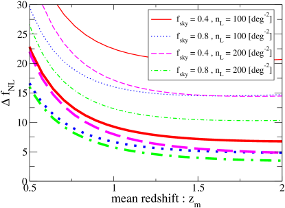
Figure 6: The 1$\sigma$ error of $f_{\rm NL}$ for wide galaxy survey with different mean redshift. We assume Planck for CMB survey, and galaxy sampling model parameters are adopted as $\alpha=0.5$, $\beta=3.0$. The thin and thick lines correspond to $b_{0}=2$ and $b_{0}=4$ cases, respectively.

VII.3 For the Galaxy Survey with Modeling

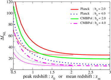
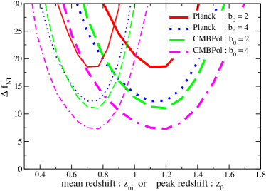
Figure 7: The 1$\sigma$ error of $f_{\rm NL}$ in the case with fixed sky coverage $f_{\rm sky}=0.1$ and total number of galaxy $N_{\rm g}=10^{6}$ (Left), and in the case with modeling for HSC survey (Right). For the CMB experiment we consider two cases. The thick lines show the errors against peak redshift $z_{0}$ and the thin lines are against mean redshift $z_{\rm m}$.

Assuming observations like HSC, we estimate a more realistic constraint on $f_{\rm NL}$ using the survey model introduced in Sec.IV. We show the results in Fig.7 and the relations between various survey parameters, namely, peak redshift $z_{0}$, survey area $f_{\rm sky}$, number density of sampling galaxy $n_{\rm L}$ and exposure time $t_{\rm exp}$ with a fixed observation time in Table 5.

In Fig. 7, we find that there is a minimal point for the error of $f_{\rm NL}$ around ${z_{\rm m}}\simeq 0.7$ and in this point, the constraints on $f_{\rm NL}$ are $\Delta f_{\rm NL}\sim~{}20$ for $b_{0}=2$ and $\Delta f_{\rm NL}\sim~{}10$ for $b_{0}=4$. From this result, the target redshift we should observe is not deep enough, in which case the surface number density of the sample galaxies is relatively small, and the observation area can be wide, $n_{\rm L}\simeq 7.0$ $[{\rm arcmin}^{-2}]$ and $f_{\rm sky}\simeq 0.35$ (at $z_{\rm m}=0.7$). (see Table 5.) For the question whether we should make wide or deep survey, the answer is that we should select the wide survey. The signal of the primordial non-Gaussianity in the scale-dependent bias $b(z,k)$ is more significant in relatively large-scale regions, as seen in Fig. 2. The noise contributions in large-scale regions are dominant by the cosmic variance due to the finiteness of survey area. On the other hand, small scale region is dominated by shot noise related to the surface number density of the galaxy samples $n_{\rm L}$, although the signal of the primordial non-Gaussianity is not sensitive there. Therefore, we conclude that the better constraining the primordial non-Gaussianity, $f_{\rm NL}$, prefers wide area survey to the deep survey. However, note that this conclusion is derived by assuming Planck and HSC experiments with a fixed observation time. Accounting for the redshift dependence of the effect of the primordial non-Gaussianity through scale-dependent bias, we should keep it in mind that the deep survey also becomes important to put a tighter constraint on $f_{\rm NL}$.

VIII Summary and Discussion

In this paper we have estimated the constraints on the cosmological parameters newly taking into account the cross-correlation between CMB lensing and galaxy angular distributions. In particular, we have focused on the constraint on the primordial non-Gaussianity through the scale-dependent bias $b(z,k)$ and estimated how much the cross-correlation between CMB lensing and galaxy would improve the constraint by the Fisher matrix analysis. In order to make the most general Fisher matrix analysis with CMB and galaxy survey experiments, we have taken into account the all the auto- and cross-correlations available which is expressed by the 8$\times$8 covariance matrix as Eq. (41). We have paid particular attention to the CMB and galaxy survey just coming up now, namely Planck satellite and HSC, and also to the future experiments like CMBPol, LSST and so on. Our estimations are mainly based on the Planck and HSC surveys, however we also show some cases for comparison when CMBPol or ambitious survey conditions are assumed.

As for the constraints on the conventional cosmological parameters, the improvement can not be expected very much from the simple estimate in which the Fisher matrices for the CMB and galaxy surveys are combined properly even if the cross-correlations are properly taken into account. However, focusing on the determination of $f_{\rm NL}$, we found that the role of the cross-correlation between CMB and galaxy is important, especially the one between CMB lensing potential and galaxy $C_{l}^{\psi g}$ contributes the determination of $f_{\rm NL}$.

We have estimated the constraints on the $f_{\rm NL}$ for the coming experiments. First, we gave the rough estimation in cases where the survey area $f_{\rm sky}$ and galaxy samples $N_{\rm g}$ are fixed and only peak redshift $z_{0}$ is varied. It was found that the keys for more strictly constraining the primordial non-Gaussianity are observing higher redshift and larger biased objects. Second, considering the realistic observations with fixed observation time, we have estimated the constraint on $f_{\rm NL}$, adapting the galaxy survey model in Ref. Yamamoto et al. (2007), which is scaled to the HSC survey. As a result we found on optimized target redshift to be $z_{0}\simeq 1$, which brings us to a conclusion that we should make a wide survey rather than a deep survey for constraining the primordial non-Gaussianity with HSC-like observation. This is because the effect of the primordial non-Gaussianity through the scale-dependent bias is significant on large scales rather than small scales. The large-scale region is dominated by the cosmic variance related to the survey area while the small-scale region is dominated by the shot noise term related to the number of the galaxy samples. Therefore, we should explore the wide survey area rather than observing a lot of galaxies. However, we should keep it in mind that high-redshift and highly-biased objects are much affected by primordial non-Gaussianity, so that the deep survey will be also essential, in the future.

The constraints on the primordial non-Gaussianity expected from HSC survey with Planck are : $\Delta f_{\rm NL}\sim~{}20$ for $b_{0}=2$ and $\Delta f_{\rm NL}\sim~{}10$ for $b_{0}=4$. Slosar et al. Slosar et al. (2008) obtained constraints on $f_{\rm NL}$ for highly biased tracers using available luminous red galaxy (LRG) or quasar (QSO) data from Sloan Digital Sky Survey (SDSS) Ho et al. (2008) and CMB data from WMAP 5, with the error of $\Delta f_{\rm NL}\sim 30$. The reason why the combination of HSC and Planck observations does not make significant improvement over the current constraints is explained as below. We have considered only 800 hours for HSC and normal galaxies. The SDSS data is obtained over longer period of time, and QSOs seem to be observed more than normal galaxies at high-redshift. These constraints are weaker than those expected with the CMB bispectrum constraints achievable with an ideal CMB experiment, $\Delta f_{\rm NL}\sim~{}{\rm few}$ (Ref. Yadav et al. (2007); Liguori and Riotto (2008)). However, the constraint on $f_{\rm NL}$ presented in this paper depends highly on the galaxy survey condition, $i.e.,$ survey area $f_{\rm sky}$, number density of sample galaxies $n_{\rm L}$ and observing peak redshift $z_{0}$. It is found that with some galaxy survey with Planck $f_{\rm NL}$ could achieve $\Delta f_{\rm NL}\sim~{}5$ at ${z_{\rm m}}=2.0$ (Fig. 6). Recently it is reported that an ambitious future galaxy survey (like the LSST survey), which provides large survey area of 30,000 ${\rm deg^{2}}$ and highly biased galaxy samples, can measure the primordial non-Gaussianity with the order $\Delta f_{\rm NL}\sim~{}2-5$ Carbone et al. (2010). The other method using the full covariance of cluster counts for Dark Energy Survey (DES) can yield $\Delta f_{\rm NL}\sim 1-5$ Cunha et al. (2010). In Ref. Carbone et al. (2010); Cunha et al. (2010), they add the Planck and galaxy survey Fisher matrices, $i.e.,$ $F_{ij}=F_{ij}^{\rm galaxy}+F_{ij}^{\rm CMB}$, and do not include the cross-correlation between CMB and galaxy survey, $i.e.,$ $C_{l}^{Tg}$ an $C_{l}^{\psi g}$, so that more tight constraint on $f_{\rm NL}$ may be expected with these cross-correlations. In any case, it is worth pursuing how well we can put a constraint on non-Gaussianity of the local-type from the large-scale structure because it contains information on non-Gaussianity at different epoch from CMB and thus the constraint through the scale-dependent bias will be an important cross check against the CMB bispectrum.

$z_{0}$	$z_{\rm m}$	$\Delta f_{\rm NL}$	$n_{\rm L}{\rm[arcmin^{-2}]}$	$f_{\rm sky}$
0.8	0.51	30.1	0.9	0.42
0.9	0.58	24.5	1.9	0.41
1.0	0.64	20.7	3.7	0.40
1.1	0.70	18.5	7.0	0.35
1.2	0.77	18.6	12.4	0.25
1.3	0.83	21.9	20.9	0.14
1.4	0.90	29.1	34.0	0.06
1.5	0.96	40.5	53.5	0.02

Table 5: The relation of parameters with fixed observation time, between the peak redshift $z_{0}$, the mean redshift $z_{\rm m}$, the $1\sigma$ error of $f_{\rm NL}$, the number density of sampling galaxy $n_{\rm L}$ and the survey area $f_{\rm sky}$, for the HSC-like survey ($b_{0}=2$).