The chemical evolution of IC10

Abstract

Context. Dwarf irregular galaxies are relatively simple unevolved objects where it is easy to test models of galactic chemical evolution.

Aims. We attempt to determine the star formation and gas accretion history of IC10, a local dwarf irregular for which abundance, gas, and mass determinations are available.

Methods. We apply detailed chemical evolution models to predict the evolution of several chemical elements (He, O, N, S) and compared our predictions with the observational data. We consider additional constraints such as the present-time gas fraction, the star formation rate (SFR), and the total estimated mass of IC10. We assume a dark matter halo for this galaxy and study the development of a galactic wind. We consider different star formation regimes: bursting and continuous. We explore different wind situations: i) normal wind, where all the gas is lost at the same rate and ii) metal-enhanced wind, where metals produced by supernovae are preferentially lost. We study a case without wind. We vary the star formation efficiency (SFE), the wind efficiency, and the time scale of the gas infall, which are the most important parameters in our models.

Results. We find that only models with metal-enhanced galactic winds can reproduce the properties of IC10. The star formation must have proceeded in bursts rather than continuously and the bursts must have been less numerous than $\sim$10 over the whole galactic lifetime. Finally, IC10 must have formed by a slow process of gas accretion with a timescale of the order of 8 Gyr.

1 Introduction

Understanding how dwarf galaxies formed is a key aspect of modern observational cosmology because they are currently the most abundant galaxy population, and were probably even more abundant during the first epochs of the Universe. In addition, according to the hierarchical formation scenario (e.g., White & Frenk white91 (1991)), they are building blocks of larger structures, hence their study is crucial to understanding galaxy formation and evolution processes. Several questions about their formation and evolution still remain unsolved, among them: i) the origin of the differences between the irregular and spheroidal morphological types (e.g., Mateo mateo98 (1998)), ii) the relation between their mass and metallicity, iii) the contribution of galactic and supernovae (SNe) winds to the evolution of the interstellar medium (ISM) metallicity, and iv) their age and star formation history (SFH) (cf., e.g., Gavilán et al. gavilan09 (2009)). Local Universe dwarf galaxies are unique environments for studying these aspects. Owing to the intrinsic faintness of dwarf galaxies, observational constraints to their evolution, such as the chemical abundances of stellar populations of different ages, can be obtained only for nearby galaxies.

Therefore, the large amount of information available for Local Group (LG) dwarf galaxies, such as star formation rate (SFR), H i and H₂ contents, star surface density, and metallicity distribution, allows us to use them to test chemical evolution models of different kind of galaxies (cf. Carigi et al. carigi02 (2002); Lanfranchi & Matteucci lanfranchi03 (2003); Mollá & Díaz molla05 (2005)). Elemental abundance ratios and their variation over cosmic time because of ongoing star formation (SF) are among the most important constraints of chemical evolution models (e.g., Mollá et al. molla96 (1996)). In this framework, optical spectroscopy of emission-line gas in galaxies is essential for deriving chemical abundances. In particular, H ii regions and planetary nebulae (PNe) provide information about the gas chemical composition at two different epochs in the galactic history: H ii regions provide the present time chemical abundances, while PNe probe the distant past chemistry.

Dwarf irregular galaxies (dIrrs) are of great interest because they enable detailed studies of issues such as the occurrence of galactic winds and the chemical enrichment of the interstellar and intergalactic media by the direct measurement of the metal content of their ISM. In addition, their low level of evolution, as implied by their low metallicity and high gas content, makes these systems the most similar to primeval galaxies and, therefore, the most useful for inferring the primordial galaxy conditions. It has also been proposed that dwarf irregulars could represent the local counterparts of faint blue galaxies found in excess in deep galaxy counts (e.g., Ellis ellis97 (1997)).

In this work, we deal with the detailed chemical evolution of the dwarf irregular galaxy IC10, building several chemical evolution models constrained by the observed properties of this galaxy. Our choice is motivated by recent observations (e.g., Sanna et al.sanna09 (2009); Magrini & Gonçalves magrini09 (2009), hereafter MG09) that place strong constraints on both its SFH and its chemical content and enrichment.

We describe the baryonic content, the SFR, and the chemical abundances of IC10 in Sect. 2. The framework of the modelling is given in Sect. 3, whereas the results are presented in Sect. 4. Finally, Sect. 5 is devoted to the conclusions.

2 Observational constraints

IC10 is a low-mass, metal-poor, and actively star-forming galaxy. It was first recognized to be an extragalactic object by Hubble (hubble36 (1936)), who defined it as ‘one of the most curious objects in the sky’. It is a member of the LG, possibly belonging to the Andromeda subgroup. Its location at low Galactic latitude implies quite uncertain determinations of its reddening (E(B-V) from 0.47 to 2.0) and distance (from 0.5 to 3 Mpc, see, e.g., Kim et al. kim09 (2009) for a summary of distances and reddenings). Distance estimates locate IC10 at around $0.7-0.8$ Mpc (e.g., Demers et al. demers04 (2004); Kniazev et al. kniazev08 (2008); Sanna et al. sanna08 (2008); Kim et al. kim09 (2009)).

Table 1: Properties of IC10

Hubble type	Irr IV	1
Distance	740 kpc	2
Dynamical mass	$\sim 1.7\times 10^{9}\leavevmode\nobreak\ M_{\odot}$	3
Stellar mass	$\sim(4-6)\times 10^{8}\leavevmode\nobreak\ M_{\odot}$	4, 5, 6
H i mass	$\sim(1.7-2.3)\times 10^{8}\leavevmode\nobreak\ M_{\odot}$	6, 7, 8, 9, 10
H2 mass	$1\times 10^{7}\leavevmode\nobreak\ M_{\odot}$	1
gas fraction	$\sim 0.22-0.36$
$\log$(O/H) + 12	$8.2-8.3$	11, 12, 13, 14, 15
$[$Fe/H$]_{\rm RGB}$	$-1.1$	16
SFRHα	$0.2\leavevmode\nobreak\ M_{\odot}$ yr-1	7, 17
SFRFIR	$0.05\leavevmode\nobreak\ M_{\odot}$ yr-1	18, 19
SFR${}_{1.4\leavevmode\nobreak\ \rm GHz}$	$0.07\leavevmode\nobreak\ M_{\odot}$ yr-1	19, 20
SFRPNe	$0.02-0.04\leavevmode\nobreak\ M_{\odot}$ yr-1	14

(1) van den Bergh (vdb00 (2000)); (2) Demers et al. (demers04 (2004)); (3) Mateo (mateo98 (1998)); (4) Jarrett et al. (jarrett03 (2003)); (5) Sakai et al. (sakai99 (1999)); (6) Vaduvescu et al. (vaduvescu07 (2007)); (7) Gil de Paz et al. (gil03 (2003)); (8) Huchtmeier et al. (huchtmeier79 (1979)); (9) Wilson et al. (wilson96 (1996)); (10) Garnett (garnett02 (2002)); (11) Lequeux et al. (lequeux79 (1979)); (12) Garnett (garnett90 (1990)); (13) Richer el al. (richer01 (2001)); (14) MG09; (15) Lozinskaya et al. (loz09 (2009)); (16) Kim et al. (kim09 (2009)); (17) Kennicutt et al. (kennicutt94 (1994)); (18) Melisse & Israel (melisse94 (1994)); (19) Bell (bell03 (2003)); (20) White & Becker (white92 (1992)).

2.1 Baryonic components

The hydrogen gas associated with IC10 extends far beyond its optical size. The inner galaxy is located within an extended, complex, and counter-rotating envelope (Huchtmeier huchtmeier79 (1979); Shostak & Skillman shostak89 (1989)) revealed by radio observations. The H i distribution has several large holes, possibly produced by SNe explosions (Wilcots & Miller wilcots98 (1998)).

Its atomic hydrogen mass has been estimated to be $M_{{\rm HI}}\sim(1.7-2.3)\times 10{{}^{8}}\leavevmode\nobreak\ M_{\odot}$ (cf. Huchtmeier huchtmeier79 (1979); Huchtmeier & Ritcher huchtmeier88 (1988); Wilson et al. wilson96 (1996); Garnett garnett02 (2002); Vaduvescu et al. vaduvescu07 (2007)) and its stellar mass to be $M_{star}=(4-6)\times 10{{}^{8}}\leavevmode\nobreak\ M_{\odot}$ (cf. Sakai et al. sakai99 (1999); Jarrett et al. jarrett03 (2003); Vaduvescu et al. vaduvescu07 (2007)). The molecular gas constitutes a small fraction of the total gas, having a mass of $M_{\rm H_{2}}\sim 1\times 10^{7}\leavevmode\nobreak\ M_{\odot}$ (van den Bergh vdb00 (2000)). Thus, its total gas fraction is $\sim 0.22-0.36$. Finally, its dynamical mass is $1.7\times 10^{9}\leavevmode\nobreak\ M_{\odot}$ (Mateo mateo98 (1998)). In Table 1, the main properties of IC10 are summarized.

2.2 The star formation rate

Several studies of IC10 have identified stellar populations with different ages (Massey & Armandroff massey95 (1995); Sakai et al. sakai99 (1999); Borissova et al. borissova00 (2000); Sanna et al. sanna08 (2008)). Deep HST colour-magnitude diagrams have uncovered both intermediate-age, red clump stars, and old red horizontal branch (RGB) stars (Sanna et al. sanna09 (2009)). Tracers of the young stellar populations are H ii regions (Hodge & Lee hodge90 (1990)) and Wolf Rayet (WR) stars (e.g., Crowther et al. crowther03 (2003)). In particular, WR stars are present in IC10 with the largest number per unit luminosity in the LG (Massey et al. massey92 (1992); Massey & Armandroff massey95 (1995)). On the other hand, the old/intermediate-age stellar populations are traced by the PNe and carbon stars (Magrini et al. magrini03 (2003); Demers et al. demers04 (2004)).

IC10 is remarkable because of its present-time high SFR. The current SFR was estimated from H$\alpha$, far-infrared (FIR), and 1.4 GHz imaging, while the intermediate age SFR was inferred from PN counting (MG09). The H$\alpha$ flux implies a SFR of $\sim 0.2\leavevmode\nobreak\ M_{\odot}$yr^-1 after an average correction for the internal extinction, but it could be as high as $0.6\leavevmode\nobreak\ M_{\odot}$yr^-1 if the largest extinction values available in the literature are adopted (Leroy et al. leroy06 (2006)). In addition, the number of WR stars provides an independent estimate of the present SFR. A comparison between the number of WRs in IC10 and a similar galaxy such as SMC– $\sim$100, among them 30 (12) confirmed spectroscopically by Crowther et al. (2003) (Massey et al. massey03 (2003)), indicates that the current SFR of IC10 is $3-4$ times higher than that of SMC, i.e., $\sim 0.5\leavevmode\nobreak\ M_{\odot}$yr^-1 (Leroy et al. leroy06 (2006)). On the other hand, the FIR and radio continuum observations infer lower estimates of the SFR ($\sim 0.05\leavevmode\nobreak\ M_{\odot}$yr^-1; Thronson et al. thronson90 (1990); White & Becker white92 (1992); Bell bell03 (2003)), probably due to the escape of UV photons or/and to a low dust content.

The mass of the stellar population that produced the observed PNe was estimated to be $1.2\times 10^{8}\leavevmode\nobreak\ M_{\odot}$ by MG09 from extended PN counting in the whole optical disk of IC10. From that, they derived a lower limit to the SFR during the period of time when IC10 PN progenitors were born, i.e. $7-10$ Gyr ago. The SFR value was estimated to be $\sim 0.02-0.04\leavevmode\nobreak\ M_{\odot}$ yr^-1.

2.3 Chemical abundances

Measuring the elemental abundances of populations with different ages are necessary to constrain the chemical evolution of a galaxy. PNe and H ii regions are useful tools in this sense, having similar spectra, and thus allowing the determination with common sets of observations and analysis techniques of the same elemental abundances.

Basically, they are representative of the ISM composition at two different epochs in the galaxy lifetime. The progenitor stars of PNe, the low- and intermediate-mass stars $1\leavevmode\nobreak\ M_{\odot}<M<8\leavevmode\nobreak\ M_{\odot}$, do not modify the composition of O, Ne, S, and Ar in the material ejected during and after the asymptotic giant branch (AGB) phase. Thus the PN abundances of these elements are characteristic of the composition of the ISM at the epoch when the PN progenitor was formed. On the other hand, He, N, and C are modified in the ejecta, because they are processed during the lifetime of the progenitor stars. In the case of IC10, the observed PNe element abundances are consistent with those of an old population. The low N/O ratios and the undetectable He ii emission lines rule out high mass progenitor stars. Therefore, their progenitor stars are of mass $M<1.2\leavevmode\nobreak\ M_{\odot}$, and were therefore born during the first half of the age of the Universe (see MG09 for details). At the same time, the chemical abundances of H ii regions are representative of the current composition of the ISM. Hence the abundances of the $\alpha$-elements, such as O, Ne, S, and Ar in H ii regions and PNe give us a quantitative measurement of the ISM chemical enrichment from the epoch of PN progenitor formation to the present.

Chemical abundances of H ii regions in IC10 have been obtained by several authors, starting with Lequeux et al. (lequeux79 (1979)), then recomputed by Skillman et al. (skillman89 (1989)), by Garnett et al. (garnett90 (1990)) with updated atomic data and ionization correction factors relative to those used by Lequeux et al. (lequeux79 (1979)), and by the spectroscopic observations of Richer et al. (richer01 (2001)). The observations by MG09 enlarged the number of studied H ii regions in whose spectra the electron temperature can be measured, and complemented them with PN observations. Spectroscopic observations of the ionized gas were obtained by Lozinskaya et al. (loz09 (2009)), who derived chemical abundances only using bright-line ratios.

The chemical abundances used to constrain our chemical evolution model are those of MG09. We adopted this uniform sample to ensure consistency between the H ii region and PN chemical abundance determinations. Moreover, the chemical abundances of H ii regions observed by MG09 in common with previous surveys agree with their determinations. The average chemical abundances of PNe and H ii regions by MG09 are reported in Table 1. In the following sections, we adopt oxygen and sulphur abundance in PNe as tracers of the past ISM composition, while we do not consider helium and nitrogen since their abundance might be altered by evolutionary processes occurring in the PN progenitors. We use the chemical abundances of H ii regions to constrain our chemical evolution models at the present time.

Table 2: Average chemical abundances of PNe and H ii regions in IC10 from MG09

	He/H	O/H($\times 10^{-4}$)	12+log(He/H)	12+log(O/H)	12+log(N/H)	12+log(S/H)	log(N/O)	log(S/O)
PNe	0.107$\pm$0.032	2.07$\pm$1.30	11.01$\pm$0.14	8.22$\pm$0.36	7.23$\pm$0.30	6.29$\pm$0.22	-1.08$\pm$0.20	-2.02$\pm$0.40
H ii regions	0.107$\pm$0.031	2.31$\pm$1.59	11.02$\pm$0.12	8.28$\pm$0.29	7.41$\pm$0.39	6.76$\pm$0.31	-0.87$\pm$0.51	-1.52$\pm$0.23

3 The chemical evolution model

The chemical evolution model adopted for IC10 is the one of Yin et al. (yin10 (2010)) which is an update of the Bradamante et al. (bradamante98 (1998)) model for dwarf irregular galaxies. In this model, we can include different SFHs, either a sequence of short starbursts followed by quiescent periods or a continuous, but very mild, star formation. The model takes into account the feedback from SNe and stellar winds giving rise to a galactic outflow when the gas thermal energy exceeds the binding energy of gas. A dark matter halo is also considered for which the dark matter is 10 times more massive than the luminous one, but roughly 3 times more extended than the luminous matter (see Yin et al. yin10 (2010) for details).

The time evolution of the fractional mass of element $i$ in the gas, $G_{i}$, is described by the equations

$$\dot{G}_{i}=-\psi(t)X_{i}(t)+R_{i}(t)+\dot{G}_{i,inf}(t)-\dot{G}_{i,out}(t),$$ (1)

where $G_{i}(t)=M_{g}(t)X_{i}(t)/M_{L}(t_{G})$ is the gas mass in the form of an element $i$ normalized to the total baryonic mass $M_{L}$ at the present day $t_{G}=13$ Gyr, $M_{g}(t)$ is the gas mass at time $t$, and $X_{i}(t)$ represents the mass fraction of element $i$ in the gas, i.e. abundance by mass. If we use the quantity $G(t)=M_{g}(t)/M_{L}(t_{G})$ to represent the total fractional mass of gas, $X_{i}(t)$ can be expressed by $G_{i}(t)/G(t)$. The four items on the right hand side of Eq. (1) represent the mass change of the element $i$ caused by the formation of new stars $\psi(t)X_{i}(t)$, the material returned by either stellar winds or SNe explosions $R_{i}(t)$, the infall of primordial gas $\dot{G}_{i,inf}(t)$, and the outflow $\dot{G}_{i,out}(t)$, respectively. The SFR $\psi(t)$ is assumed to be

$$\psi(t)=\epsilon G(t),$$ (2)

where $\epsilon$ is the star formation efficiency (SFE) expressed in unit of Gyr^-1, and is a free parameters in our work. The accretion rate of an element $i$ follows the equation

$$\dot{G}_{i,inf}(t)=X_{i,inf}Ae^{-t/\tau},$$ (3)

where $X_{i,inf}$ represents the abundances of the element $i$ in the infalling gas that we assume to be primordial (without metals), $A$ is the normalization constant constrained to reproduce the present time total mass, and $\tau$ is the accretion timescale. The rate of gas lost via galactic winds for each element is assumed to be proportional to the amount of gas present at the time $t$ given by

$$\dot{G}_{i,out}(t)=w_{i}\lambda G(t)X_{i,out}(t),$$ (4)

where $X_{i,out}(t)$, the abundance of the element $i$ in the wind, is assumed to be identical to the abundance $X_{i}(t)$ in the ISM, the parameter $\lambda$ describes the efficiency of the galactic wind and is expressed in Gyr^-1 like $\epsilon$, $w_{i}$ is the efficiency weight of each element, hence $w_{i}\lambda$ is the effective wind efficiency of the element $i$, and $\lambda$ and $w_{i}$ are the other two free parameters in our model. In this work, we have studied two kinds of winds: the normal wind and the metal-enhanced wind. In the case of the normal wind, all elements are lost in the same way, i.e., $w_{i}=1$ for all elements; however, winds, in which metals are lost preferentially relative to H and He, are referred to as “metal- enhanced” winds. The assumed initial mass function (IMF) is the Salpeter (salpeter55 (1955)) one, and the adopted stellar yields are those of Woosley & Weaver (woosley95 (1995)) for massive stars and van den Hoek & Groenewegen (van97 (1997)) for low- and intermediate-mass stars, both of which are metallicity-dependent.

4 Model results

Since we do not know a priori the SFH of IC10, we computed several models by varying the prescriptions for star formation. In particular, we developed models with either different numbers of bursts or continuous SF. We refer to the models with several bursts of duration longer than the interburst phase as models with “gasping SF”, and models with short bursts (durations shorter than 1 Gyr) as “bursting” models. The galaxy is assumed to have been formed by the continuous infall of primordial gas. In addition, we tested models with and without galactic wind.

4.1 Models without galactic winds

For comparison purposes we developed models without feedback, thus without galactic winds. In Table 3, we show the model parameters in the star-bursting and gasping cases, both without galactic winds: the SFE $\epsilon$, the time $t$ corresponding to the middle of each starburst, the duration $d$ of each burst, and the timescale for the infall $\tau$ are indicated for each model.

Table 3: Parameters of models without wind

Model	$\epsilon$	n	$t$	d	$\tau$
name	Gyr-1		Gyr	Gyr	Gyr
1	0.1	3	2/5/12.5	1/1/1	0.5
2	0.1	3	2/5/12.5	1/1/1	8
3	0.3	10	2/3/4/5/6/7/8/	0.4/0.1/…/0.1	8
			9/10.5/12.95
4	0.5	3	2/7/12.5	1/7/1	8
5	0.5	10	2/3.5/5/6.5/7.5/8.5/	0.5/0.5/…/0.5	8
			9.5/10.5/11.5/12.75

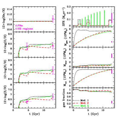
Figure 1: Time evolutions predicted by the models without winds. The left column shows the evolution of He, O, N, S abundances, the magenta points show the average abundances of PNe (open triangles, the horizontal lines from 3 to 6 Gyr denote the age range where PNe could be) and H ii regions (open circles) in Table 1; the right column shows the evolution of the total SFR, total gas mass, total stellar mass, total baryonic mass, and gas fraction, the magenta bars at 13 Gyr represent the range of the observational data (Table 1). Black-dot lines: model 1, 3 bursts with short infall timescale ($\tau=0.5$ Gyr); red-dashed lines: model 2, 3 bursts with long infall timescale ($\tau=8$ Gyr); green-solid lines: model 3, 10 bursts with long infall timescale ($\tau=8$ Gyr).

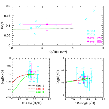
Figure 2: Abundance ratios predicted by the models without winds. The cyan squares and circles are the observed abundance of PNe and H ii regions (MG09), and the filled magenta points are their average chemical abundances (Table 1). The lines are for the same models as in Fig. 1.

Models 1 and 2, assuming that IC10 has suffered 3 bursts (2 bursts during the first half of the age of the Universe, 2 and 5 Gyr, and a third occurring roughly at the present time, namely at 12.5 Gyr) predict acceptable present-day abundances (the left column of Fig. 1), if one adopts a low SFE ($\epsilon=0.1$) and a reasonably long burst duration ($d=1$ Gyr). For a short infall timescale ($\tau=0.5$ Gyr, model 1), the abundances of different elements increase during the burst and maintain that level in the interburst phase, whereas for a long infall timescale ($\tau=8$ Gyr, model 2) the abundances decrease during the interburst phase owing to the dilution of the infalling gas, thus the present-time abundances are lower than those predicted by the fast accretion model, even if all the other parameters are the same. Since there is no SF in these models (models 1 and 2) between 5.5 and 12.0 Gyr and we do not predict the existence of stars with ages between 7.5 and 1 Gyr, at variance with observations, we compiled another model with 10 short bursts ($d\sim 0.1$ Gyr) and a long infall timescale ($\tau=8$ Gyr, to avoid a too high metallicity at the present time). This model (model 3) also shows acceptable abundance evolutionary tracks.

However, all of these models form too few stars and a lot of gas remains, hence the predicted gas fraction ($0.8-0.9$) at the present time is very high and inconsistent with the observations ($0.22-0.36$), as shown in the right column of Fig. 1. The abundance ratios (e.g., N/O, S/O) predicted by these models are consistent with the average trend of observations, but cannot explain the scatter in the data (see Fig. 2). However, the spread in the oxygen abundance of H ii regions seems to be real, and was confirmed not only by the study of MG09, but also by earlier observations (Lequeux et al. 1979, Hodge & Lee hodge90 (1990), Richer et al. richer01 (2001)). The scale-length of metallicity inhomogeneities is of $0.2-0.3$ kpc, some clumps exhibit the highest measured metallicities, and an area with a more constant metallicity, around 12+$\log$(O/H) = 8.2, being located between 0.2 to 0.5 kpc from the center (e.g. MG09).

The origin of the inhomogeneities depends on the efficiency of the mixing mechanisms in dIrrs. During the quiescent phases after the star formation episodes, the chemical elements ejected during the final stellar evolution phases cool until reaching the temperature of the ISM, and then mix with the rest of the ISM. The mixing is supposed to be homogeneous and efficient throughout the galaxy, and produced by epicyclic or radial mixing, or superbubble expansion (Roy & Kunth roy95 (1995)). However, the mixing mechanisms operating on large scales are less efficient for dIrrs because of the longer timescales of the gas mixing, and thus inhomogeneities can survive in some cases. In addition to IC10, H ii regions with different chemical compositions were observed in the dIrr galaxies WLM (Hodge & Miller 1995), NGC5253 (Kobulnicky et al. 1997), and IC 4662 (Hidalgo-Gámez et al. 2001). Weshow in Sect. 4.2.2 how models that take account of chemically enhanced winds are able to explain the observed metallicity scatter.

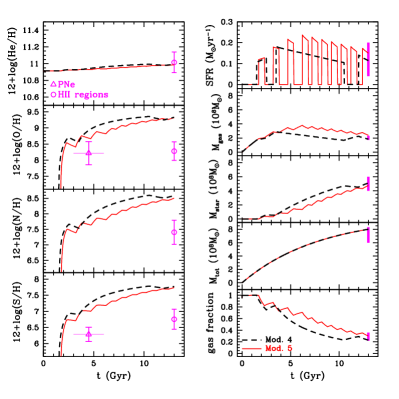
Figure 3: Time evolutions predicted by the models 4 and 5 without winds. The left column shows the evolution of He, O, N, S abundances, and the right column shows the evolution of the total SFR, total gas mass, total stellar mass, total baryonic mass, and gas fraction. The observational constraints are the same as in Fig. 1. Black-dash lines: model 4, 3 bursts with higher SFE ($\epsilon=0.5$); and red-solid lines: model 5, 10 bursts with higher SFE ($\epsilon=0.5$). Both models adopt a long infall timescale ($\tau=8$ Gyr).

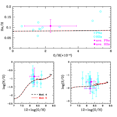
Figure 4: Abundance ratios predicted by the models 4 and 5 without winds. The points are the observed abundance of PNe and H ii regions (MG09), same as in Fig. 2. The lines are for the same models as in Fig. 3.

If we increase the SFE to consume more gas ($\epsilon=0.5$, models 4 and 5), the system reaches very high abundances, even if the long infall timescale is adopted. In Figs. 3 and  4, we show both the “gasping” and “bursting” model results. Both of them can reproduce the observed gas mass and gas fraction, but fail to reproduce most of the abundances.

4.2 Models with winds

When stellar feedback is included, galactic winds naturally develop in small galaxies. Here we describe the results of models with winds. As we have previously shown, if SFE is low the system is too gas-rich, whereas if SFE is high the system is too metal-rich. Therefore, the galactic wind should play an important role in the evolutionary history of IC10.

The rate of mass loss for the element $i$ is $w_{i}\lambda G_{i}$, where $G_{i}(t)$ is the gas mass in the form of the element $i$ normalized to the total baryonic mass at the present day, $\lambda$ is the wind efficiency and is the same for all the elements, and $w_{i}$ is the weight of the element $i$. In Table 4, we show the parameters adopted for the wind models (both normal and metal-enhanced). In particular, $w1$ and $w2$ are the models with normal winds, whereas all models labelled $mw$ have metal-enhanced winds.

4.2.1 Normal winds

In Figs. 5 and  6, we show the results for normal winds, i.e., when all the elements are lost at the same rate, as opposed to metal-enhanced winds, i.e. when metals are preferentially lost relative to H and He. In other words, in normal winds we assume that $w_{i}$ is the same for all the elements.

In this situation, since the wind blows away a large amount of gas, the total mass of infalling gas must increase to reproduce the observed total baryonic mass inside the galaxy at the present day.

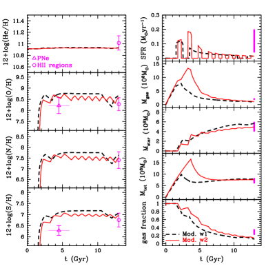
Figure 5: Time evolutions predicted by the models with normal winds. The left column shows the evolution of He, O, N, S abundances, and the right column shows the evolution of the total SFR, total gas mass, total stellar mass, total baryonic mass, and gas fraction. The observational constraints are the same as in Fig. 1. Black-dash lines: model w1, 3 bursts ($\epsilon=0.5,M_{inf}=32\times 10^{8}$ $M_{\odot}$); and red-solid lines: model w2, 10 bursts($\epsilon=0.5,M_{inf}=36\times 10^{8}$ $M_{\odot}$). Both models adopt long infall timescale ($\tau=8$ Gyr).

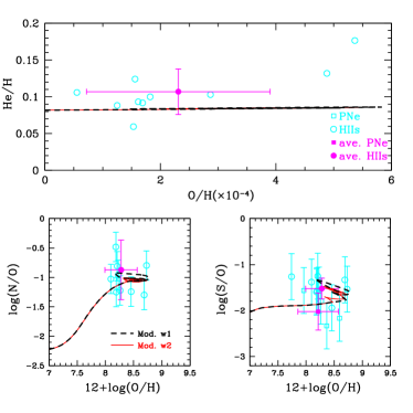
Figure 6: Abundance ratios predicted by the models with normal winds. The points are the observed abundance of PNe and H ii regions (MG09), same as in Fig. 2. The lines are for the same models as in Fig. 5.

Table 4: Parameters of models with wind ($\tau=8$ Gyr)

Model	$\epsilon$	n	$t$	d	$\lambda$	$M_{inf}$
name	Gyr-1		Gyr	Gyr	Gyr-1	$10^{8}$$M_{\odot}$
w1	0.5	3	2/7/12.5	1/7/1	1	32
w2	0.5	10	2/3.5/5/6.5/7.5/8.5/9.5/10.5/11.5/12.75	0.5/0.5/…/0.5	1	36
mw1	0.5	3	2/7/12.5	1/7/1	1	11
mw2	0.5	3	2/7/12.5	1/7/1	2	13
mw3	0.2	1	6.6	12.8	1.5	15
mw4	0.3	1	8.5	9	1.5	13
mw5	0.4	1	10	6	1.5	12
mw6	0.4	2	5/10	0.6/6	1.5	13
mw7	0.4	3	4.5/9/12.5	3/3/1	1.5	13
mw8	0.4	4	4/7/10/12.5	2/2/2/1	1.5	13
mw9	0.4	6	3/4.5/6/8/10/12.5	1/1/1/1.5/1.5/1	1.5	13
mw10	1	4	3/5/7/12.7	0.8/0.8/0.8/0.6	1.5	13
mw11	1	8	3/4/5/6/7/9/11/12.8	0.4/0.4/…/0.4	1.5	13
mw12	1	11	3/4/5/6/7/8/9/10/11/12/12.9	0.2/0.2/0.2/0.2/0.2/0.3/0.3/0.3/0.3/0.3/0.2	1.5	13

The wind efficiency is assumed to be $\lambda=1$, and both “bursting” and “gasping” models are tested (see Figs. 5 and  6). According to our models, to have a final mass of $8\times 10^{8}$$M_{\odot}$ we should accrete more than $3\times 10^{9}$$M_{\odot}$, which is 4 times higher than the present day total galactic mass. This implies that in our models an unrealistically large amount of gas is lost.

In these models, the gas infall rates are also very high, and the galaxy accumulates its mass rapidly, as we can see from the evolutionary tracks of gas mass and total baryonic mass. A large number of stars (about one third of the present stellar mass) have formed during the first star formation episode resulting in a rapid increase in metallicity at early galactic epochs. Although the enrichment is decelerated by the development of the wind, the elemental abundances are much higher than those observed in PNe. The present gas mass and gas fraction are lower than those suggested by observations because of the efficient wind. As a consequence, the star formation activity declines rapidly and reaches a very low level at the present day, in contrast to the observed value.

To summarize, the development of a normal wind implies that the galaxy should have lost an unrealistically large part of its accreted mass and been enriched very rapidly at early epochs. Therefore, it is reasonable to assume that mainly metals have been lost.

4.2.2 Metal-enhanced winds

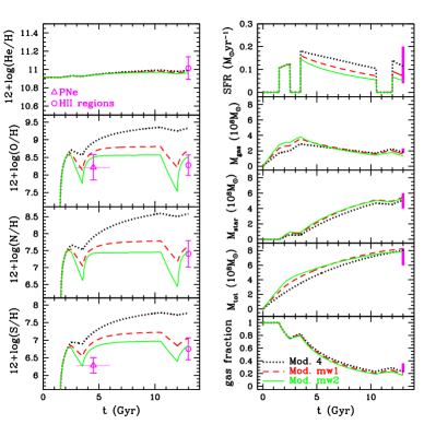
Figure 7: Time evolutions predicted by the models with metal-enhanced winds. The left column shows the evolution of He, O, N, S abundances, and the right column shows the evolution of the total SFR, total gas mass, total stellar mass, total baryonic mass, and gas fraction. The observational constraints are the same as in Fig. 1. Black-dot lines: model mw1, $\lambda=0,M_{inf}=8\times 10^{8}$$M_{\odot}$; red-dash lines: model mw2, $\lambda=1,M_{inf}=11\times 10^{8}$$M_{\odot}$; and green-solid lines: model mw3, $\lambda=2,M_{inf}=13\times 10^{8}$$M_{\odot}$.

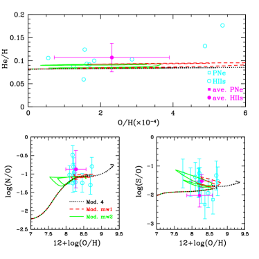
Figure 8: Abundance ratios predicted by the models with metal-enhanced winds. The points are the observed abundance of PNe and H ii regions (MG09), same as in Fig. 2. The lines are for the same models as in Fig. 7.

“Metal-enhanced” winds have been suggested by several authors (Mac Low & Ferrara mac99 (1999); D’Ercole & Brighenti dercole99 (1999); Recchi et al. recchi01 (2001); Fujita et al. fujita03 (2003); Recchi et al. recchi08 (2008)). Here, we assume that $w_{\rm H,He}=0.1,w_{\rm O,S}=0.85,w_{\rm N}=0.97$ (for this particular choice, we followed Romano et al. romano06 (2006)), which means that H and He are lost at a very low rate.

In Figs. 7 and 8, we show the results of different wind efficiencies $\lambda=0,1,2$. In Fig. 7, it is clear that the stronger the wind, the lower the metallicity, and the deeper the minima in the abundance tracks occurring in interburst time. On the other hand, the loops in the tracks in Fig. 8 are caused by the galactic wind and can explain the scatter in S/O data. However, the models are less successful in reproducing the scatter in N/O abundance ratio, especially for 12+log(O/H)$>8.2$.

Since the observed present-time oxygen abundance, 12+$\log$(O/H), is mainly between 7.9 and 8.7, implying that the wind efficiency cannot be too high, we adopted $\lambda=1.5$ in this paper. This adopted value of wind efficiency implies a reasonable amount of infalling gas ($M_{inf}=13\times 10^{8}$ $M_{\odot}$), and also provides a good fit to the observed masses, as we can see in the next section.

4.3 The effects of different SF regimes in the metal-enhanced-wind case

In this section, we describe in more detail the models with metal-enhanced wind that we developed. We tested three types of SFH: continuous SF, gasping SF, and bursting SF.

4.3.1 Continuous star formation

We developed and tested some models with continuous star formation lasting until the present time. Different SFEs were adopted. We found that if the SFE is low, the star formation duration should be long enough to form the observed number of stars (12.8 Gyr if $\epsilon=0.2$, in Figs. 9 and  10). On the other hand, if the SFE is higher, one should assume that the SF starts later and lasts for a shorter time (6 Gyr if $\epsilon=0.4$, in Figs. 9 and  10). In the former case, where SF is active since the very beginning of galaxy formation by infall, the wind begins to remove gas at earlier times (hence a higher total infall mass is required), and the metallicity increases very slowly, reaching an acceptable but low present-time value. In the latter case, since we need to reproduce the present time SFR, the star formation must have initiated $\sim$6 Gyr ago, and be very high when it begins, since the galaxy has already accreted a lot of gas. However, in this case no stars form from 7 to 10 Gyrs ago, which is inconsistent with the observations. In Fig. 10, we can see that the continuous star-formation scenario cannot explain the scatter in the metallicity data.

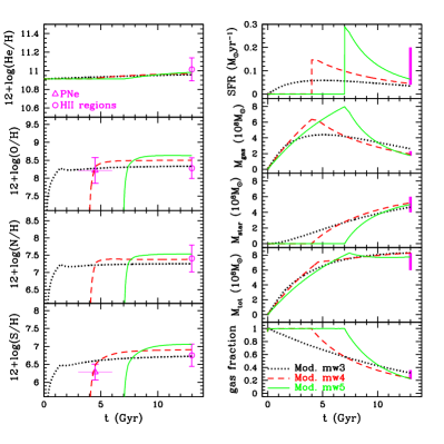
Figure 9: Time evolutions predicted by the models with continuous star formation and metal-enhanced winds. The left column shows the evolution of He, O, N, S abundances, and the right column shows the evolution of the total SFR, total gas mass, total stellar mass, total baryonic mass, and gas fraction. The observational constraints are the same as in Fig. 1. Black-dot lines: model mw3, $\epsilon=0.2,d=12.8$ Gyr; red-dash lines: model mw4, $\epsilon=0.3,d=9$ Gyr; and green-solid lines: model mw5, $\epsilon=0.4,d=6$ Gyr.

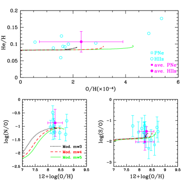
Figure 10: Abundance ratios predicted by the models with continuous star formation and metal-enhanced winds. The points are the observed abundance of PNe and H ii regions (MG09), and are the same as in Fig. 2. The lines are for the same models as in Fig. 9.

4.3.2 Gasping star formation

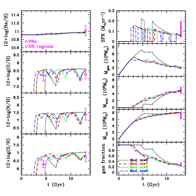
Figure 11: Time evolutions predicted by the models with gasping star formation and metal-enhanced winds. The left column shows the evolution of He, O, N, S abundances, and the right column shows the evolution of the total SFR, total gas mass, total stellar mass, total baryonic mass, and gas fraction. The observational constraints are the same as in Fig. 1. Black-dot lines: model mw6, $n=2$; red-dash lines: model mw7, $n=3$; green-solid lines: model mw8, $n=4$; and blue-dash-dot lines: model mw9, $n=6$

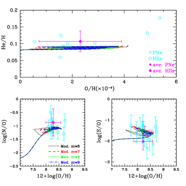
Figure 12: Abundance ratios predicted by the models with gasping star formation and metal-enhanced winds. The points are the observed abundance of PNe and H ii regions (MG09), and are the same as in Fig. 2. The lines are for the same models as in Fig. 11.

When we use the observed present SFR and gas fraction to constrain the SFE, we find that $\epsilon\sim 0.3-0.4$, if SFRs derived from FIR and 1.4 GHz measurement are used. Here we adopt $\epsilon=0.4,M_{inf}=13\times 10^{8}$ $M_{\odot}$.

In Figs. 11 and 12, we present our results for models with different numbers of bursts ($n=2$, 3, 4, 6, where the last burst is ongoing at the present day). The total duration of SF is $\sim$7 Gyr in all these 4 cases.

For model mw6 ($n=2$), the first short burst happens at 5 Gyr, then star formation halts for 2 Gyr, and restarts at $t=7$ Gyr. The first burst cannot happen too early, otherwise the minimum in metallicity (mainly caused by wind) will be too deep. In this model, we produce very few old metal-poor stars, but a bunch of metal-rich and younger stars, which does not reflect the star formation history of IC10.

In model mw7 ($n=3$), there are three bursts, one during the first half of the galactic age, one during the second half of the galactic age, and the last one which remains active at the present time; the interburst time is about 1.5 Gyr. The results are able to more closely reproduce the data.

For models mw8 ($n=4$) or mw9 ($n=6$), since the wind and the infalling gas decrease the metallicity of ISM during the interburst phase, the metal-poor stars can be formed if the galaxy experiences more star formation bursts. In these two cases, the models have more metal-poor stars formed in the first half of the galactic age and can also fit other observational data. Therefore, they are our best-fit models.

In Fig. 12, we can see that the gasping star-formation scenario can reproduce the scatter in the abundance ratios, especially in the S/O ratio, as we mentioned in Sect. 4.2.2.

4.3.3 Bursting star formation

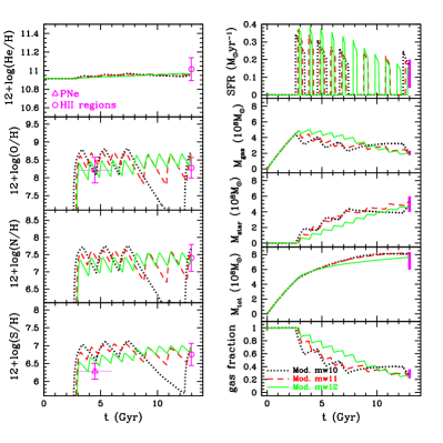
Figure 13: Time evolutions predicted by the models with bursting star formation and metal-enhanced winds.The left column shows the evolution of He, O, N, S abundances, and the right column shows the evolution of the total SFR, total gas mass, total stellar mass, total baryonic mass, and gas fraction. The observational constraints are the same as in Fig. 1. Black-dot lines: model mw10, $n=4$; red-dash lines: model mw11, $n=8$; and green-solid lines: model mw12, $n=11$.

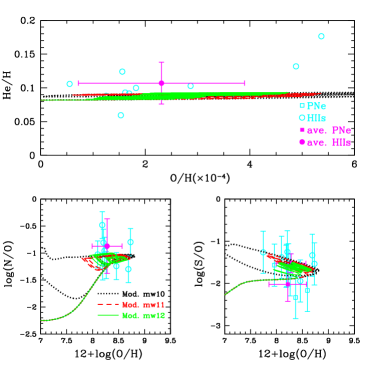
Figure 14: Abundance ratios predicted by the models models with bursting star formation and metal-enhanced winds. The points are the observed abundance of PNe and H ii regions (MG09), and are the same as in Fig. 2. The lines are for the same models as in Fig. 13.

In the gasping SF scenario, the model predicts a lot of stars whose abundances are close to the upper limit of observed PNe. Here a question arises: is it possible that IC10 is formed by short SF bursts ($d<1$ Gyr)? If this were true, the SFE should be higher than in the gasping SF scenario to form enough stars during these short bursts. We assume here that the SFE $\epsilon=1$, and that the total SF duration is around 3 Gyr in this case.

In model mw10 ($n=4$), three bursts occur in the first half of the galactic lifetime when the progenitors of PNe were born, and one occurs at the present time. A duration $d\sim 0.8$ Gyr for each burst is required to form enough stars. This leads to a relatively high metallicity after the first 3 bursts, followed by a sharp decrease in the metallicity during the long interburst period before the last burst. In this way, extremely metal-poor stars would have recently formed, at variance with observations of H ii regions, as shown in Fig. 14. To avoid these problems, we need more and shorter bursts.

In model mw11 ($n=8$), there are five bursts before $t=7$ Gyr and three bursts after. Since the interburst time is short between the first five bursts, the abundances do not decrease too much. Lots of stars form between $3-7$ Gyr and basically within the scatter of the data.

In model mw12 ($n=11$), we assume shorter bursts ($d\sim 0.2-0.3$). Stars formed between $3-6$ Gyr have metallicity consistent with the observed PNe, but in this model we still have lots of stars formed at a late age. The results of this model are consistent with observations.

Compared with the former two SF regimes, the bursting one reproduces more closely the scatter in the abundance ratios, especially for the N/O ratio when 10+log(O/H)$>$8.2, as shown in Fig 14. Therefore, model mw12 can also be considered to be among the best ones.

All these models have SFRs ($\sim 0.15-0.2$  $M_{\odot}$ yr^-1) consistent with that derived from H$\alpha$ observations, but slightly higher than the SFR obtained from FIR and 1.4GHz measurements $\sim 0.05-0.07$  $M_{\odot}$ yr^-1(see Table 1). If we were to accept the SFR value derived from H$\alpha$, then the bursting SF history might also be acceptable for IC10. On the other hand, the SFR values obtained from FIR and 1.4 GHz measurements imply that a gasping SF history is more likely.

5 Conclusions

We have studied the chemical evolution of the dwarf irregular galaxy IC10 for which detailed abundance data are now available (MG09). We have adopted a chemical evolution model for dwarf irregulars developed by Yin et al. (yin10 (2010)). This model includes detailed metallicity-dependent stellar yields for both massive and low and intermediate mass stars. The model also includes feedback from SNe and stellar winds and follows the development of galactic winds. We have explored three cases: i) no winds (no feedback); ii) normal winds, namely all the gas is lost at the same rate; and iii) metal-enhanced winds where the metals are lost preferentially relative to H and He. We also explored several regimes of star formation: a) bursting mode with short and long bursts (a regime we called “gasping SF”); and b) a continuous but low SFR.

We computed the evolutions of the abundances of several elements (He, N, O, S). The parameters of our model were: 1) the number of bursts; 2) the duration of bursts; 3) the efficiency of star formation; and 4) the efficiency of the galactic wind rate, assumed to be proportional to the amount of gas present at the time of the wind, which can vary from element to element in the case of the metal-enhanced wind.

The observational constraints were represented by the abundances and abundance ratios of the above-mentioned elements, by the present-time gas mass, the SFR, and the estimated total mass of IC10.

In spite of the large number of parameters, the number of observational constraints reproduced by our model makes us confident in concluding the following:

• The galaxy IC10 probably formed by means of a slow gas accretion process with a long infall timescale of the order of 8 Gyr.

• We do not know a priori the SFH of IC10 but our numerical simulations suggest that it should have experienced between a minimum of 4 and a maximum of 10 bursts of star formation. If we were to trust the present-time SFR measured from FIR and 1.4 GHz, the duration of the bursts should be longer than the interburst period, corresponding to a gasping mode of star formation, and the SFE should not be higher than 0.4 Gyr^-1. On the other hand, if we were to assume the present-time SFR inferred from H$\alpha$, which is higher than the other measurements, then bursts of higher SFE ($\sim 1$ Gyr^-1) but longer interburst periods can also be acceptable. In any case, we exclude a regime of continuous SF.

• We exclude evolution without galactic winds. In this case, our model can reproduce neither the present-time gas fraction nor the metallicity of IC10 at the same time without including winds. Therefore, galactic winds must occur.

• A metal-enhanced wind is more likely than a normal one, otherwise an unreasonable amount of mass is lost by the galaxy, making it impossible to fit the present-time amount of gas. In our optimal models (e.g. models mw8, mw9, and mw12), a continuous wind develops following the first burst that carries away mostly metals, as assumed in hydrodynamical simulations. Both gasping and bursting models with metal-enhanced winds can reproduce the macroscopic properties of IC10 and the scatter in the abundance ratios.

- (1) Asplund, M., Grevesse, N., & Sauval, A. J. 2005, ASPC, 336, 25
- (2) Bell, E. F. 2003, ApJ, 586, 794
- (3) Borissova, J., Georgiev, L., Rosado, M., Kurtev, R., Bullejos, A., & Valdez-Gutiérrez, M. 2000, A&A, 363, 130
- (4) Bradamante, F., Matteucci, F., & D’Ercole, A. 1998, A&A 337, 338
- (5) Carigi L., Hernandez X., & Gilmore G. 2002, MNRAS, 334, 117
- (6) Crowther, P. A., Drissen, L., Abbott, J. B., Royer, P., & Smartt, S. J. 2003, A&A, 404, 483
- (7) Demers, S., Battinelli, P., & Letarte, B. 2004, A&A 424, 125
- (8) D’Ercole, A., & Brighenti, F., 1999, MNRAS, 309, 941
- (9) Ellis, R. S. 1997, ARA&A, 35, 389
- (10) Fujita, A., Martin C. L., Mac Low, M.-M., & Abel, T. 2003, ApJ, 599, 50
- (11) Garnett, D. R. 1990, ApJ, 363, 142
- (12) Garnett, D. R. 2002, ApJ, 581, 1019
- (13) Gavilán, M., Molla, M., & Diaz, A. I. 2009, arXiv0903.0932
- (14) Gil de Paz, A., Madore, B. F., & Pevunova, O. 2003, ApJS, 147, 29
- (15) Hidalgo-Gámez, A. M., Masegosa, J., & Olofsson, K. 2001, A&A, 369, 797
- (16) Hodge, P., & Miller., B. W. 1995, ApJ, 451, 176
- (17) Hodge, P., & Lee, M. G. 1990, PASP, 102, 26
- (18) Hubble, E. 1936, The Realm of the Nebulae, New Haven: Yale University Press
- (19) Huchtmeier, W. K. 1979, A&A, 75, 170
- (20) Huchtmeier, W. K., & Ritcher, O.-G. 1988, A&A, 203, 237
- (21) Jarrett, T. H., Chester, T., Cutri, R., Schneider, S. E., & Huchra, J. P. 2003, AJ, 125, 525
- (22) Kennicutt, R. C., Jr., Tamblyn, P., & Congdon, C. E. 1994, ApJ, 435, 22
- (23) Kim, M., Kim, E., Hwang, N., Lee, M. G., Im, M., Karoji, H., Noumaru, J., & Tanaka, I. 2009, ApJ, 703, 816
- (24) Kniazev, A. Y., Pustilnik, S. A., & Zucker, D. B. 2008, MNRAS, 384, 1045
- (25) Kobulnicky, H. A., Skillman, E. D., Roy, J.-R., Walsh, J. R., & Rosa, M. R. 1997, ApJ, 477, 679
- (26) Lanfranchi G. A., & Matteucci F. 2003, MNRAS, 345, 71
- (27) Lequeux, J., Peimbert, M., Rayo, J. F., Serrano, A., & Torres-Peimbert, S. 1979, A&A, 80, 155
- (28) Leroy, A., Bolatto, A., Walter, F., & Blitz, L. 2006, ApJ, 643, 825
- (29) Lozinskaya, T. A., Egorov, O. V., Moiseev, A. V., & Bizyaev, D. V. 2009, AstL, 35, 730
- (30) Mac Low, M.-M., & Ferrara, A. 1999, ApJ, 513, 142
- (31) Magrini, L., Corradi, R. L. M., Greimel, R., Leisy, P., Lennon, D. J., Mampaso, A., Perinotto, M., Pollacco, D. L., et al. 2003, A&A, 407, 51
- (32) Magrini, L. & Gonçalves, D. R. 2009, MNRAS, 398, 280 (MG09)
- (33) Massey, P., Armandroff, T. E., & Conti, P. S. 1992, AJ, 103, 1159
- (34) Massey, P., & Armandroff, T. E. 1995, AJ, 109, 2470
- (35) Massey, P., Olsen K. A. G., & Parker, J. W. 2003, PASP, 115, 1265
- (36) Mateo M. L. 1998, ARA&A, 36, 435
- (37) Melisse, J. P. M., & Israel, F. P. 1994, A&AS, 103, 391
- (38) Mollá M., & Díaz A. I., 2005, MNRAS, 358, 521
- (39) Mollá M., Ferrini F., & Díaz A. I. 1996, ApJ, 466, 668
- (40) Recchi, S., Matteucci, F., & D’Ercole, A. 2001, MNRAS, 322, 800
- (41) Recchi, S., Spitoni, E., Matteucci, F., & Lanfranchi, G. A. 2008, A&A, 489, 555
- (42) Richer, M. G., Bullejos A., Borissova J., McCall, M. L., Lee, H., Kurtev, R., Georgiev, L., Kingsburgh, R. L., et al. 2001, A&A, 370, 34
- (43) Romano, D., Tosi, M., & Matteucci, F. 2006, MNRAS, 365, 759
- (44) Roy, J.-R., & Kunth, D. 1995, A&A, 294, 432
- (45) Sakai, S., Madore, B. F., & Freedman, W. L. 1999, ApJ, 511, 671
- (46) Salpeter, E. E. 1955, ApJ, 121, 161
- (47) Sanna, N., Bono, G., Stetson, P. B., Monelli, M., Pietrinferni, A., Drozdovsky, I., Caputo, F., Cassisi, S., et al. 2008, ApJ, 688, L69
- (48) Sanna, N., Bono, G., Stetson, P. B., Pietrinferni, A., Monelli, M., Cassisi, S., Buonanno, R., Sabbi, E., et al. 2009, ApJ, 699, L84
- (49) Shostak, G. S., & Skillman, E. D. 1989, A&A, 214, 33
- (50) Skillman, E. D., Kennicutt, R. C., & Hodge, P. W. 1989, ApJ, 347, 875
- (51) Thronson, H. A., Hunter, D. A., Casey S., & Harper, D. A. 1990, ApJ, 355, 94
- (52) Vaduvescu, O., McCall, M. L., & Richer, M. G. 2007, AJ, 134, 604
- (53) van den Bergh, S. 2000, The galaxies of the Local Group (Cambridge: Cambridge University Press)
- (54) van den Hoek, L. B., & Groenewegen, M. A. T. 1997, A&AS, 123, 305
- (55) White, R. L., & Becker, R. H. 1992, ApJS, 79, 331
- (56) White, S. D. M., & Frenk, C. S. 1991, ApJ, 379, 52
- (57) Wilcots, E. M., & Miller, B. W., 1998, AJ, 116, 2363
- (58) Wilson, C. D., Welch, D. L., Reid, I. N., Saha, A., & Hoessel, J. 1996, AJ, 111, 1106
- (59) Woosley, S. E., & Weaver, T. A., 1995, ApJS, 101, 181
- (60) Yin, J., Matteucci, F., & Vladilo, G. 2010, submitted to A&A