Two Integrals of Geodetic Lines in Oblate Ellipsoidal Coordinates

Abstract

The manuscript establishes a series expansion of the core integral that relates changes in longitude and latitude along the geodetic line in oblate elliptical coordinates, and of a companion integral which is the path length along this line as a function of latitude. The expansion is a power series in the scaled (constant) altitude of the trajectory over the surface of the ellipsoid. Each term of this series is reduced to sums over inverse trigonometric functions, square roots and Elliptic Integrals. The aim is to avoid purely numerical means of integration.

I Scope

I.1 Geodetic Coordinates

An ellipsoid is a reference surface fixed by an equatorial radius $\rho_{e}$ and a polar radius $\rho_{e}$. In many applications the second eccentricity $e$,

$$\rho_{p}^{2}=\rho_{e}^{2}(1-e^{2}),$$ (1)

is the principal reduced parameter. The three-dimensional ellipsoidal coordinates, altitude $h$ and the angles of longitude $\lambda$ and latitude $\phi$, are basically defined with the aid of a straight plumb line along the shortest distance between a general point and its “foot” point on the surface. The relation between the Cartesian geocentric coordinates $(x,y,z)$ and the curvilinear $(h,\lambda,\phi)$ is Fukushima (2006); Vermeille (2004); Jones (2004); Pollard (2002); Zhang et al. (2005); Hradilek (1976); Keeler and Nievergelt (1998),

$$\left(\begin{array}[]{c}x\\ y\\ z\\ \end{array}\right)=\left(\begin{array}[]{c}\left[N(\phi)+h\right]\cos\phi\cos\lambda\\ \left[N(\phi)+h\right]\cos\phi\sin\lambda\\ \left[N(\phi)(1-e^{2})+h\right]\sin\phi\\ \end{array}\right),$$ (2)

where

$$N(\phi)\equiv\frac{\rho_{e}}{\sqrt{1-e^{2}\sin^{2}\phi}}$$ (3)

is the distance between the foot point and the polar axis measured along the straight extension of the plumb line.

The projection $\tau$ onto the polar axis,

$$\tau\equiv\sin\phi,$$ (4)

will be useful to substitute trigonometric functions by rational functions.

I.2 Geodetic Lines

A geodetic line is the line of shortest Euclidean distance between two points within a surface of constant height $h$. This balances differential changes in the trajectory $\phi(\lambda)$ with the two principal curvatures at each point; in consequence, the meridional radius of curvature

$$M(\tau)=\frac{\rho_{e}(1-e^{2})}{(1-e^{2}\tau^{2})^{3/2}}$$ (5)

often appears to condense the notation.

The solution of the differential equations of the geodetic lines crystallizes in the integral Mathar (2007)

$$I(\tau)\equiv\int d\tau\frac{c(h+M)}{(N+h)^{2}(1-\tau^{2})\sqrt{1-\tau^{2}-\frac{c^{2}}{(N+h)^{2}}}}=\Delta\lambda,$$ (6)

which relates a difference in latitude—the limits of the integral—to a difference in longitude—the right hand side. The obliquity parameter $c$ picks an individual geodetic line out of the bundle of all lines that cross a general point. Considering the $\tau$ at which the discriminant of the root in the denominator of (6) is zero shows that $c$ is also the distance to the polar axis at the point highest above (or below) the equatorial plane Mathar (2007).

The single interest of this manuscript is in demonstrating a semi-numerical approach to evaluation of this integral. The constant of integration is tacitly fixed to imply the lower limit $\tau=\phi=0$ in the integral, because such a reference to the nodal line leads to well defined branch cuts of all square roots involved. The strategy is to expand the integrand into a power series of $h/\rho_{e}$, and to exchange the order of integration and summation, which defines a family of integrals with two additional parameters reminiscent of the order in the expansion. Each of these is reduced to the level of multiple—but finite—sums over Elliptic Integrals, assuming that these are accessible through a numerical library Carlson (1995); Carlson and Notis (1981); Bulirsch (1965, 1969).

In overview, one way of computation of (6) is addressed in Section II. Auxiliary integrals fall into two classes, one reducible to roots and inverse trigonometric functions, the other to elliptic integrals. The distance along the geodetic line defines another integral which is treated in the same spirit in Section III. Its power series yields a family of integrals which can be recast for efficient reuse of the functionality build in Section II. Finding the inverse of $I$ with respect to the parameter $c$ is closely related to the inverse problem of geodesy and shortly addressed in Section IV.

II Longitude-Latitude Coupling Integral

II.1 Taylor Expansion in Powers of Altitude

Expansion of the auxiliary $N$ and $M$ and lifting of some square roots provides a long write-up of (6),

$$I = \frac{c}{\rho_{e}}\int d\tau\frac{\frac{h}{\rho_{e}}(1-e^{2}\tau^{2})^{3/2}+1-e^{2}}{(1+\frac{h}{\rho_{e}}\sqrt{1-e^{2}\tau^{2}})(1-\tau^{2})\sqrt{1-e^{2}\tau^{2}}\sqrt{(1+\frac{h}{\rho_{e}}\sqrt{1-e^{2}\tau^{2}})^{2}(1-\tau^{2})-(c/\rho_{e})^{2}(1-e^{2}\tau^{2})}},$$ (7)

which we intend to calculate. The altitude $h$ and parameter $c$ appear only scaled with $\rho_{e}$, so introducing a function of two dimensionless variables $h$ and $c$,

$$I_{\alpha}(h,c)\equiv\int d\tau\frac{(1-e^{2}\tau^{2})^{\alpha}}{(1+h\sqrt{1-e^{2}\tau^{2}})(1-\tau^{2})\sqrt{(1+h\sqrt{1-e^{2}\tau^{2}})^{2}(1-\tau^{2})-c^{2}(1-e^{2}\tau^{2})}},$$ (8)

shows the composition

$$I=\frac{c}{\rho_{e}}\left[\frac{h}{\rho_{e}}I_{1}(\frac{h}{\rho_{e}},\frac{c}{\rho_{e}})+(1-e^{2})I_{-1/2}(\frac{h}{\rho_{e}},\frac{c}{\rho_{e}})\right].$$ (9)

The structure of the integrand is dominated by the two variables

$$T\equiv 1-\tau^{2};\quad E\equiv 1-e^{2}\tau^{2}.$$ (10)

The power series of (8) becomes

$$I_{\alpha}(h,c)=\sum_{s=0}^{\infty}(-h)^{s}\sum_{k=0}^{s}\kappa_{s,k}\int d\tau\frac{E^{\alpha+s/2}}{(T-c^{2}E)^{k+1/2}}T^{k-1}.$$ (11)

The coefficients $\kappa$ emerge from the product of the geometric series of $1/(1+hE^{1/2})$ by the binomial expansion of $1/\sqrt{(1+hE^{1/2})^{2}T-c^{2}E}$ in (8):

$$\kappa_{s,k}=4^{k}\binom{-1/2}{k}\sum_{l=k}^{\min(2k,s)}\binom{k}{l-k}(-1/2)^{l}=(-1)^{k}\binom{-1/2}{k}+(-1)^{s}2^{2k-s-1}\binom{-1/2}{k}P_{2k-s-1}^{(1+s-k,-k)}(0).$$ (12)

The term with the Jacobi Polynomial $P$ is to be interpreted as zero if $k\leq s/2$.

$s\backslash k$	0	1	2	3	4	5	6	7	8	9
0	1
1	1	1
2	1	1/2	3/2
3	1	1/2	0	5/2
4	1	1/2	3/8	-5/4	35/8
5	1	1/2	3/8	5/8	-35/8	63/8
6	1	1/2	3/8	5/16	35/16	-189/16	231/16
7	1	1/2	3/8	5/16	0	63/8	-231/8	429/16
8	1	1/2	3/8	5/16	35/128	-63/32	1617/64	-2145/32	6435/128
9	1	1/2	3/8	5/16	35/128	63/128	-693/64	4719/64	-19305/128	12155/128

Table 1: Table of the rational values of $\kappa_{s,k}$ by equation (12). Each column attains a constant value for rows $s\geq 2k$.

(11) states the problem in terms of integrals

$$I_{\beta,k}\equiv\int d\tau\frac{T^{k-1}E^{\beta}}{(T-c^{2}E)^{k+1/2}}=\int d\tau\frac{(1-\tau^{2})^{k-1}(1-e^{2}\tau^{2})^{\beta}}{[1-\tau^{2}-c^{2}(1-e^{2}\tau^{2})]^{k+1/2}}.$$ (13)

for $\beta=\alpha+s/2=-1/2,0,1/2,1,3/2,\ldots$ and $k=0,1,2,3,\ldots$. For small eccentricities, the $I_{\beta,k}$ are nearly independent of $\beta$ because $E$ is close to unity, so it suffices to illustrate the values for zero lower limit and variable upper limit $\tau$ for one value of $\beta$ in Figure 1.

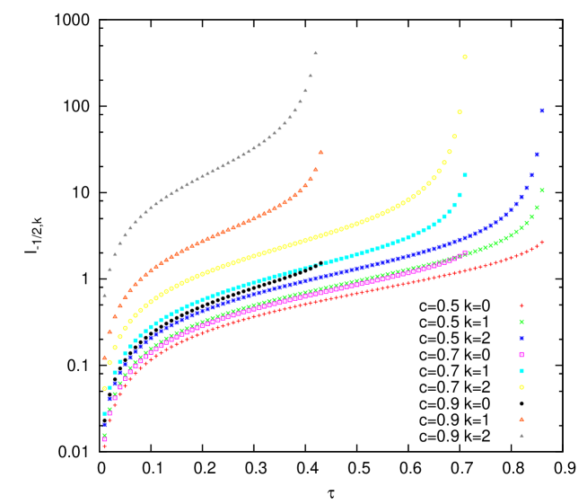
Figure 1: Values of $I_{-1/2,k}$ with a lower limit of $\tau=0$ for three different $c$ and three different $k$ with $e=0.08182$. Small $c$ indicates near-polar routes where the branch cut with $I_{\beta,k}\to\infty$ is at larger $\tau$.

The main disadvantage of the method is that the eventual constancy of $\kappa_{s,k}$ down the columns of Table 1 in conjunction with the alternating sign of $(-h)^{s}$ in (11) induces oscillatory behavior (cancellation effects) of the series if $h$ is not small.

For integrals classifications, (13) is phrased as

$$I_{\beta,k}=\frac{e^{2\beta}}{(1-c^{2}e^{2})^{k+1/2}}\int_{0}d\tau\frac{(1-\tau^{2})^{k-1}(a^{2}-\tau^{2})^{\beta}}{(b^{2}-\tau^{2})^{k+1/2}},$$ (14)

where two parameters $a$ and $b$,

$$a\equiv 1/e^{2}>b\equiv(1-c^{2})/(1-c^{2}e^{2}),$$ (15)

decide on the branches of the Elliptic Integrals. The exponent $\beta$ either leads to reduction to elementary functions if it is an integer (Section II.2), or to Elliptic Integrals if it is half-integer (Section II.3).

II.2 Cases of Elementary Functions

If $\beta=0,1,2,..$ and $k>0$, we substitute $x=\tau^{2}$ in (14),

$$I_{\beta,k}=\frac{e^{2\beta}}{2(1-c^{2}e^{2})^{k+1/2}}\int_{0}dx\frac{(1-x)^{k-1}(a^{2}-x)^{\beta}}{\sqrt{x}(b^{2}-x)^{k+1/2}},$$ (16)

equivalent to the computation of

$$J_{\beta,k}(x)\equiv\int dx\frac{(1-x)^{k-1}(a^{2}-x)^{\beta}}{\sqrt{x}(b^{2}-x)^{k+1/2}}.$$ (17)

Partial integration of this integral generates the recurrence

$$\left[1+2\beta+\frac{2(k-1)b^{2}+2k+1}{b^{2}-1}\right]J_{\beta,k}=2\sqrt{x}\frac{(1-x)^{k-1}(a^{2}-x)^{\beta}}{(b^{2}-x)^{k+1/2}}+2\frac{k-1}{b^{2}-1}J_{\beta,k-1}$$

$$+2a^{2}\beta J_{\beta-1,k}+(2k+1)\frac{b^{2}}{b^{2}-1}J_{\beta,k+1}.$$ (18)

This allows to build the entire table of $J_{\beta,k}$ from a list of $J_{\beta,0}$, $J_{\beta,1}$ and $J_{0,k}$.

The substitution

$$z=\frac{1}{b^{2}-x},\quad x=b^{2}-\frac{1}{z}$$ (19)

and binomial expansion establish

$$J_{\beta,k} = \int dz\frac{[(1-b^{2})z+1]^{k-1}}{\sqrt{b^{2}z-1}}\frac{[(a^{2}-b^{2})z+1]^{\beta}}{z^{\beta}}$$ (20)

$$= \sum_{s=0}^{k-1}\binom{k-1}{s}\sum_{m=0}^{\beta}\binom{\beta}{m}(1-b^{2})^{s}(a^{2}-b^{2})^{m}\int dz\frac{z^{s+m-\beta}}{\sqrt{b^{2}z-1}},\quad k\geq 1,\quad\beta\geq 0.$$ (21)

• The special case $s+m-\beta=0$ is covered by

  $$\int\frac{dz}{\sqrt{cz-1}}=\frac{2}{c}\sqrt{cz-1}.$$ (22)

• The cases $s+m-\beta<0$ are handled by (Gradstein and Ryshik, 1981, 2.245.2)

  $$\int\frac{dz}{z^{t+1}\sqrt{cz-1}}=c^{t}\frac{\Gamma(t+1/2)}{\Gamma(t+1)}\left[\sqrt{cz-1}\sum_{l=0}^{t-1}\frac{\Gamma(l+1)}{\Gamma(3/2+l)}\frac{1}{(cz)^{l+1}}+2\frac{1}{\sqrt{\pi}}\arctan\sqrt{cz-1}\right],\quad t\geq 0.$$ (23)

  The sum evaluates to zero if the upper limit is smaller than the lower limit.

• The cases $s+m-\beta\geq 0$ are solved by (Gradstein and Ryshik, 1981, 2.222)

  $$\int\frac{z^{t}}{\sqrt{cz-1}}dz=\frac{2\sqrt{cz-1}}{c^{t+1}}\sum_{l=0}^{t}\binom{t}{l}\frac{(cz-1)^{l}}{2l+1},\quad t\geq 0.$$ (24)

This has effectively written (21) as triple sums. [In numerical practice, the integral in (21) is placed into a look-up table for the $\beta+k$ different values of the exponent $s+m-\beta$.] The case $\beta=0$ appears as a double sum, but is recast into a single sum by resummation of the $l$-sum in (24) and the $s$-sum in (21):

$$J_{0,k} = 2\frac{1}{b^{2k}}\sqrt{b^{2}z-1}\sum_{l=0}^{k-1}\binom{k-1}{l}(1-b^{2})^{l}\frac{(b^{2}z-1)^{l}}{2l+1}$$ (25)

$$= 2\frac{\sqrt{b^{2}z-1}}{b^{2k}}{}_{2}F_{1}\left(\frac{1}{2},1-k;\frac{3}{2};(b^{2}-1)(b^{2}z-1)\right)=2\frac{\sqrt{x}}{b^{2k}\sqrt{b^{2}-x}}{}_{2}F_{1}\left(\frac{1}{2},1-k;\frac{3}{2};\frac{(1-b^{2})x}{b^{2}-x}\right).$$ (26)

The remaining part of Section II.2 considers the case $k=0$ which is not available from (21):

$$I_{\beta,0} = \frac{e^{2\beta}}{2\sqrt{1-c^{2}e^{2}}}\int d\tau\frac{(a^{2}-\tau^{2})^{\beta}}{(1-\tau^{2})\sqrt{b^{2}-\tau^{2}}}$$ (27)

$$= \frac{e^{2\beta}}{2\sqrt{1-c^{2}e^{2}}}\sum_{l=0}^{\beta}\binom{\beta}{l}(a^{2}-1)^{\beta-l}\int d\tau\frac{(1-\tau^{2})^{l-1}}{\sqrt{b^{2}-\tau^{2}}}$$

$$= \frac{e^{2\beta}}{2\sqrt{1-c^{2}e^{2}}}(a^{2}-1)^{\beta}\left[\frac{1}{2\sqrt{1-b^{2}}}\arccos\frac{b^{2}(1+\tau^{2})_{2}\tau^{2}}{b^{2}(1-\tau^{2})}+\sum_{l=1}^{\beta}\binom{\beta}{l}\frac{1}{(a^{2}-1)^{l}}\int d\tau\frac{(1-\tau^{2})^{l-1}}{\sqrt{b^{2}-\tau^{2}}}\right].$$

[The split value at $l=0$ is derived substituting $y=1/(1-\tau^{2})$, then using (Gradstein and Ryshik, 1981, 2.261). The constant of integration is chosen to realize the limit $I_{0,0}\stackrel{{\scriptstyle\tau\to 0}}{{\longrightarrow}}0$.]

This is a superposition of

$$\int d\tau\frac{(1-\tau^{2})^{l-1}}{\sqrt{b^{2}-\tau^{2}}}=\sum_{i=0}^{l-1}\binom{l-1}{i}(1-b^{2})^{l-1-i}\int d\tau(b^{2}-\tau^{2})^{i-1/2}=\sum_{i=0}^{l-1}\binom{l-1}{i}(1-b^{2})^{l-1-i}B_{i},$$ (28)

where we have defined

$$B_{i}\equiv\int d\tau(b^{2}-\tau^{2})^{i-1/2};\quad i=0,1,2,.\dots$$ (29)

Starting from

$$B_{0} = \arcsin\frac{\tau}{b},$$ (30)

the recurrence (Gradstein and Ryshik, 1981, 2.260.2)

$$B_{i}=\frac{\tau}{2i}(b^{2}-\tau^{2})^{i-1/2}+\left(1-\frac{1}{2i}\right)b^{2}B_{i-1}$$ (31)

allows to calculate (28) and eventually (27).

II.3 Elliptic case

This section looks at (14) for the cases $\beta=-\frac{1}{2}$, $\frac{1}{2}$, $\frac{3}{2}$, $\frac{5}{2}\ldots$. Let

$$\bar{J}_{\beta,k}(\tau)\equiv 2\int d\tau\frac{(1-\tau^{2})^{k-1}(a^{2}-\tau^{2})^{\beta}}{(b^{2}-\tau^{2})^{k+1/2}}.$$ (32)

The factor 2 in the definition is chosen to maintain the “alignment” $\bar{J}_{\beta,k}(\tau)=J_{\beta,k}(\tau^{2})$. Partial integration offers the recurrence

$$\left[1+2\beta+\frac{2(k-1)b^{2}+2k+1}{b^{2}-1}\right]\bar{J}_{\beta,k}=2\tau\frac{(1-\tau^{2})^{k-1}(a^{2}-\tau^{2})^{\beta}}{(b^{2}-\tau^{2})^{k+1/2}}+2\frac{k-1}{b^{2}-1}\bar{J}_{\beta,k-1}$$

$$+2a^{2}\beta\bar{J}_{\beta-1,k}+(2k+1)\frac{b^{2}}{b^{2}-1}\bar{J}_{\beta,k+1},$$ (33)

which is the same as (18).

For $k\geq 1$, binomial expansion of the numerator in (32) proposes

$$\bar{J}_{\beta,k}=2\sum_{s=0}^{k-1}\sum_{m=0}^{\beta+1/2}\binom{k-1}{s}(1-b^{2})^{s}\binom{\beta+1/2}{m}(a^{2}-b^{2})^{m}\int\frac{d\tau}{\sqrt{(a^{2}-\tau^{2})(b^{2}-\tau^{2})}(b^{2}-\tau^{2})^{1+s-(\beta+1/2-m)}}.$$ (34)

These elliptic integrals with integer exponents $v\equiv 1+s-(\beta+1/2-m)\geq 0$ are (Byrd and Friedman, 1971, 219.06)

$$\int d\tau\frac{1}{\sqrt{(a^{2}-\tau^{2})(b^{2}-\tau^{2})}(b^{2}-\tau^{2})^{v}}=\frac{1}{ab^{2v}}D_{2v},$$ (35)

where (Byrd and Friedman, 1971, 313.05)(Gradstein and Ryshik, 1981, 3.158.15)

$$D_{0} = F(\xi,b/a),$$ (36)

$$D_{2} = F(\xi,b/a)+\frac{a^{2}}{a^{2}-b^{2}}\left[\frac{\tau}{a}\frac{\sqrt{a^{2}-\tau^{2}}}{\sqrt{b^{2}-\tau^{2}}}-E(\xi,b/a)\right],$$ (37)

with $\sin\xi\equiv\tau/b$. [In this equation and where used with two arguments, (45), (56) and the last equation in the appendix, $E$ is the incomplete Elliptic Integral of the second kind, elsewhere the shorthand (10).] The recurrence extending these two values both sides to larger or negative $v$ is (Byrd and Friedman, 1971, 313.05)

$$(2v+1)(a^{2}-b^{2})D_{2v+2}=(2v-1)b^{2}D_{2v-2}+2v(a^{2}-2b^{2})D_{2v}+a\sqrt{a^{2}-\tau^{2}}\frac{\tan\xi}{\cos^{2v}\xi}.$$ (38)

Similar to the exception in Section II.2, the case $k=0$ is not covered by the expansion above and established individually:

$$\bar{J}_{\beta,0} = 2\int d\tau\frac{(a^{2}-\tau^{2})^{\beta}}{(1-\tau^{2})\sqrt{b^{2}-\tau^{2}}}$$ (39)

$$= 2\int d\tau\frac{(a^{2}-\tau^{2})^{\beta+1/2}}{(1-\tau^{2})\sqrt{(a^{2}-\tau^{2})(b^{2}-\tau^{2})}}$$ (40)

$$= 2\sum_{m=0}^{\beta+1/2}\binom{\beta+1/2}{m}(a^{2}-1)^{\beta+1/2-m}\int d\tau\frac{(1-\tau^{2})^{m-1}}{\sqrt{(a^{2}-\tau^{2})(b^{2}-\tau^{2})}}.$$ (41)

The term $m=0$ is an Elliptic Integral of the third kind (Byrd and Friedman, 1971, 219.02)(Gradstein and Ryshik, 1981, 3.157.7):

$$\int d\tau\frac{1}{(1-\tau^{2})\sqrt{(a^{2}-\tau^{2})(b^{2}-\tau^{2})}}=\frac{1}{a}\Pi(\xi,b^{2},b/a).$$ (42)

Because the case $k=s=0$ with $\beta=-1/2$ is the only contribution to (11) and (8) if the geodetic line is on the surface of the ellipsoid ($h=0$), this is the only value relevant to the integral (7) for this “classic” case.

The terms $m\geq 1$ are delegated to (Byrd and Friedman, 1971, 219.05) by binomial expansion of the numerator,

$$\int d\tau\frac{(1-\tau^{2})^{m-1}}{\sqrt{(a^{2}-\tau^{2})(b^{2}-\tau^{2})}}=\sum_{l=0}^{m-1}\binom{m-1}{l}\frac{(-b^{2})^{l}}{a}A_{2l}.$$ (43)

Starting from (Byrd and Friedman, 1971, 310.02,310.05)

$$A_{0} = F(\xi,b/a);$$ (44)

$$b^{2}A_{2} = a^{2}[F(\xi,b/a)-E(\xi,b/a)],$$ (45)

more values of $b^{2l}A_{2l}$ may be generated from the recurrence (Byrd and Friedman, 1971, 310.05)

$$(2l+1)b^{2l+2}A_{2l+2}=a\sqrt{b^{2}-\tau^{2}}\sqrt{a^{2}-\tau^{2}}+2l(a^{2}+b^{2})b^{2l}A_{2l}+(1-2l)a^{2}b^{2l}A_{2l-2};\quad l\geq-1.$$ (46)

III Line Distance Integral

III.1 Reduction to the Angular Coupling Integral

The formula for the distance $s$ along the geodetic line is given by Mathar (2007)

$$s = \int d\tau\frac{h(1-e^{2}\tau^{2})+N(1-e^{2})}{(1-e^{2}\tau^{2})\sqrt{1-\tau^{2}-\frac{c^{2}}{(N+h)^{2}}}}$$ (47)

$$= \rho_{e}\int d\tau\frac{(1+\frac{h}{\rho_{e}}E^{1/2})\frac{h}{\rho_{e}}E^{3/2}+1-e^{2}+\frac{h}{\rho_{e}}(1-e^{2})E^{1/2}}{E^{3/2}\sqrt{(1+\frac{h}{\rho_{e}}E^{1/2})^{2}T-\frac{c^{2}}{\rho_{e}^{2}}E}}$$ (48)

$$= \rho_{e}\left[\frac{h}{\rho_{e}}S_{0}(\frac{h}{\rho_{e}},\frac{c}{\rho_{e}})+(\frac{h}{\rho_{e}})^{2}S_{1/2}(\frac{h}{\rho_{e}},\frac{c}{\rho_{e}})+(1-e^{2})S_{-3/2}(\frac{h}{\rho_{e}},\frac{c}{\rho_{e}})+\frac{h}{\rho_{e}}(1-e^{2})S_{-1}(\frac{h}{\rho_{e}},\frac{c}{\rho_{e}})\right],$$ (49)

calling a group of integrals

$$S_{\alpha}(h,c)\equiv\int d\tau\frac{E^{\alpha}}{\sqrt{T+2hE^{1/2}T+h^{2}ET-c^{2}E}}$$ (50)

with two dimensionless scaled parameters and one characteristic exponent $\alpha$. Binomial expansion of the square root provides a power series in $h$,

$$S_{\alpha}(h,c)=\sum_{s=0}^{\infty}h^{s}\sum_{k=\lceil s/2\rceil}^{s}\binom{-1/2}{k}\binom{k}{s-k}2^{2k-s}\int d\tau\frac{E^{\alpha+s/2}T^{k}}{(T-c^{2}E)^{k+1/2}}.$$ (51)

The integral is similar to (13); the difference is a factor $T$ plus the request from (49) to evaluate the cases $\alpha=-3/2$ and $\alpha=-1$. The factor $T$ is distributed with the aid of

$$T=1-\frac{1}{e^{2}}+\frac{1}{e^{2}}E.$$ (52)

Recalling (15), this maps (51) on the integrals (13)

$$\int d\tau\frac{E^{\alpha+s/2}T^{k}}{(T-c^{2}E)^{k+1/2}}=(1-a)I_{\alpha+s/2,k}+aI_{\alpha+1+s/2,k}.$$ (53)

III.2 Special Values

To carry out the right hand side of (53), the only aspect not yet covered by Section II is to implement $I_{-3/2,k}$ and $I_{-1,k}$. Furthermore, $k$ is only required for the restricted range of $s$ seen in the summation (51), which reduces the “new” cases further to

• $I_{-3/2,0}$ from $(s,k,\alpha)=(0,0,-3/2)$,

• $I_{-1,0}$ from $(s,k,\alpha)=(0,0,-1)$,

• and $I_{-1,1}$ from $(s,k,\alpha)=(1,1,-3/2)$,

because otherwise the first index of $I_{\beta,k}$ is $\beta\geq-1/2$, already treated in Section II. Turning to

$$I_{-3/2,0}=\frac{e^{-3}}{(1-c^{2}e^{2})^{1/2}}\int d\tau\frac{1}{(1-\tau^{2})(a^{2}-\tau^{2})^{3/2}(b^{2}-\tau^{2})^{1/2}}$$ (54)

proposes partial fraction decomposition

$$\int d\tau\frac{1}{(1-\tau^{2})(a^{2}-\tau^{2})^{3/2}(b^{2}-\tau^{2})^{1/2}}= \frac{1}{a^{2}-1}\int d\tau\frac{1}{(1-\tau^{2})\sqrt{(a^{2}-\tau^{2})(b^{2}-\tau^{2})}}$$ (55)

$$-\frac{1}{a^{2}-1}\int d\tau\frac{1}{(a^{2}-\tau^{2})\sqrt{(a^{2}-\tau^{2})(b^{2}-\tau^{2}}},$$

and the two integrals on the right hand side are known (Byrd and Friedman, 1971, 219.02,219.07,315.02):

$$I_{-3/2,0}=\frac{1}{e(a^{2}-1)\sqrt{1-c^{2}e^{2}}}\left\{\Pi(\xi,b^{2},b/a)-\frac{1}{a^{2}-b^{2}}\left[E(\xi,b/a)-\frac{\tau}{a}\frac{\sqrt{b^{2}-\tau^{2}}}{\sqrt{a^{2}-\tau^{2}}}\right]\right\}.$$ (56)

Demonstrated in (49), this is the only $S_{\alpha}$ value required on the surface of the ellipsoid—where $h=0$.

The second remaining case is

$$I_{-1,0}=\frac{a}{\sqrt{1-c^{2}e^{2}}}\int d\tau\frac{1}{(1-\tau^{2})(a^{2}-\tau^{2})\sqrt{b^{2}-\tau^{2}}},$$ (57)

which splits into two partial fractions—equivalent to (55)—with known integrals (Gradstein and Ryshik, 1981, 2.284):

$$I_{-1,0}=\frac{a}{\sqrt{1-c^{2}e^{2}}(a^{2}-1)}\left[\frac{1}{\sqrt{1-b^{2}}}\arctan\left(\tau\sqrt{\frac{1-b^{2}}{b^{2}-\tau^{2}}}\right)-\frac{1}{a\sqrt{a^{2}-b^{2}}}\arctan\left(\frac{\tau}{a}\sqrt{\frac{a^{2}-b^{2}}{b^{2}-\tau^{2}}}\right)\right].$$ (58)

The third remaining case is

$$I_{-1,1}=\frac{a}{(1-c^{2}e^{2})^{3/2}}\int\frac{d\tau}{(a^{2}-\tau^{2})(b^{2}-\tau^{2})^{3/2}},$$ (59)

with partial fractions

$$\int\frac{d\tau}{(a^{2}-\tau^{2})(b^{2}-\tau^{2})^{3/2}}=\frac{1}{b^{2}-a^{2}}\int\frac{d\tau}{(a^{2}-\tau^{2})\sqrt{b^{2}-\tau^{2}}}-\frac{1}{b^{2}-a^{2}}\int\frac{d\tau}{(b^{2}-\tau^{2})^{3/2}}.$$ (60)

The first integral on the right hand side is the same as met while calculating $I_{-1,0}$. The second is also known (Gradstein and Ryshik, 1981, 2.271.5), to yield

$$I_{-1,1}=\frac{1}{(1-c^{2}e^{2})^{3/2}(a^{2}-b^{2})}\left[\frac{a}{b^{2}}\frac{\tau}{\sqrt{b^{2}-\tau^{2}}}-\frac{1}{\sqrt{a^{2}-b^{2}}}\arctan\left(\frac{\tau}{a}\sqrt{\frac{a^{2}-b^{2}}{b^{2}-\tau^{2}}}\right)\right].$$ (61)

IV Inverse Function

In sections II and III the value of the parameter $c$ was regarded as known. The “inverse” problem of geodesy, on the other hand, is finding $c$ assuming the value of the integral, i.e., $\Delta\lambda$, and of its limits are given. If Newton methods are employed to this problem, they also call for computation of the power series of $\partial I/\partial c$, which is addressed as follows:

The derivative of (9) is

$$\partial_{c}I=\frac{1}{\rho_{e}}I+\frac{c}{\rho_{e}}\left[\frac{h}{\rho_{e}^{2}}\partial_{c}I_{1}(h,c)+\frac{1}{\rho_{e}}(1-e^{2})\partial_{c}I_{-1/2}(h,c)\right]$$ (62)

by the product rule. The derivative of (11) is given by the chain rule:

$$\partial_{c}I_{\alpha}(h,c)=c\sum_{s=0}^{\infty}(-h)^{s}\sum_{k=0}^{s}(2k+1)\kappa_{s,k}\int d\tau\frac{E^{1+\alpha+s/2}}{(T-c^{2}E)^{k+3/2}}T^{k-1}.$$ (63)

The exponent of $T$ in this integrand is deficient by 1 compared to the definition of $I_{\beta,k}$ in (13)—whereas it is abundant by 1 in (51). Still, new functionality is not required, because

$$\int d\tau\frac{E^{1+\alpha+s/2}}{(T-c^{2}E)^{k+3/2}}T^{k-1}=\int d\tau\frac{1}{T(T-c^{2}E)}\frac{E^{1+\alpha+s/2}}{(T-c^{2}E)^{k+1/2}}T^{k}$$ (64)

$$=\int d\tau\frac{1}{c^{2}E}\left[\frac{1}{T-c^{2}E}-\frac{1}{T}\right]\frac{E^{1+\alpha+s/2}}{(T-c^{2}E)^{k+1/2}}T^{k}=\frac{1}{c^{2}}I_{\alpha+s/2,k+1}-\frac{1}{c^{2}}I_{\alpha+s/2,k}$$ (65)

converts to integrals already discussed in Section II.

V Summary

Given the altitude, a directional parameter and a starting position, the task of finding the trajectory of the geodetic line in 3-dimensional geodetic coordinates turns into the evaluation of an integral which emerges from the solution of a differential equation which couples longitude and latitude. The coefficients of a systematic expansion of this integral in a power series of the altitude (scaled by the equatorial radius) have been reduced to multiple sums over elementary functions and incomplete Elliptic Integrals; the geodetic line on the surface of the ellipsoid is a specific and the simplest case. Auxiliary integrals developed along this path recur if the same expansion strategy is applied to other integrals related to the geodetic line.

Appendix A Table Errata

Errata to the 1981 edition of the Tables of Sums, Products and Integrals Gradstein and Ryshik (1981) relevant to this work are:

• 2.284: Preserve the sign of $c$ on the right hand side by moving it out of the square root:

  $$\int\frac{Ax+B}{(p+R)\sqrt{R}}dx=\frac{A}{c}I_{1}+\frac{2Bc-Ab}{c\sqrt{p[b^{2}-4(a+p)c]}}I_{2}.$$

• 2.245.2: Alternate signs of both $b$ on the right hand side:

  $$\int\frac{z^{m}dx}{t^{n}\sqrt{z}} = -z^{m}\sqrt{z}\big{\{}\frac{1}{(n-1)\Delta}\frac{1}{t^{n-1}}$$

  $$+\sum_{k=2}^{n-1}\frac{(2n-2m-3)(2n-2m-5)\cdots(2n-2m-2k+1)(-b)^{k-1}}{2^{k-1}(n-1)(n-2)\cdots(n-k)\Delta^{k}}\,\frac{1}{t^{n-k}}\big{\}}$$

  $$-\frac{(2n-2m-3)(2n-2m-5)\cdots(-2m+3)(-2m+1)(-b)^{n-1}}{2^{n-1}(n-1)!\Delta^{n}}\int\frac{z^{m}dx}{t\sqrt{z}}.$$

• 3.158.15: Remove a $b$ in a numerator of the right hand side:

  $$\int_{0}^{u}\frac{dx}{\sqrt{(a^{2}-x^{2})(b^{2}-x^{2})^{3}}} = \frac{1}{ab^{2}}F(\eta,t)-\frac{1}{b^{2}(a^{2}-b^{2})}$$

  $$\times\left\{aE(\eta,t)-u\sqrt{\frac{a^{2}-u^{2}}{b^{2}-u^{2}}}\right\},\quad[a>b>u>0].$$

References

- Bulirsch (1965) Bulirsch, R., 1965, Num. Math. 7(1), 78.
- Bulirsch (1969) Bulirsch, R., 1969, Num. Math. 13(3), 266.
- Byrd and Friedman (1971) Byrd, P. F., and M. D. Friedman, 1971, Handbook of Elliptical Integrals for Engineers and Physicists, volume LXVII of Die Grundlehren der mathematischen Wissenschaften in Einzeldarstellungen (Springer, Berlin, Göttingen), 2nd edition.
- Carlson (1995) Carlson, B. C., 1995, Num. Algorithms 10(1), 13.
- Carlson and Notis (1981) Carlson, B. C., and E. M. Notis, 1981, ACM Trans. Math. Software (TOMS) 7(3), 398.
- Fukushima (2006) Fukushima, T., 2006, J. Geod. 79(12), 689.
- Gradstein and Ryshik (1981) Gradstein, I., and I. Ryshik, 1981, Summen-, Produkt- und Integraltafeln (Harri Deutsch, Thun), 1st edition, ISBN 3-87144-350-6.
- Hradilek (1976) Hradilek, L., 1976, Bull. Geod. 50(4), 301.
- Jones (2004) Jones, G. C., 2004, J. Geod. 76(8), 437.
- Keeler and Nievergelt (1998) Keeler, S. P., and Y. Nievergelt, 1998, SIAM Review 40(2), 300.
- Mathar (2007) Mathar, R. J., 2007, arXiv:0711.0642 [math.MG] .
- Pollard (2002) Pollard, J., 2002, J. Geod. 76(1), 36.
- Vermeille (2004) Vermeille, H., 2004, J. Geod. 78(1–2), 94.
- Zhang et al. (2005) Zhang, C.-D., H. T. Hsu, X. P. Wu, S. S. Li, Q. B. Wang, H. Z. Chai, and L. Du, 2005, J. Geod. 79(8), 413.