Exact solution of the ion-laser interaction in all regimes

Abstract

We show that in the trapped ion-laser interaction all the regimes may be considered analytically. We may solve not only for different laser intensities, but also away from resonance and from the Lamb-Dicke regime. It is found a dispersive Hamiltonian for the high intensity regime, that, being diagonal, its evolution operator may be easily calculated.

I Introduction

The ion-laser interaction may be easily solved in the low intensity regime (LIR) wine ; wine2 ; wine3 ; ion ; Wall ; Buzek ; tomb , but besides the condition that the laser intensity is much lower than the vibrational frequency, we set the condition that the detuning between the laser and the atomic transition frequency is an integer multiple of the vibrational frequency. Then some questions arise: Is it possible not to consider integer multiples of the vibrational frequency? Is it possible to solve for high and middle intensities?

Indeed, Moya-Cessa et al. moya have shown that it is possible to find solutions for any set of parameters, i.e. in all the regimes. However the solutions are not general because the set of eigenstates found can not expand all possible (general) states.

It has been shown already that for low intensities it is possible also to consider the ion micromotion Schleich , and by using Ermakov-Lewis invariant methods Manuel it was possible to linearize the ion-laser Hamiltonian when the micromotion was included Jose . Here we would like to show how it is possible to solve the interaction in different regimes, including high intensity and medium intensity. the method allows also not to consider multiple integers of the vibrational frequency.

II Ion-laser interaction

The Hamiltonian for the ion-laser dipole interaction, with no approximations can be written as

$$\hat{H} = \nu\hat{n}+\frac{\omega_{a}}{2}\hat{\sigma}_{z}+\Omega\left(\hat{\sigma}_{+}+\hat{\sigma}_{-}\right)$$ (1)

$$\times \left(e^{[i\alpha(a+a^{\dagger})-\omega_{L}t]}+e^{-i[\alpha(a+a^{\dagger})-\omega_{L}t]}\right),$$

where $\nu$ is the harmonic trapping frequency, $\omega_{a}$ is the atomic transition frequency, $\omega_{L}$ is the field frequency, $\Omega$ the (real) Rabi frequency of the ion-laser coupling and $\eta$ the Lamb-Dicke parameter. The operators $a^{\dagger}$ and $a$ are the creation and annihilation operators for the vibrational motion of the ion, and the $\sigma$’s are the Pauli spin operators.

By doing the transformation $\hat{T}|\psi\rangle$ with $\hat{T}=\exp(-i\frac{\omega_{a}+\delta}{2}\hat{\sigma}_{z}t)$ and performing the optical RWA foot we arrive at the well-known Hamiltonian

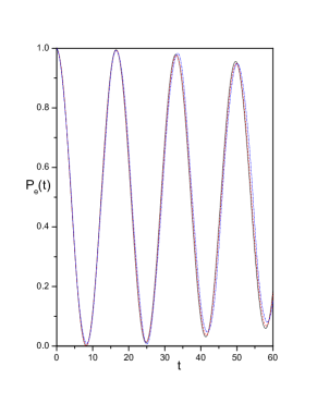
Figure 1: Plot of $P_{e}(t)$ as a function of $t$ for $k=0$, $\nu=1$, $\Omega=0.2$ and $\eta=0.1$. Solid line represents the numerical (exact) solution, dashed line the solution from Section II and the dot-dashed line the solution for the dispersive Hamiltonian of Section III.

$$\hat{H}_{ion}=\nu\hat{n}+\frac{\delta}{2}\hat{\sigma}_{z}+\Omega\left(\hat{\sigma}_{+}\hat{D}(i\eta)+\hat{\sigma}_{-}\hat{D}^{\dagger}(i\eta)\right),$$ (2)

where $\hat{D}(i\alpha)=e^{i\alpha(a+a^{\dagger})}$ is the displacement operator, and $\delta=\omega_{a}-\omega_{L}$ the laser-ion detuning.

II.1 Low intensity regime

The low intensity regime is the well-known regime, where several effects like multi-phonon transitions, Jaynes-Cummings (JC) and anti-JC interactions may be obtained. To solve this regime, we follow first the traditional approach. We start by using Baker-Hausdorff formula Louisel to factor the displacement operators in equation (2) into a product of exponentials and consider $\delta=k\nu$, i.e. an integer multiple of $\nu$ with $k=0,\pm 1,\pm 2,...$, we then obtain

$$\hat{H}_{ion}=\nu\hat{n}+\frac{k\nu}{2}\hat{\sigma}_{z}+\Omega e^{-\eta^{2}/2}\left(\hat{\sigma}_{+}e^{i\eta a^{\dagger}}e^{i\eta a}+\hat{\sigma}_{-}e^{-i\eta a^{\dagger}}e^{-i\eta a}\right).$$ (3)

Now we expand the exponentials of the annihilation and creation operators in Taylor series and get rid off the free Hamiltonians via a transformation to the interaction picture to obtain the Hamiltonian

$$\hat{H}_{I} = \Omega e^{-\eta^{2}/2}$$

$$\times \left(\hat{\sigma}_{-}\sum_{n,m=0}^{\infty}\frac{(-i\eta)^{n+m}}{n!m!}a^{\dagger n}a^{m}e^{i\nu t(n-m+k)}+H.c\right).$$

We use the fact that are in the LIR, $\nu\gg\Omega$ and make the RWA, i.e. we only keep time independent terms in the above Hamiltonian to end up with

$$\hat{H}_{I}=\Omega e^{-\eta^{2}/2}\left(a^{\dagger k}(-i\eta)^{k}\hat{\sigma}_{-}\frac{\hat{n}!}{(\hat{n}+k)!}L_{\hat{n}}^{(k)}(\eta^{2})+H.c\right),$$ (5)

with $L_{\hat{n}}^{(k)}(x)$ the associated Laguerre polynomials of order (operator) $\hat{n}=a^{\dagger}a$. The Hamiltonian above is now readily solvable, so that we may find easily the evolution operator associated to it.

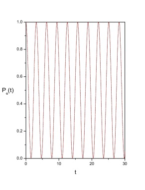
Figure 2: Plot of $P_{e}(t)$ as a function of $t$ for $k=0$, $\Omega=1$, $\nu=0.2$ and $\eta=0.1$. Solid line represents the numerical (exact) solution, dashed line the solution for the dispersive Hamiltonian of Section III .

III Other regimes

Although the atom-field and ion-laser interactions appear to be physically and mathematically quite distinct, they are in fact exactly equivalent. The easiest way to see this is by using the transformation

$$\hat{R}=e^{i\hat{n}\frac{\pi}{2}}e^{\frac{\pi}{4}(\hat{\sigma}_{+}-\hat{\sigma}_{-})}e^{-i\frac{\eta}{2}(\hat{a}+\hat{a}^{\dagger})(\hat{\sigma_{z}})}$$ (6)

such that $\hat{{\mathcal{H}}}_{ion}=\hat{R}\hat{H}_{ion}\hat{R}^{\dagger}$

$$\hat{{\mathcal{H}}}_{ion}=\nu\hat{n}+\Omega\hat{\sigma}_{z}+\frac{\eta\nu}{2}\left(\hat{\sigma}_{+}+\hat{\sigma}_{-}\right)\left(\hat{a}+\hat{a}^{{\dagger}}\right)+\frac{\delta}{2}\left(\hat{\sigma}_{+}+\hat{\sigma}_{-}\right)+\frac{\nu\eta^{2}}{4}.$$ (7)

Therefore we have linearized the ion-laser interaction in an exact way. In the following we will neglect the term $\frac{\nu\eta^{2}}{4}$ because it only represents a constant shift of all the eigenenergies.

III.1 Medium intensity regime (MIR)

We now consider the case where the vibrational frequency is of the order of (twice) the field intensity (Rabi frequency). We also consider the Lamb-Dicke regime, i.e. $\eta\ll 1$. For simplicity we will set $\delta=0$ to show the different possibilities we have now. However it is not difficult to produce effective Hamiltonians also in the off-resonance case. In this case the Hamiltonian (7) may be casted into

$$\hat{{\mathcal{H}}}_{MIR}=\nu\hat{n}+\Omega\hat{\sigma}_{z}+\frac{\eta\nu}{2}\left(\hat{\sigma}_{+}\hat{a}++\hat{a}^{\dagger}\hat{\sigma}_{-}\right)$$ (8)

which is a Hamiltonian that has been extensively studied JCM ; JSM .

III.2 Low and high intensity regimes (HIR)

We have shown in Section II how to solve for the LIR case. Here we will show a different method that is also valid for the HIR.

By transforming the Hamiltonian (7) with the unitary operators

$$\hat{U}_{1}=e^{\xi_{1}(\hat{a}^{\dagger}\hat{\sigma}_{+}-\hat{a}\hat{\sigma}_{-})},\qquad\hat{U}_{2}=e^{\xi_{2}(\hat{a}\hat{\sigma}_{+}-\hat{a}^{\dagger}\hat{\sigma}_{-})},$$ (9)

with $\xi_{1},\xi_{2}\ll 1$, we can remain up to first order in the expansion $e^{\xi A}Be^{-\xi A}=B+\xi[A,B]+\frac{\xi^{2}}{2!}[A,[A,B]]+...\approx B+\xi[A,B]$, so we obtain the effective Hamiltonian

$$\hat{{\mathcal{H}}}_{eff} = \nu\hat{a}^{\dagger}\hat{a}+\Omega\hat{\sigma}_{z}-\chi_{ion}\hat{\sigma}_{z}(\hat{a}^{\dagger}\hat{a}+\frac{1}{2})+\frac{\delta}{2}(\sigma_{+}+\sigma_{-})$$ (10)

$$+ \frac{\kappa}{2}\hat{\sigma}_{z}\left(\hat{a}^{\dagger}+\hat{a}\right).$$

We have used

$$\xi_{1}=\frac{\eta\nu}{2(\nu+2\Omega)}\qquad\xi_{2}=\frac{\eta\nu}{2(2\Omega-\nu)}.$$ (11)

We can see that in fact $\xi_{1},\xi_{2}\ll 1$ either in the LIR (in this case we have also to consider $\eta\ll 1$) or in the HIR (no constrain for $\eta$), which justifies completely the approximation for the above Hamiltonian. For the resonant case, $k=0$, it becomes diagonal and we can solve it in an easy way. In Fig. 1 we show a plot for the probability to find the ion in its excited state. The three curves in the figure correspond to the exact case (solid line), the solution form Hamiltonian (5) (dashed line) and the solution for the dispersive Hamiltonian (10). We can see excellent agreement among the three plots for the LIR. Now, for the HIR we show a plot in Fig. 2 for the numerical solution (solid line) and our solution from this Section (dashed line). Again it may be noticed an excellent agreement between both curves. We should stress that there is no other analytical solution to compare with, as ours is the first analytical solution in this regime (also in the medium regime).

The new interaction constants in the effective Hamiltonian (10) have the form

$$\chi_{ion}=\frac{2\eta^{2}\nu^{2}\Omega}{4\Omega^{2}-\nu^{2}},\quad\kappa=\frac{\delta\eta\nu^{2}}{4\Omega^{2}-\nu^{2}}.$$ (12)

In the resonant case and high intensity regime, $\Omega\gg\nu$, it is easy to show that

$$\chi_{ion}\rightarrow\chi^{high}=\frac{2\eta^{2}\nu^{2}}{4\Omega}\frac{1}{1-\frac{\nu^{2}}{4\Omega^{2}}}\approx\frac{\eta^{2}\nu^{2}}{2\Omega}.$$ (13)

while in the low intensity regime, $\Omega\ll\nu$, we will have the same Hamiltonian but $\chi$ will change to

$$\chi_{ion}\rightarrow\chi_{low}=-2\eta^{2}\Omega\frac{1}{1-\frac{4\Omega^{2}}{\nu^{2}}}\approx-2\eta^{2}\Omega$$ (14)

If in Eq. (10) we take the detuning $\delta$ different from zero, we could get the usual blue and red side-bands interactions (see for instance Ref. tomb ). This is done by choosing the value $\delta=\pm\nu$. The only case in which we can obtain such regimes is the low intensity case, where one can perform the RWA to the Hamiltonian (10), which agrees with the usual procedure for obtaining such blue and red side-band regimes. The high intensity case, $\Omega\gg\nu$ does not allow such side-bands because in the Hamiltonian (10) the interaction constants multiplying the different terms may be of the same order.

IV Conclusions

We have shown that it is possible to solve analytically the ion-laser Hamiltonian in different intensity regimes, from low to high. For the MIR we have casted the ion laser Hamiltonian into a JCM Hamiltonian (for the on-resonant case) that allows easy solution. For the HIR we have found a dispersive Hamiltonian, which, being diagonal, it is direct to solve. We have found excellent agreement between the exact (numerical) solutions and our proposed solutions.

We would like to thank CONACYT for support.

References

- (1) D.J. Wineland, J.J. Bollinger, W.M. Itano, F.L. Moore, and D.J. Heinzen, Phys. Rev. A 46 R6797 (1992).
- (2) D. Leibfried, R. Blatt, C. Monroe y D. Wineland, Rev. of Mod. Phys. 75 281 (2003).
- (3) J. Wineland et al., J. Res. Natl. Inst. Stand. Technol. 103 259 (1998).
- (4) D. Leibfried, D.M. Meekhof, B.E. King, C. Monroe, W.M. Itano, and D.J. Wineland, Phys. Rev. Lett. 77, 4281 (1996).
- (5) S. Wallentowitz and W. Vogel, Phys. Rev. A 59, 531 (1999).
- (6) M. Sasura and V. Buzek, J. of Mod. Optics 49, 1593 (2002).
- (7) H. Moya-Cessa and P. Tombesi, Phys. Rev. A61, 025401 (2000).
- (8) H. Moya-Cessa, D. Jonathan and P.L. Knight, J. of Mod. Optics 50, 265 (2003).
- (9) W.P. Schleich, ”Quantum Optics in Phase Space”, (Wiley-VCH, 2001).
- (10) M. Fernández-Guasti, and H. Moya-Cessa, J. of Phys. A36, 2069 (2003); H. Moya-Cessa and M.F. Guasti, Phys. Lett. A311 1 (2003).
- (11) J.M. Vargas-Martinez and H. Moya-Cessa, J. of Opt. B 6, S618 (2004).
- (12) We can perform the optical rotating wave approximation as the laser and atomic transition frequencies are much, much larger than the field intensity in experiments ion .
- (13) E.T. Jaynes and F.W. Cummings, Proc. IEEE 51, 89 (1963).
- (14) B. W. Shore, and P. L. Knight, J. Mod. Opt. 40, 1195 (1993).
- (15) W.H. Louisell, Quantum Statistical Properties of Radiation, (Wiley, NewYork, 1973).