Who Pulled the Trigger: a Supernova or an AGB Star?

Abstract

The short-lived radioisotope ⁶⁰Fe requires production in a core collapse supernova or AGB star immediately before its incorporation into the earliest solar system solids. Shock waves from a somewhat distant supernova, or a relatively nearby AGB star, have the right speeds to simultaneously trigger the collapse of a dense molecular cloud core and to inject shock wave material into the resulting protostar. A new set of FLASH2.5 adaptive mesh refinement hydrodynamical models shows that the injection efficiency depends sensitively on the assumed shock thickness and density. Supernova shock waves appear to be thin enough to inject the amount of shock wave material necessary to match the short-lived radioisotope abundances measured for primitive meteorites. Planetary nebula shock waves from AGB stars, however, appear to be too thick to achieve the required injection efficiencies. These models imply that a supernova pulled the trigger that led to the formation of our solar system.

1 Introduction

Primitive meteorites contain daughter products of the decay of short-lived radioisotopes (SLRIs) such as ²⁶Al, ⁴¹Ca, ⁵³Mn, and ⁶⁰Fe, distributed in different minerals in a way that indicates the parent isotopes were still alive at the time of their incorporation into the refractory inclusions and chondrules that record the earliest history of the solar system. The presence of ⁶⁰Fe is particularly significant, as its production requires stellar nucleosynthesis (Tachibana & Huss 2003; Tachibana et al. 2006). Given half-lives on the order of $\sim 10^{6}$ yr, the evidence for these radioisotopes suggests that the same stellar source that synthesized them may well have triggered the collapse of the presolar dense cloud core as well, while simultaneously injecting the freshly-synthesized radioisotopes (Cameron & Truran 1977; Boss 1995). Supernovae resulting from massive stars in the range of $\sim 20M_{\odot}$ to $\sim 60M_{\odot}$ or planetary nebulae derived from intermediate-mass ($\sim 5M_{\odot}$) AGB stars have been proposed as possible sources of all or most of these radioisotopes (e.g., Huss et al. 2009).

Shock-triggered collapse and injection into the presolar cloud (Cameron & Truran 1977) has been proposed and studied in detail (e.g., Boss 1995; Foster & Boss 1997; Vanhala & Boss 2002; Boss et al. 2008, 2010). Recent calculations have shown that simultaneous triggered gravitational collapse and injection of shock wave gas and dust into the collapsing cloud core is possible even when detailed heating and cooling processes in the shock-cloud interaction are included (Boss et al. 2008). Shock speeds in the range from 5 km/sec to 70 km/sec are capable of achieving simultaneous triggering and injection for a 2.2 $M_{\odot}$ target cloud (Boss et al. 2010). However, these models led to considerably lower injection efficiencies than those previously estimated on the basis of models where the shock-cloud interaction was assumed to be isothermal (Boss 1995; Foster & Boss 1997; Vanhala & Boss 2002). When the injection efficiency ($f_{i}$) is defined to be the fraction of the incident shock wave material that is injected into the collapsing cloud core, values of $f_{i}\sim 0.001$ result from the nonisothermal models (Boss et al. 2008, 2010), about 100 times lower than the values of $f_{i}$ found previously for strictly isothermal interactions. Considering that the shock fronts in these models contain 0.015 $M_{\odot}$ of gas and dust, this means that the Boss et al. (2008, 2010) models produced nominal dilution factors $D\sim 10^{-5}$, where $D$ is defined as the ratio of the amount of mass derived from the stellar source of the shock front that ends up in the protoplanetary disk to the amount of mass in the disk that did not derive from the stellar source. Such values appear to be much too low to explain the initial abundances inferred for typical SLRIs, which range from $\sim 10^{-4}$ to $\sim 3\times 10^{-3}$ for supernovae (Takigawa et al. 2008; Gaidos et al. 2009) and $\sim 3\times 10^{-3}$ for an AGB star (Trigo-Rodríguez et al. 2009).

Boss et al. (2010) found that varying the shock speed from 5 to 70 km/sec had relatively little effect on $f_{i}$, while doubling the density of the target cloud could decrease $f_{i}$ by a factor of 3. Here we explore the effects of changes in the assumed shock wave parameters, in order to learn if higher values of $f_{i}$ and therefore $D$ might thereby result. In addition, we seek to learn if these shock wave variations will indicate a preference for either a supernova or an AGB star wind for triggering the formation of the solar system.

2 Numerical Methods

We used the FLASH2.5 code, as in our previous work (Boss et al. 2008, 2010). FLASH2.5 advects gas using the piecewise parabolic method, accurate to second-order in space and time, with a Riemann solver at cell boundaries designed to handle strong shock fronts. Our tests of the FLASH2.5 code and further details about our implementation scheme are detailed in Boss et al. (2010). Basically, we used the two dimensional, cylindrical coordinate ($R,Z$) version of FLASH2.5, with axisymmetry about the rotational axis ($\hat{z}$). Multipole self-gravity was used, including Legendre polynomials up to $l=10$. The cylindrical grid was typically 0.2 pc long in $Z$ and 0.063 pc wide in $R$, though in some models the grid was extended to be 0.4 pc long in order to follow the evolution farther downstream. The number of blocks in $R$ ($N_{BR}$) was 5 in all cases, while the number of blocks in $Z$ ($N_{BZ}$) was 15 for the standard-length grids and 20 for the extended grids, with each block consisting of $8\times 8$ grid points. The number of levels of grid refinement ($N_{L}$) was 5 for all models.

As in Boss et al. (2008, 2010), we included compressional heating and radiative cooling, based on the results of Neufeld & Kaufman (1993) for cooling caused by rotational and vibrational transitions of optically thin, warm molecular gas composed of H₂O, CO, and H₂. As before, we assumed a radiative cooling rate of $\Lambda\approx 9\times 10^{19}(T/100)\rho^{2}$ erg cm^-3 s^-1, where $T$ is the gas temperature in K and $\rho$ is the gas density in g cm^-3. The gas temperatures were constrained to lie in the range between 10 K and 1000 K, as in Boss et al. (2008, 2010), based on the results of Kaufman & Neufeld (1996) for magnetic shock speeds in the desired range of 5 km/sec to 45 km/sec.

3 Initial Conditions

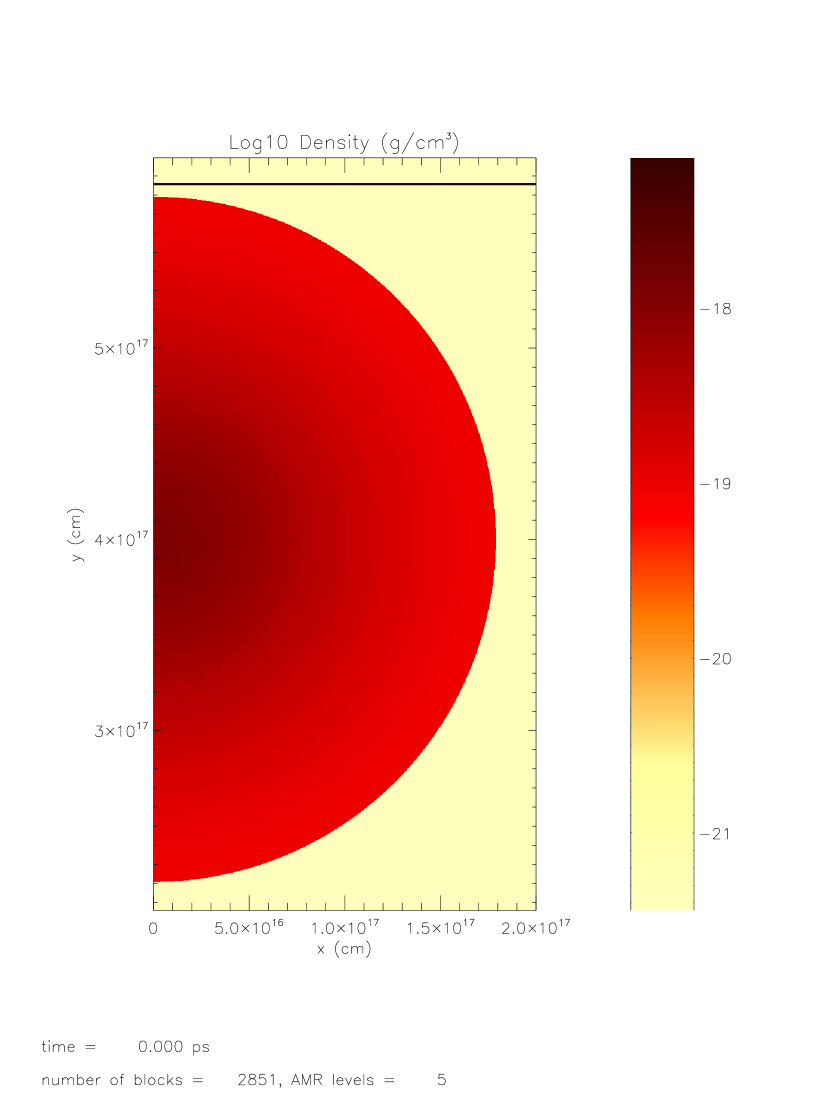
Figure 1: Initial log density distibution for model 200-0.1. Black contours (top) enclose shock front material (representing SLRI), which is moving downward and is about to strike the target cloud. The shock front has a thickness of 0.003 pc and a density of $3.6\times 10^{-20}$ g cm^-3. Left side is the symmetry axis, with $R$ horizontal and $Z$ vertical.

The target dense cloud cores are modeled on Bonner-Ebert (BE) spheres (Bonnor 1956), which are the equilibrium structures for self-gravitating, isothermal spheres of gas. As in Boss et al. (2010), the BE-like spheres are initially isothermal at 10 K, with a central density of $1.24\times 10^{-18}$ g cm^-3, a radius of 0.058 pc, a mass of 2.2 $M_{\odot}$, and are stable against collapse for at least $10^{6}$ yr. The spheres are embedded in an intercloud medium with a density of $3.6\times 10^{-22}$ g cm^-3 and a temperature of 10 K. Shock waves are launched downward from the top of the grid toward the spheres (Figure 1) at a speed of 40 km/sec. The standard shock front, as used in Boss et al. (2008, 2010), has a thickness of 0.003 pc with a uniform density of $3.6\times 10^{-20}$ g cm^-3, a mass of 0.015 $M_{\odot}$, a temperature of 1000 K, and is followed by a post-shock wind with a density of $3.6\times 10^{-22}$ g cm^-3 and temperature of 1000 K, also moving downward at the same speed as the shock wave. The shock front material is represented by a color field, initially defined to be equal to 1 inside the shock front and 0 elsewhere, which allows the shock wave material to be tracked forward in time (e.g., Foster & Boss 1997).

4 Results

Table 1 lists the variations in the shock front parameters that were explored in the new models as well as the resulting injection efficiencies $f_{i}$ and dilution factors $D$. The models are all identical except for the assumed properties of the initial shock front, where the standard shock front densities of Boss et al. (2010) were multiplied by factors ranging from 0.1 to 800, and the shock thickness by factors ranging from 0.1 to 10.

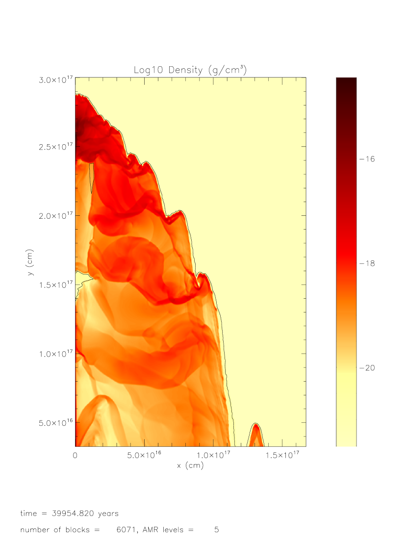
Figure 2: Cloud density after 0.04 Myr, plotted in the same manner as in Figure 1. Instabilities at the shock-cloud interface have injected shock wave material throughout most of the target cloud while ablating the outer regions into the downstream flow.

Figure 1 shows the initial conditions for model 200-0.1, where the initial shock density was 200 times the standard value and the initial shock thickness was 0.1 times the standard value. Figure 2 shows the shock-cloud interaction 0.04 Myr after Figure 1, when the shock front has begun to drive the target cloud into collapse: the maximum density has increased by nearly a factor of 1000. Rayleigh-Taylor fingers have injected shock-front material throughout most of the target cloud (as shown by the black contours outlining the color field, initially in the shock front), while Kelvin-Helmholtz instabilities are ablating the outer regions of the cloud and transporting it downstream.

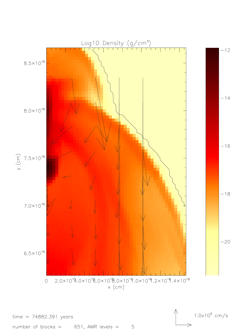
Figure 3: Inner collapsing region of the cloud after 0.075 Myr, plotted as before, showing the dense gas along the symmetry axis. Velocity vectors are plotted for every eighth AMR grid point.

Figure 3 shows the 1000-AU-scale region around the dense, collapsing protostar whose collapse has been triggered by the shock front. The velocity vectors show that while more gas will be accreted by the protostar, other gas is likely to be blown downstream by the combination of the shock front and the post-shock wind and will not be accreted. The mass of the protostar at this time is $\sim 1M_{\odot}$, implying that roughly half of the target cloud’s initial mass will be lost and half accreted by the protostar. Figure 4 depicts the color field at the same time and on the same spatial scale as Figure 3, showing that shock front material has already been injected into the collapsing protostar, and that more shock front material will be accreted as the collapse proceeds. The bulk of the shock front material is swept downstream, however.

The injection efficiency estimated for model 200-0.1 at the time shown in Figures 3 and 4 is $f_{i}\approx 0.02$, while the dilution factor for this model is $D\approx 3\times 10^{-3}$. Most of the models shown in Table 1 behaved in much the same way as model 200-0.1, with the exception of the models marked by asterisks. In these models, the shock front was so vigorous that while the target cloud was compressed somewhat, the cloud did not reach a high enough density for dynamic, self-gravitational collapse to begin, and by the time that the cloud was pushed off the bottom of the numerical grid, the shock had shredded the cloud more than it had triggered collapse. Hence, these models must be considered as failed models, in spite of their high values of $f_{i}$ and $D$: evidently the threat of shredding limits the injection efficiency. Table 1 shows the important trends that for a fixed shock density, increasing the shock thickness results in higher dilution factors $D$, as does increasing the shock density at fixed shock thickness, as might be expected, with cloud shredding placing the ultimate limits on these trends.

Given that $f_{i}\approx 0.02$ and $D\approx 3\times 10^{-3}$ for model 200-0.1, values that are factors of $\sim 20$ and $\sim$ 100 times higher than in the standard shock front model (Boss 2010), respectively, it is clear that injection efficiencies and dilution factors depend sensitively on the assumed shock wave parameters, all other things being equal.

5 Discussion

We now turn to the question of whether any of the injection efficiencies and dilution factors shown in Table 1 are able to match the demands of the meteoritical record for the SLRIs, and in particular, whether any such desirable shock waves might exist in reality.

5.1 Supernova

The desired dilution factors for a supernova trigger range from $D=1.3\times 10^{-4}$ to $1.9\times 10^{-3}$ (Takigawa et al. 2008) to $D=3\times 10^{-3}$ (Gaidos et al. 2009). Table 1 shows that four collapse models had $D$ values in this broad range: models 100-0.1, 200-0.1, 400-0.1, and 10-1. However, these are not the appropriate $D$ values for comparison with a supernova source, because a supernova shock launched at $\sim$ 1000 km/sec must snowplow $\sim$ 25 times its own mass in order to slow down to $\sim$ 40 km/sec (Boss et al. 2010). The model dilution factors in Table 1 must then be decreased by this same factor, dropping $D$ to $\sim 1.2\times 10^{-4}$ for model 200-0.1 and $\sim 4\times 10^{-4}$ for model 400-0.1. These values are close to those proposed by Takigawa et al. (2008), but about 10 times smaller than that favored by Gaidos et al. (2009). As noted by Boss et al. (2010), other factors can result in higher values of $D$ for the models, such as incomplete accretion of the target cloud (e.g., Figure 4, which would raise $D$ for model 200-0.1 by a factor of 2), preferential addition of the late arriving SLRIs to the solar nebula, rather than the protosun, and lower target cloud densities (and consequently larger initial cloud diameters). Given that all of these factors work in the direction of increasing $D$, the fact that both models 200-0.1 and 400-0.1 produce $D$ estimates much closer to the desired range than the standard shock models (Boss et al. 2010) must be viewed as a positive outcome for a supernova trigger.

However, a successful outcome demands that supernova shock waves in their radiative phase have properties similar to those of the shocks assumed in models 200-0.1 and 400-0.1, where the shock thickness was $10^{15}$ cm and the shock number densities were $2\times 10^{6}$ cm^-3 and $4\times 10^{6}$ cm^-3, respectively. The Cygnus Loop, the $\sim 10^{4}$-yr-old remnant of a core collapse (Type II) supernova, has a shock speed of 170 km/sec and a thickness no greater than $\sim 10^{15}$ cm (Blair et al. 1999), consistent with models 200-0.1 and 400-0.1. W44 is a $\sim 2\times 10^{4}$-yr-old remnant of a Type II supernova, where the shock fronts are colliding with giant molecular cloud (GMC) gas with a density greater than $10^{3}$ cm^-3 (Reach, Rho, & Jarrett 2005). The shock front has slowed down to 20-70 km/sec and has thickened as a result of the GMC interaction, but is no thicker than $\sim 10^{17}$ cm. For a nearly isothermal shock, the post-shock density $n_{s}$ for propagation in a stationary medium of density $n_{m}$ is $n_{s}/n_{m}=(v_{s}/c_{m})^{2}$, where $v_{s}$ is the shock speed and $c_{m}$ is the sound speed in the medium (e.g., Spitzer 1968). For the present models, $v_{s}=40$ km/sec, $c_{m}=0.2$ km/sec, and $n_{m}=10^{2}$ cm^-3, leading to $n_{s}=4\times 10^{6}$ cm^-3. This is the same shock density as used in model 400-0.1. Evidently, then, models 200-0.1 and 400-0.1 do appear to be reasonable models of evolved Type II supernova remnants similar to the Cygnus Loop and W44, which have expanded to sizes of 10 pc or more after $\sim 10^{4}$ yr of evolution.

5.2 AGB star wind

Trigo-Rodríguez et al. (2009) suggest that $D\sim 3\times 10^{-3}$ is required for an AGB star source of the SLRIs. Only models 200-0.1 and 400-0.1 produced $D$ values at least this large. Note that dilution caused by snowplowing does not need to be invoked here because planetary nebulae speeds are already in the proper range of 20 to 30 km/sec. However, the thickness of the planetary nebula Abell 39 is estimated to be $\sim 3\times 10^{17}$ cm (Jacoby, Ferland, & Korista 2001) and for planetary nebula PFP-1 to be $\sim 5\times 10^{17}$ cm (Pierce et al. 2004). These thicknesses are even greater than those in the models with 10 times the standard shock thickness (Table 1), and so are incapable of producing the desired dilution factor. Planetary nebulae appear to be too thick to achieve the injection efficiencies needed to explain the solar system’s SLRIs.

5.3 Grain injection

The $D$ values in Table 1 are based on injection purely in the gas phase, i.e., assuming that the SLRIs are either in the gas phase or are locked up in grains small enough to remain tied to the gas. As noted by Foster & Boss (1997), large dust grains can shoot through the gas of a stalled shock front as a result of their momentum, thereby increasing the SLRI injection efficiency, as studied by Ouellette et al. (2010). Hence the $D$ values in Table 1 should be considered as lower bounds.

The penetration distance of a dust grain with a radius $a_{d}$ and density $\rho_{d}$ moving in a gas of density $\rho_{g}$ can be estimated by the distance it must travel to impact an amount of gas equal to its own mass, thereby halving its speed. This distance is $d=4/3(\rho_{d}/\rho_{g})a$. The region at the top of Figure 4 shows that dust grains might be preferentially injected if they could penetrate a distance of $d\sim 10^{16}$ cm into gas with a density $\rho_{g}\sim 10^{-18}$ g cm^-3. With $\rho_{d}=2.5$ g cm^-3, this requires grains with a size $a\sim 30$ $\mu$m or larger.

The predicted power-law size distribution for dust grains formed by core collapse supernovae (e.g., Nozawa et al. 2003) places most of the mass of the grains in the size range from 0.1 $\mu$m to 0.3 $\mu$m (Nath, Laskar, & Shull 2008). Presolar SiC grains of type ”X” that originate in supernovae have sizes that fall in the range of 0.4 $\mu$m to 2 $\mu$m (Amari et al. 1994; Ouellette et al. 2010), with most of the mass being in 0.4 $\mu$m grains. However, Bianchi & Schneider (2007) predict that amorphous carbon grains formed in supernova ejecta have grain sizes less than 0.1 $\mu$m and that oxide grains are smaller than 0.01 $\mu$m. All of these estimates are considerably smaller than 30 $\mu$m: apparently most supernova grains are too small to raise the injection efficiencies significantly.

Bernatowicz, Croat & Daulton (2006) find that most presolar SiC grains formed around carbon AGB stars fall in the size range of 0.1 to 1 $\mu$m, with some as large as 6 $\mu$m (Amari et al. 1994). The carrier grains of SLRIs such as ²⁶Al, ⁴¹Ca, ⁵³Mn, and ⁶⁰Fe are likely to be oxide grains though, not SiC, and only a relatively few oxide grains have been found to date. Current analytical techniques preclude the isotopic identification of presolar grains much smaller than $\sim$ 0.1 $\mu$m. While it thus appears that AGB stars produce somewhat larger grains than supernova remnants, even these grains do not appear to be large enough to raise the injection efficiencies by a significant factor. Hence we conclude that injection efficiencies calculated purely on the basis of gas-phase injection (Table 1), while lower bounds, appear to be close enough to the correct results to rule out AGB stars as the source of the solar system’s SLRIs.

6 Conclusions

A new set of models with varied shock densities and thicknesses has shown that injection efficiencies $f_{i}$ and dilution factors $D$ can be increased by large factors ($>$ 10 and $>$ 1000, respectively), large enough to maintain the viability of this SLRI injection mechanism. Observations of supernova remnants and planetary nebulae imply that while the former shock fronts are thin enough to be suitable for SLRI injection, the latter are not. These results lend support to previous studies that have favored a supernova over an AGB star for the source of the solar system’s SLRIs. Huss et al. (2009) found that an intermediate-mass AGB star could explain the production of ²⁶Al, ⁴¹Ca, ⁶⁰Fe, but not that of ⁵³Mn. Kastner & Myers (1994) pointed out that AGB stars are seldom found in the vicinity of star-forming regions, so the chances of SLRI injection from a planetary nebula wind into a dense cloud core are small. The culprit appears to have been a long-forgotten supernova remnant that swept through the galaxy $\sim$ 4.56 Gyr ago.

Table 1: Injection efficiencies $f_{i}$ (top three rows) and dilution factors $D$ (bottom three rows) as a function of shock density and thickness factors compared to the standard values of $3.6\times 10^{-20}$ g cm^-3 and 0.003 pc, respectively. For a supernova shock front slowed by snowplowing, the $D$ values will be further reduced. Asterisks denote clouds that did not collapse.

shock density $\times$		0.1	1	10	100	200	400	800
thickness $\times$ 0.1	$f_{i}=$	–	2E-4	2E-3	1E-2	2E-2	4E-2	6E-2*
thickness $\times$ 1	$f_{i}=$	6E-5	1E-3	3E-3	1E-2*	–	–	–
thickness $\times$ 10	$f_{i}=$	–	4E-4	2E-3*	–	–	–	–
thickness $\times$ 0.1	$D=$	–	1E-8	1E-6	7E-4	3E-3	1E-2	3E-2*
thickness $\times$ 1	$D=$	4E-8	7E-6	2E-4	7E-3*	–	–	–
thickness $\times$ 10	$D=$	–	3E-5	1E-3*	–	–	–	–

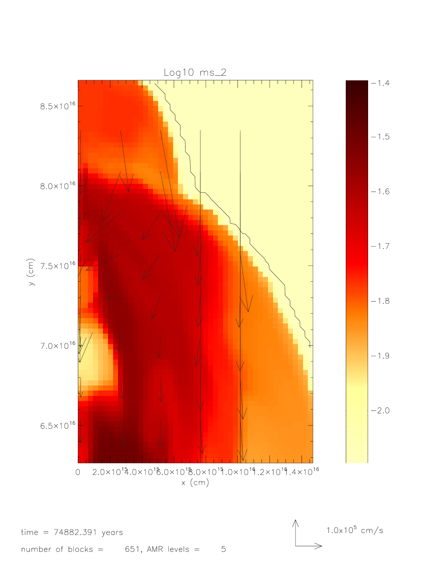
Figure 4: Log shock color density (SLRIs) distribution after 0.075 Myr, showing the same region as in Figure 3. SLRIs have been injected inside the growing protostar and more are infalling onto it.

References

- (1)
- (2) Amari, S., Lewis, R. S., & Anders, E. 1994, Geochim. Cosmochim. Acta, 58, 459
- (3)
- (4) Bernatowicz, T. J., Croat, T. K., & Daulton, T. L. 2006, in Meteorites and the Early Solar System II, ed. D. S. Lauretta & H. Y. McSween (Tucson, AZ: Univ. Arizona Press), 109
- (5)
- (6) Bianchi, S., & Schneider, R. 2007, MNRAS, 378, 973
- (7)
- (8) Blair, W. P., Sankrit, R., Raymond, J. C., & Long, K. S. 1999, AJ, 118, 942
- (9)
- (10) Bonnor, W. B. 1956, MNRAS, 116, 351
- (11)
- (12) Boss, A. P. 1995, ApJ, 439, 224
- (13)
- (14) Boss, A. P., et al. 2008, ApJ, 686, L119
- (15)
- (16) ——. 2010, ApJ, 708, 1268
- (17)
- (18) Cameron, A. G. W., & Truran, J. W. 1977, Icarus, 30, 447
- (19)
- (20) Chevalier, R. 1974, ApJ, 188, 501
- (21)
- (22) Foster, P. N., & Boss, A. P. 1996, ApJ, 468, 784
- (23)
- (24) ——. 1997, ApJ, 489, 346
- (25)
- (26) Frank, A., & Mellema, G. 1994, A&A, 289, 937
- (27)
- (28) Gaidos, E., Krot, A. N., Williams, J. P., & Raymond, S. N. 2009, ApJ, 696, 1854
- (29)
- (30) Huss, G. R., et al. 2009, Geochim. Cosmochim. Acta, 73, 4922
- (31)
- (32) Jacoby, G. H., Ferland, G. J., & Korista, K. T. 2001, ApJ, 560, 272
- (33)
- (34) Kastner, J. H., & Myers, P. C. 1994, ApJ, 421, 605
- (35)
- (36) Kaufman, M. J., & Neufeld, D. A. 1996, ApJ, 456, 611
- (37)
- (38) Nath, B. B., Laskar, T., & Shull, J. M. 2008, ApJ, 682, 1055
- (39)
- (40) Neufeld, D. A., & Kaufman, M. J. 1993, ApJ, 418, 263
- (41)
- (42) Nozawa, T., et al. 2003, ApJ, 598, 785
- (43)
- (44) Ouellette, N., Desch, S. J., & Hester, J. J. 2010, ApJ, 711, 597
- (45)
- (46) Pierce, M. J., Frew, D. J., Parker, Q. A., & Köppen, J. 2004, Publ. Astron. Soc. Australia, 21, 334
- (47)
- (48) Plait, P., & Soker, N. 1990, AJ, 99, 1883
- (49)
- (50) Reach, W. T., Rho, J., & Jarrett, T. H. 2005, ApJ, 618, 297
- (51)
- (52) Spitzer, L. 1968, Difuse Matter in Space (New York, NY: J. Wiley & Sons), 168
- (53)
- (54) Tachibana, S., & Huss, G. R. 2003, ApJ, 588, L41
- (55)
- (56) Tachibana, S., et al. 2006, ApJ, 639, L87
- (57)
- (58) Takigawa, A., et al. 2008, ApJ, 688, 1382
- (59)
- (60) Trigo-Rodríguez, J. M., et al. 2009, Meteorit. & Planet. Sci., 44, 627
- (61)
- (62) Vanhala, H. A. T., & Boss, A. P. 2002, ApJ, 575, 1144
- (63)